Analysis of Factors Influencing Energy Efficiency Based on Spatial Quantile Autoregression: Evidence from the Panel Data in China

Abstract

This research mainly studies the factors influencing the efficiency of energy utilization. Firstly, by calculating $Mora{n}^{’}sI$ and local indicators of spatial association (LISA) of energy efficiency of regions in mainland China, we found that energy efficiency shows obvious spatial autocorrelation and spatial clustering phenomena. Secondly, we established the spatial quantile autoregression (SQAR) model, in which the energy efficiency is the response variable with seven influence factors. The seven factors include industrial structure, resource endowment, level of economic development etc. Based on the provincial panel data (1998–2016) of mainland China (data source: China Statistical Yearbook, Statistical Yearbook of provinces), the findings indicate that level of economic development and industrial structure have a significant role in promoting energy efficient. Resource endowment, government intervention and energy efficiency show a negative correlation. However, the negative effect of government intervention is weakened with the increase of energy efficiency. Lastly, we compare the results of SQAR with that of ordinary spatial autoregression (SAR). The empirical result shows that the SQAR model is superior to SAR model in influencing factors analysis of energy efficiency.

1. Introduction

With the rapid development of the global economy, energy demand and consumption are increasing extensively, which has also brought some problems, such as environmental pollution, global warming, excessive exploitation of resources etc. For sustainable economic development and social progress, it is very important to improve energy efficiency and formulate relevant policies. There are some studies focused on how to put the energy system onto a more sustainable path from a macro perspective. See for example [1,2,3,4,5] and references therein.

The reasonable calculation method of energy utilization efficiency and quantitative analysis of influence factors are necessary and important for policymakers. Tobler, an American geographer in [6] proposed that everything is related to everything else, but near things are more related to each other, which is also known as Tobler’s First Law of Geography. The energy efficiency of one region also can be influenced by neighboring regions. Some studies showed the spatial auto-correlation and clustering phenomenon of energy efficiency. For example, Shen and Liu [7] used the data envelopment analysis (DEA) model to measure the energy efficiency values of 30 provinces in China from 1992 to 2007. The result shows that there are obvious spatial aggregation phenomena in provincial energy efficiency.

Concerning research on influence factors of energy efficiency, there are some literatures, for example [7,8,9,10,11,12,13,14,15] etc. Shen and Liu [7] studied influence factors by using SAR and threshold regression models. Liu and Mao [10] studied the factors influencing energy efficiency by using a spatial lagged model (SLM, also called SAR in literature) and spatial error model (SEM) based on the data of 29 provinces and cities in China from 2000 to 2012. They did not consider the test of homoscedasticity of explanatory variables, which is required before building SLM and SEM. Makridou et al. (2016) [8] analyzed the energy efficiency of five energy-intensive industries in 23 European Union countries by using a two-level cross-classified model. Li and Shi (2014) in [9] proposed an improved super-SBM (slacks-based measure) model to analyze the energy efficiency of Chinese industrial sectors. Jiang et el. [12] analyzed energy efficiency of provinces in China by using the ordinary spatial Dubin error model for panel data. Li and Lin (2018) [13] studied the direct and indirect effects of different types of technological progress on China’s energy efficiency.

To the best of our knowledge, existing references about influence factors of energy efficiency used ordinary regression without considering different quantiles. However, the ordinary regression model characterizes the relationship between the expectation of the explained variable and explanatory variables, which is not robust to outliers. To this end, the quantile regression model is a good way to deal with outliers, which can describe more detail of data. Since Koenker and Bassett [16] proposed the quantile regression method in 1978, the quantile idea has been widely used and developed (see e.g., [17,18]).

The purpose of this work is to analyze the factors influencing the efficiency of energy utilization based on the spatial quantile autogression model, so as to provide some advice on how to improve energy efficiency for decision-makers. As far as we know, the SQAR model has not been employed in existing references related to this topic. Why do we use quantiles? Quantile regression is robust to outliers. By considering different quantiles, we can get different coefficients of factors, which can reveal the relationship between factors and energy efficiency more comprehensively. Based on the work [19], we combine spatial autoregression with quantiles to study factors influencing the efficiency of energy. Firstly we analyze the $Mora{n}^{’}sI$ ([20]), local indicators of spatial association (LISA) of provincial energy efficiencies of China. The data set for empirical analysis comes from China Statistical Yearbook, Statistical Yearbook of provinces and http://data.stats.gov.cn, http://www.tjcn.org (1998–2016). The $Mora{n}^{’}sI$ and LISA of energy efficiency show that energy efficiency possesses obvious spatial autocorrelation and spatial aggregation. Secondly, thanks to the spatial dependence of energy efficiency, we use the spatial quantile autoregressive model of panel data to analyze the influence of seven factors on energy efficiency at different quantile levels. The conclusion shows that the industrial structure, economic development level and technical level have a positive effect on the provincial energy efficiency in China. Resource endowment shows a negative correlation to energy efficiency. According to the empirical analysis based on the real data, the SQAR model is superior to the ordinary spatial autoregressive model in analyzing influence factors of energy efficiency.

The rest of the paper is organized as follows: Section 2 is about the methods and models including the measurement of efficiency of energy utilization, $Mora{n}^{’}sI$, LISA and SQAR. In Section 3, we apply the models to the provincial data of China during the years of 1998–2016 to analyze the efficiency of energy utilization.

2. Methods and Models

2.1. Spatial Auto-Correlation Test Based on $Mora{n}^{’}sI$ Index

In this subsection, we introduce the measurement of energy efficiency, $Mora{n}^{’}sI$ and LISA which are employed to test the spatial autocorrelation of energy efficiency.

For the measurement of energy efficiency, we use the data envelopment analysis (DEA) by taking the so-called low-carbon GDP [19] as the output variable. For convenience, we briefly describe the method of data envelopment analysis here. Assume there are n regions or called decision making units (DMU) in some references. Each region has m input variables and k output variables. For a year in the j-th region, $x_j={(x_{1j},x_{2j},\cdots ,x_{mj})}^{\prime }$ and $y_j={(y_{1j},\cdots ,y_{kj})}^{\prime }$$(j=1,2,\cdots ,n)$ represent input and output vectors respectively, whose corresponding weight vectors are denoted by $\mu ={({\mu }_1,\cdots ,{\mu }_m)}^{\prime }$ and $\nu ={({\nu }_1,\cdots ,{\nu }_k)}^{\prime }$ respectively. The CRS-DEA model [21] of the j-th region can be expressed as follows:

$$\underset{\mu ,\nu }{max}({\nu }^{\prime }{y}_j/{\mu }^{\prime }{x}_j)$$

$$s.t\left\{\begin{array}{c}{\nu }^{\prime }{y}_i/{\mu }^{\prime }{x}_i\le 1,,i=1,2,\cdots ,n,\hfill \\ \mu \ge 0,\nu \ge 0.\hfill \end{array}\right.$$

(1)

The dual problem of model (1) can be expressed as:

$$min{\theta }_j$$

$$s.t\left\{\begin{array}{c}\sum _{i=1}^n{x}_{si}{\lambda }_i\le {\theta }_j{x}_{sj},s=1,\cdots ,m\hfill \\ \sum _{i=1}^n{y}_{si}{\lambda }_i\ge y_{sj},s=1,\cdots ,k\hfill \\ {\lambda }_i\ge 0,i=1,2,\cdots ,n,\hfill \end{array}\right.$$

(2)

where ${\theta }_j$$(0<{\theta }_j\le 1)$ is a scalar, the efficiency value of the j-th region. It embodies the region’s ability to effectively allocate resources and sustainable development capability. If ${\theta }_j=1$, it means that the j-th region is located at the production frontier, that is, the j-th region that obtains the maximum output under certain input is effective. $\lambda$ is an $n\times 1$ vector of constants. It serves to form a convex combination of observed inputs and outputs.

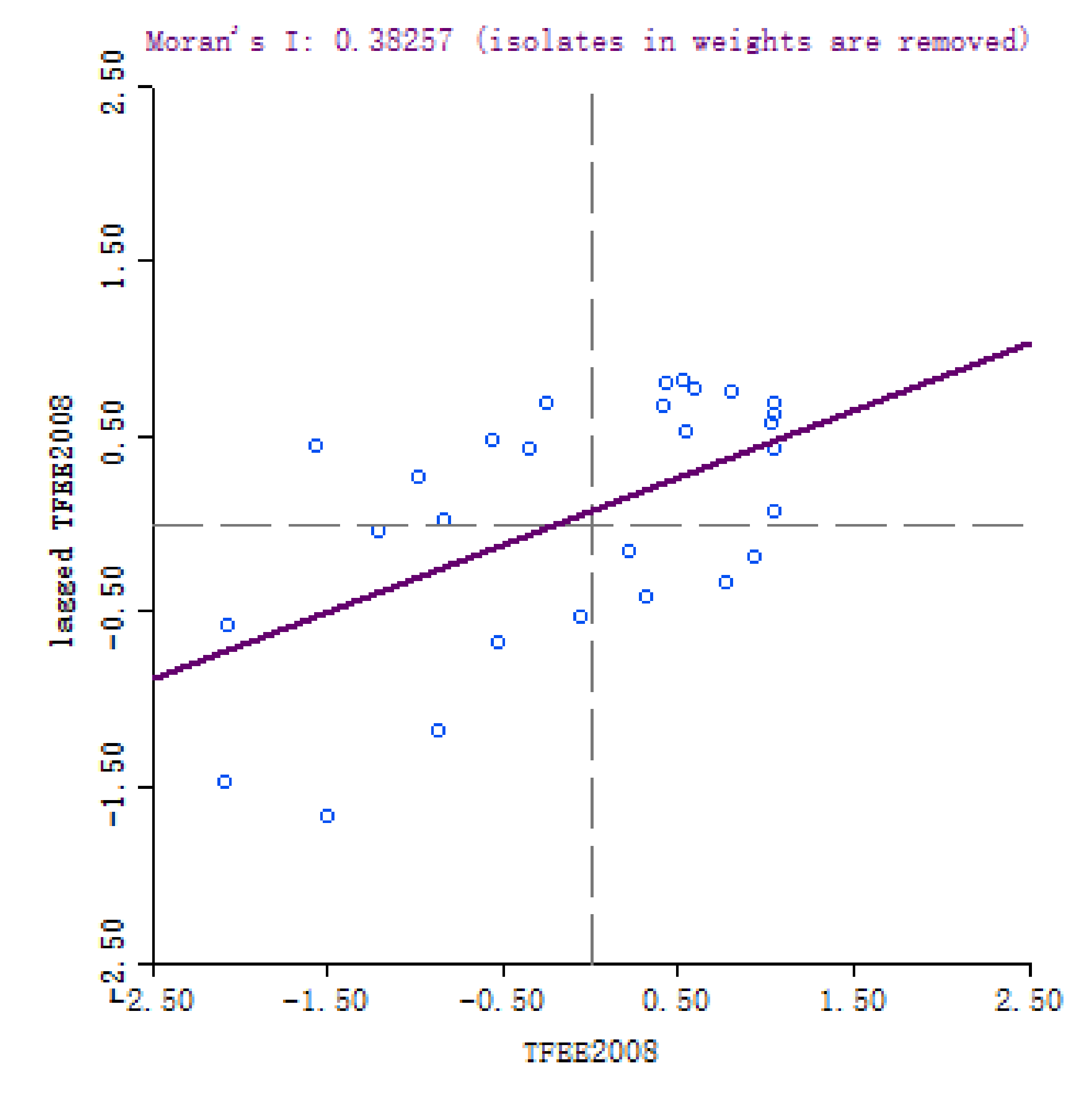
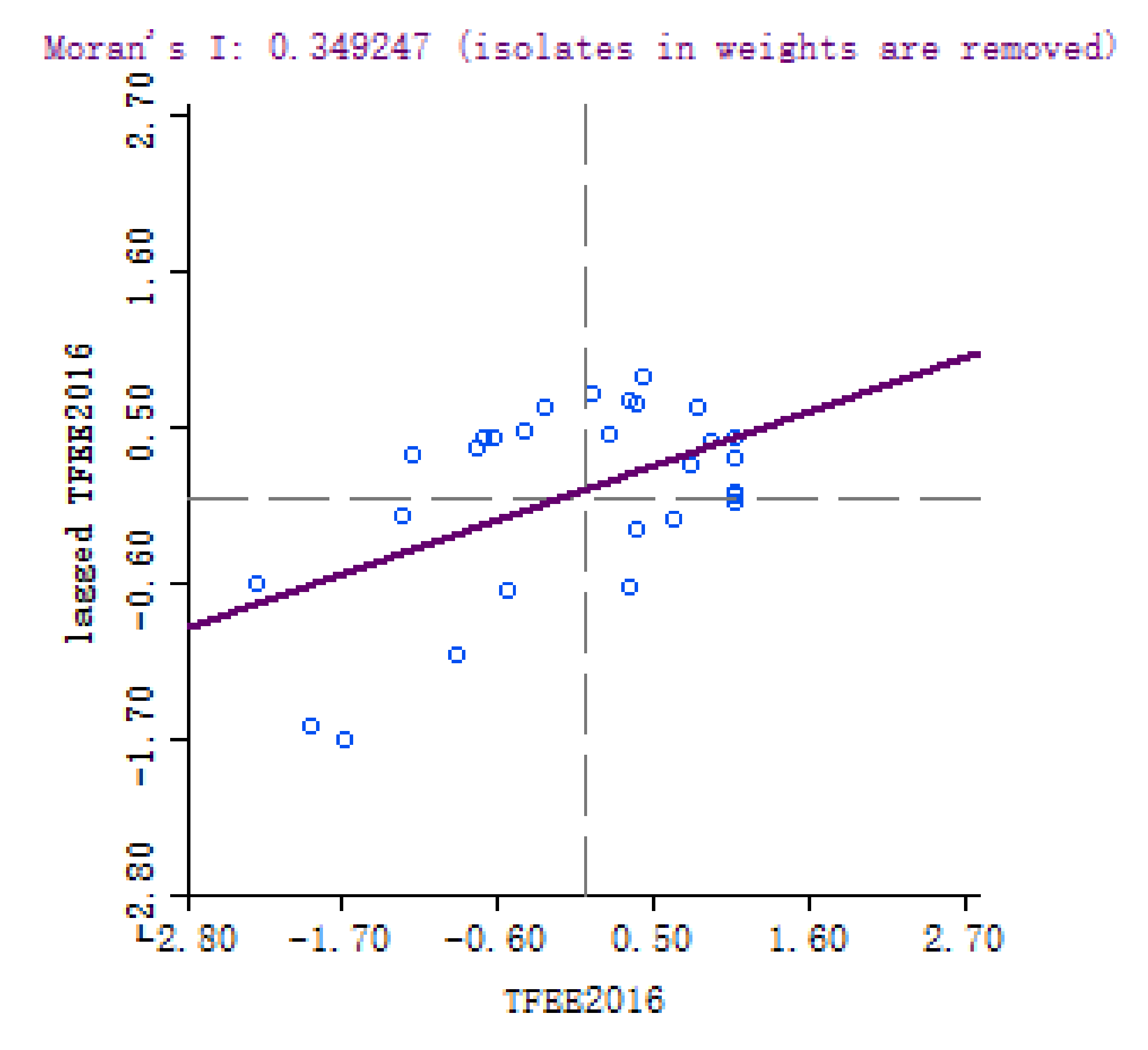
The global $Mora{n}^{’}sI$ describes the global spatial autocorrelation of all data, which is defined as follows [20]:

$$\begin{array}{cc}\hfill I& =\frac{n{\sum }_{i=1}^n{\sum }_{j=1}^n{w}_{ij}(x_i-\overline{x})(x_j-\overline{x})}{{\sum }_{i=1}^n{\sum }_{j=1}^n{w}_{ij}{\sum }_{j=1}^n{(x_j-\overline{x})}^2}\hfill \\ \hfill & =\frac{{\sum }_{i=1}^n{\sum }_{j=1}^n{w}_{ij}(x_i-\overline{x})(x_j-\overline{x})}{S^2{\sum }_{i=1}^n{\sum }_{j=1}^n{w}_{ij}},\hfill \end{array}$$

(3)

where $S^2=\frac{1}{n}{\sum }_{i=1}^n{(x_i-\overline{x})}^2$, n the number of areas (spatial units), $x_i$ the energy efficiency value of the i-th region, $w_{ij}$ the element of the spatial weight matrix, which represents the adjacent relationship between the i-th region and the j-th region. It is defined as follows:

$$w_{ij}=\left\{\begin{array}{c}1Ifareaiisadjacenttoareaj\hfill \\ 0Ifareaiisnotadjacenttoareaj.\hfill \end{array}\right.$$

(4)

The design of the spatial weight matrix in this paper follows the rook adjacency method. That is, if there is a common boundary between the two regions, they are considered to be adjacent. Using this method, a spatial weight matrix can be constructed.

The range of $Mora{n}^{’}sI$ is $[-1,1]$. A positive $Mora{n}^{’}sI$ means that there is a positive spatial correlation between the economic behaviors of various regions. The negative $Mora{n}^{’}sI$ indicates that there is a spatial negative correlation between economic behaviors in various regions. If $Mora{n}^{’}sI=0$, there is no spatial correlation, and the economic behavior of each region is independent of each other. The closer the absolute value of $Mora{n}^{’}sI$ is to 1, the greater the spatial correlation between regions.

By standardizing statistic $Mora{n}^{’}sI$, a significance test can be performed. Let

$$\begin{array}{c}\hfill Z\left(I\right)=\frac{I-E\left(I\right)}{\sqrt{\left(Var\right(I\left)\right)}}.\end{array}$$

(5)

Under the null hypothesis $H_0$: $Mora{n}^{’}sI=0$, that is, the null hypothesis of no spatial autocorrelation, we have:

$$\begin{array}{c}\hfill E\left(I\right)=\frac{-1}{n-1},\end{array}$$

(6)

$$\begin{array}{c}\hfill Var\left(I\right)=\frac{1}{w_0(n^2-1)}(n^2{w}_1-m{w}_2+3w_0^3)-{\left(E\left(I\right)\right)}^2,\end{array}$$

(7)

where $w_0={\sum }_{i=1}^n{\sum }_{j=1}^n{w}_{ij}$; $w_1={\sum }_{i=1}^n{\sum }_{j=1}^n{(w_{ij}+w_{ji})}^2$; $w_2={\sum }_{i=1}^n{(w_{i☆}+w_{☆i})}^2$; $w_{i☆}={\sum }_{j=1}^n{w}_{ij}$, $w_{☆i}={\sum }_{j=1}^n{w}_{ji}$. When the null hypothesis holds, $Z\left(I\right)$ follows a normal distribution.

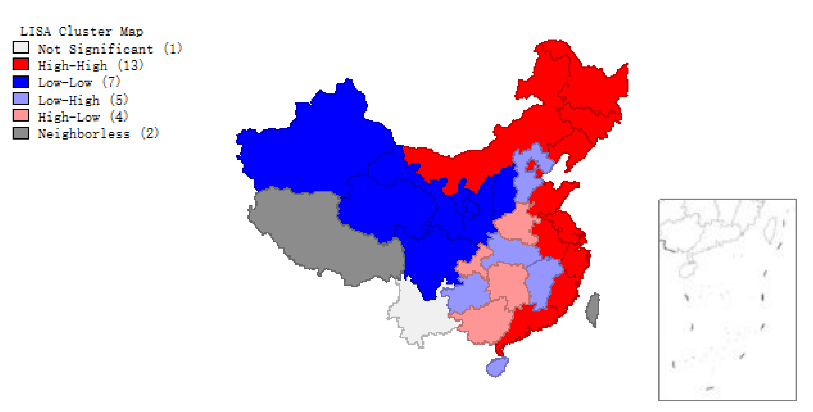
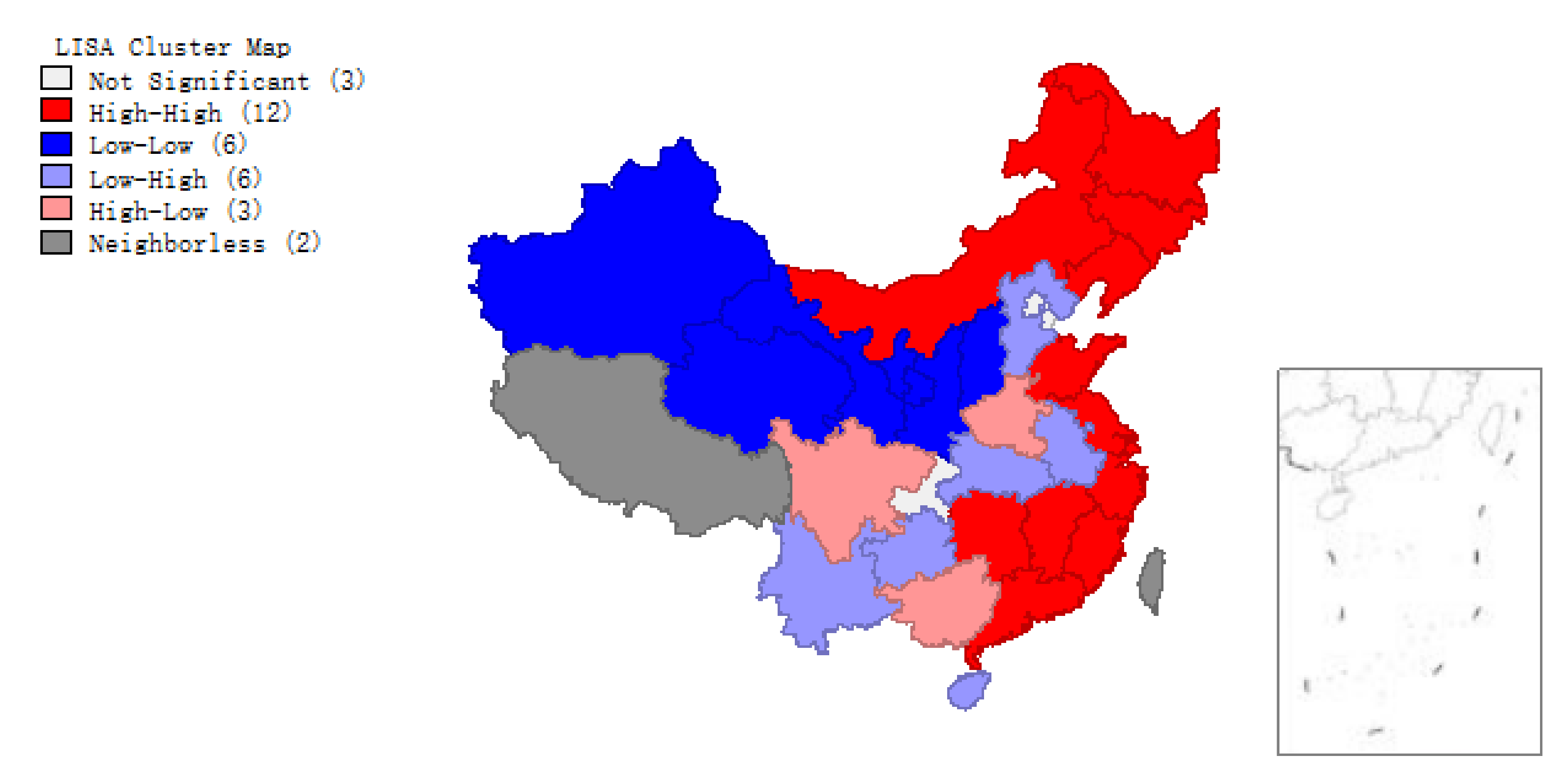
Global spatial autocorrelation analysis yields only one statistic to summarize the whole study area. One statistic is not enough to describe the details of individual regions. One way is to study the local spatial autocorrelation of local regions. The local indicators of spatial association (LISA) to evaluate the clustering in those individual units by calculating Local $Mora{n}^{’}sI$ for each spatial unit and evaluating the statistical significance for the i-th region:

$$I_i=\frac{{\sum }_{j=1}^n{w}_{ij}(x_j-\overline{x})(x_i-\overline{x})}{S^2}.$$

2.2. Spatial Quantile Autoregressive Model

Based on Su and Yang’s research [22] on the spatial quantile autoregressive model under cross-section data, we extend it to the panel data case. Combining the spatial autoregressive model with quantile regression method, we need to deal with endogenous issues. We use the instrumental variable method proposed by Chernozhukov and Hansen [23,24] to solve the variable endogenous problem, and give the process of parameter estimation of the spatial quantile autoregressive model.

In 1978, Koenker and Bassett [16] proposed the idea of quantile regression and extended the mean regression model to the quantile one.

Let $(\Omega ,\mathcal{F},P)$ be a probability space, Y a random variable defined in $\Omega$. For any real number y, the distribution function of the random variable Y is defined by $F\left(y\right)=P(Y\le y)$. For any $0\le \tau \le 1$, $Q^{\left(\tau \right)}\left(Y\right):=inf\{y:F\left(y\right)\ge \tau \}$ is called the $\tau$-th quantile of Y. $Q^{\left(\tau \right)}\left(Y\right)$ is abbreviated as $Q^{\left(\tau \right)}$. $Q^{\left(\tau \right)}$ can be seen as a function of $\tau$, called the quantile function of Y. Particularly, $Q^{\left(0.5\right)}$ is the median of Y.

The multivariate quantile regression model is defined as follows:

$$\begin{array}{c}\hfill Y=X{\beta }^{\left(\tau \right)}+U^{\left(\tau \right)},\end{array}$$

(8)

where $Y={(y_1,\cdots ,y_n)}^{\prime }$ with dependent components. $X={\left(x_{ij}\right)}_{n\times m}={(X_1,\cdots ,X_n)}^{\prime }$ is a non-random explanatory matrix, where the transpose ’′‘ follows the transpose rules of the block matrix. For each $i=1,\cdots ,n$, $X_i={(x_{i1},\cdots ,x_{im})}^{\prime }$. ${\beta }^{\left(\tau \right)}={({\beta }_1^{\left(\tau \right)},\cdots ,{\beta }_m^{\left(\tau \right)})}^{\prime }$ is the parameter vector to be estimated. $U^{\left(\tau \right)}={(u_1^{\left(\tau \right)},u_2^{\left(\tau \right)},\cdots ,u_n^{\left(\tau \right)})}^{\prime }$ is the error term. Assume each error component $u_i^{\left(\tau \right)}=y_i-X_i^{\prime }{\beta }_i^{\left(\tau \right)}$ satisfying the condition

$$\begin{array}{c}\hfill P(u_i^{\left(\tau \right)}\le 0|X_i)=\tau ,i=1,2,\cdots ,n,\end{array}$$

(9)

the formulas (9) mean that the conditional $\tau$-quantile of each error term is 0.

In 1973, Cliff and Ord [25] proposed a spatial autoregressive model. For the cross-sectional data, the spatial autoregressive model is expressed as:

$$\begin{array}{c}\hfill y_i=\lambda \sum _{j=1}^n{w}_{ij}{y}_j+X_i^{\prime }\beta +u_i,i=1,2,\cdots ,n,\end{array}$$

(10)

where the subscript i is the cross section unit. $y_i$ is the explained variable of the i-th cross section unit, and $X_i={(x_{i1},x_{i2},\cdots ,x_{im})}^{\prime }$ is the explanatory vector. $w_{ij}$ is the weight, reflecting the relation between the i-th region and the j-th region. Denote $Y={(y_1,\cdots ,y_n)}^{\prime }$, $W={\left(w_{ij}\right)}_{n\times n}$, $X={\left(x_{ij}\right)}_{n\times m}$, $\beta ={({\beta }_1,\cdots ,{\beta }_m)}^{\prime }$. $U={(u_1,\cdots ,u_n)}^{\prime }$ is the random error vector of independent and identically distributed with zero mean. The model (10) can be written in matrix form as follows:

$$\begin{array}{c}\hfill Y=\lambda WY+X\beta +U.\end{array}$$

(11)

By applying the first-order moment constraint $E\left(u_i\right|X_i)=0(i=1,2,\cdots ,n)$ to Equation (10), then the conditional mean $E(y_i-\lambda d_i|X)=x_i\beta$, where $d_i={\sum }_{i=j}^n{w}_{ij}{y}_j$. Similarly, applying quantile constraint $P(u_i^{\left(\tau \right)}\le 0|X)=\tau$ to Equation (10), the following Equation (12) can be obtained:

$$\begin{array}{c}\hfill P(y_i-{\lambda }^{\left(\tau \right)}{d}_i-X_i^{\prime }{\beta }^{\left(\tau \right)}\le 0|X_i)=\tau .\end{array}$$

(12)

Combining formula in (10) and (12), we have the spatial quantile autoregressive model for the cross-sectional data as follows:

$$\begin{array}{cc}\hfill y_i={\lambda }^{\left(\tau \right)}{d}_i+X_i^{\prime }{\beta }^{\left(\tau \right)}& +u_i^{\left(\tau \right)}\hfill \\ \hfill P(y_i-{\lambda }^{\left(\tau \right)}{d}_i-X_i^{\prime }{\beta }^{\left(\tau \right)}\le 0|X_i)& =\tau ,i=1,2,\cdots ,n.\hfill \end{array}$$

(13)

We extend model (13) to the spatial quantile autoregressive model for panel data:

$$\begin{array}{c}\hfill y_{it}={\lambda }^{\left(\tau \right)}{d}_{it}+X_{it}^{\prime }{\beta }^{\left(\tau \right)}+u_{it}^{\left(\tau \right)}\\ \hfill P(y_{it}-{\lambda }^{\left(\tau \right)}{d}_{it}-X_{it}^{\prime }{\beta }^{\left(\tau \right)}\le 0|X_{it})=\tau \\ \hfill i=1,2,\cdots ,n,t=1,2,\cdots ,T(\ge 1),\end{array}$$

(14)

where $X_{it}$ is an m-dimensional column vector.

Note: t can also be continuous time. Here we only consider the discrete case. We assume the time is divided into T periods. For each i and t, $(y_{it},X_{it})\in \mathbb{R}\times {\mathbb{R}}^m$ ($\mathbb{R}$ is the set of all real numbers, ${\mathbb{R}}^m$ is the m-dimensional Euclidean space). $d_{it}={\sum }_{j=1}^n{w}_{ij}{y}_{jt}$, ${\lambda }^{\left(\tau \right)}$ is the coefficient of the spatial lagged factor. ${\beta }^{\left(\tau \right)}$ is an $m\times 1$ vector of regression coefficients, $u_{it}\in \mathbb{R}$ is the error term with zero quantile, $X_{it}^{\prime }=(x_{i1t},x_{i2t},\cdots ,x_{imt})$.

Endogenous variables are important in economic modeling, which are determined by their relationship with other variables within the model and show whether a variable causes a particular effect. The spatial lagged factor $d_{it}={\sum }_{j=1}^n{w}_{ij}{y}_{jt}$ in the spatial autoregressive model can be regarded as an endogenous variable. The spatial econometric model combined with quantile regression needs to deal with endogenous issues. Otherwise, it will affect the accuracy of parameter estimation. Therefore, in the next subsection, we will discuss the instrumental variable method to deal with endogenous problems and parameter estimation.

2.3. Instrument Variable Method for Endogenous Problem and Parameter Estimation

Instrumental variables are variables that do not belong to the original model and are related to endogenous variables (Pearl, 2000 [26]). Concerning instrumental variable(IV) method, we refer to the literatures of Chernozhukov and Hansen [23,24], Matthew and Carlos (2009) [27].

Let ${\left(Z_i\right)}_{T\times m}={(Z_{i1},Z_{i2},\cdots ,Z_{iT})}^{\prime }$ be a matrix of instrument variables, where $Z_{it}^{\prime }=(Z_{i1t},Z_{i2t},\cdots ,Z_{imt})\in {\mathbb{R}}^m$. $Z_{it}$ is related to $X_{it}$ but unrelated to $u_{it}$ and satisfies

$$\begin{array}{c}\hfill P(y_{it}\le {\lambda }^{\left(\tau \right)}{d}_{it}+X_{it}^{\prime }{\beta }^{\left(\tau \right)}|X_{it},Z_{it})=\tau ,\end{array}$$

(15)

Let $\tilde{W}=I_T\otimes W$, where $I_T$ is the $T\times T$ identity matrix and ‘⊗’ represents the Kronecker product.

$$\begin{array}{cc}\hfill {\tilde{W}}_{nT\times nT}=I_T\otimes W& ={\left[\begin{array}{cccc}1& & & \\ & 1& & \\ & & \ddots & \\ & & & 1\end{array}\right]}_{T\times T}\otimes \left[\begin{array}{cccc}{w}_{11}& w_{12}& \cdots & w_{1n}\\ w_{21}& w_{22}& \cdots & w_{2n}\\ ⋮& ⋮& \ddots & ⋮\\ w_{n1}& w_{n2}& \cdots & w_{nn}\end{array}\right]\hfill \\ \hfill & =\left[\begin{array}{cccc}1\times W& & & \\ & 1\times W& & \\ & & \ddots & \\ & & & 1\times W\end{array}\right]\hfill \\ \hfill & =\left[\begin{array}{cccc}W& & & \\ & W& & \\ & & \ddots & \\ & & & W\end{array}\right]\hfill \end{array}$$

(16)

Take $Z_{it}={\sum }_{j=1}^n{\tilde{w}}_{ijt}{X}_{jt}$, where $X_{jt}^{\prime }=(X_{j1t},X_{j2t},\cdots ,X_{jmt})$, ${\tilde{w}}_{ijt}=w_{ij}$ for $t=1,\cdots ,T$, which implies the spatial weights are invariable in different periods. Then $Z_{it}$ is strictly exogenous and related to endogenous variables. The IV method will be simpler if $y_{it},d_{it},X_i,Z_i$ are independently and identically distributed. Then (15) is equivalent to find $({\lambda }^{\left(\tau \right)},{\beta }^{\left(\tau \right)})$ such that zero is a solution to the ordinary quantile regression:

$$\begin{array}{c}\hfill 0\in \underset{g\in G}{argmin}E\left[{\rho }_{\tau }(y_{it}-{\lambda }^{\left(\tau \right)}{d}_{it}-X_{it}^{\prime }{\beta }^{\left(\tau \right)}-g(X_{it},Z_{it}))\right],\end{array}$$

(17)

where ${\rho }_{\tau }\left(\varphi \right)=[\tau -\chi (\varphi \le 0)]\varphi$. $\chi (·)$ is the indicator function. G is a class of measurable functions of $(X_{it},Z_{it})$. Let $D=I_T\otimes (I_n-{\lambda }^{\left(\tau \right)}W)$, there is $G=(I_T\otimes W)D^{-1}$. Here we assume G is defined as follows:

$$\begin{array}{c}\hfill G=\{g(X_{it},Z_{it})={\gamma }^{\prime }{Z}_{it},\gamma \in \Gamma \},\end{array}$$

(18)

where $\gamma$ is a column vector and $\Gamma \subset {\mathbb{R}}^m$. In order to solve the problem (17), we construct the weighted quantile regressive objective function as follows:

$$\begin{array}{c}\hfill Q_{\tau }(\lambda ,\beta ,\gamma )=\frac{1}{nT}\sum _{i=1}^n\sum _{t=1}^T{\rho }_{\tau }(y_{it}-\lambda d_{it}-X_{it}^{\prime }\beta -{\gamma }^{\prime }{Z}_{it}).\end{array}$$

(19)

By the results in [23], the principle to solve problem (17) is to find $\widehat{\lambda },\widehat{\beta }$ such that the instrument variable coefficient $\widehat{\gamma }$ is driven as close to zero as possible. Here we use the two-stage least squares on the objective function (18).

Assumptions:

(1)

$P(u_{it}\le 0)=\tau ,\forall i=1,2,\cdots ,n,t=1,2,\cdots ,T$.

(2)

For any t, $\underset{n\ge 1}{sup}\underset{1\le i\le n}{max}E\left|u_{it}\right|\le \overline{u}\le \infty$.

(3)

Given a value of $u_{it}$, the conditional distribution function $F(·|{\overline{u}}_{it})$ has a bounded continuous conditional probability density function $f(·|{\overline{u}}_{it})$. Where ${\overline{u}}_{it}={\sum }_{k\ne i}^n{\sum }_{t=1}^T{g}_{ikt}{u}_{kt}$, $g_{ikt}$ is the element of G.

(4)

X is non-random. Its absolute value is uniformly bounded and contains the intercept term.

(5)

The instrument variable Z is non-random with full column rank.

Let ${\xi }_{it}={(X_{it},Z_{it})}^{\prime }$. The algorithm of solving parameter estimation of the SQAR model are summarized as follows:

Step 1: for a given $\tau$, to perform a ordinary quantile regression on $y_{it}-\lambda d_{it}$ based on ${\xi }_{it}$ as follows:

$$\begin{array}{c}\hfill ({\widehat{\beta }}^{\left(\tau \right)}\left(\lambda \right),{\widehat{\gamma }}^{\left(\tau \right)}\left(\lambda \right))=\underset{(\beta ,\gamma )}{argmin}{Q}_{\tau }(\lambda ,\beta ,\gamma ).\end{array}$$

(20)

Step 2: minimize the value of ${\widehat{\gamma }}^{\left(\tau \right)}\left(\lambda \right)$, and then get the estimator of ${\lambda }^{\left(\tau \right)}$:

$$\begin{array}{c}\hfill {\widehat{\lambda }}^{\left(\tau \right)}=\underset{\lambda }{argmin}{\widehat{\gamma }}^{\left(\tau \right)}\left(\lambda \right)\widehat{A}{\left({\widehat{\gamma }}^{\left(\tau \right)}\left(\lambda \right)\right)}^{\prime },\end{array}$$

(21)

where $\widehat{A}=A+o_p\left(1\right)$, $o_p\left(1\right)=\underset{\lambda }{sup}\left|\sqrt{n}{S}^{\left(\tau \right)}\left(\lambda \right)\right|$, $S^{\left(\tau \right)}\left(\lambda \right)=I_n-{\lambda }^{\left(\tau \right)}W$, A is a symmetric positive definite matrix. In fact, in order to find the estimator of ${\lambda }^{\left(\tau \right)}$, the coefficient ${\widehat{\gamma }}^{\left(\tau \right)}\left(\lambda \right)$ of the instrument variable should be driven as close to zero as possible. For simplicity, referring to the study of Chernozhukov and Hansen [23,24], here we take $\widehat{A}$ to be an identity matrix.

Step 3: performing weighted quantile regression on $y_{it}-{\widehat{\lambda }}^{\left(\tau \right)}{d}_{it}$ based on ${\xi }_{it}$ we can get an estimator of ${\beta }^{\left(\tau \right)}$:

$$\begin{array}{c}\hfill {\widehat{\beta }}^{\left(\tau \right)}={\widehat{\beta }}^{\left(\tau \right)}\left({\widehat{\lambda }}^{\left(\tau \right)}\right).\end{array}$$

(22)

3. Empirical Analysis and Results

In this section, we apply the above models to analyze the spatial autocorrelation and influence factors of energy efficiency of China during the years 1998–2016. Here we only consider 30 provinces and cities of China (Tibet, Hongkong, Macao and Taiwan were not studied in this paper since the incomplete data). All data come from China statistical Yearbook and local statistical Yearbooks (http://www.tjcn.org, http://data.stats.gov.cn). In the web page http://data.stats.gov.cn, one can find the navigation links to the annual reports of provinces. We downloaded and checked the data carefully. We assure the accuracy of input data in our models.

3.1. Spatial Autocorrelation Test Based on Global and Local $Mora{n}^{’}sI$

In [19], Lu and Zhang calculated energy efficiency according to (2) based on the low-carbon GDP output, where $n=30$, $m=3$ and $k=1$. Based on the results in [19], here we obtain yearly $Mora{n}^{’}sI$ and LISA during the study period 1998–2016. The spatial weight matrix is designed following the rook adjacency rule. Hainan province’s geographical location in China is special, an island across the sea from the mainland. There will be no neighbors under the rook adjacency method. However, since the reform and opening up, Hainan province has become increasingly close to the outside world. So we consider Hainan province to be adjacent to Guangdong province.

In statistics, there are p-value and Z-value or Z-score. The p-value is the probability that you have falsely rejected the null hypothesis. The Z-value is the measure of standard deviation. Very high or a very low (negative) Z-value, associated with very small p-values, are found in the tails of the normal distribution. It can be seen from

Table 1. $Mora{n}^{’}sI$ value of China of provincial energy efficiency.

Years	Moran’s I	p-Value	Z-Value
1998	0.319683	0.00568	2.8493
1999	0.310756	0.00611	2.7602
2000	0.291909	0.00847	2.6051
2001	0.304283	0.00680	2.7217
2002	0.329098	0.00405	2.9311
2003	0.391338	0.00086	3.8959
2004	0.387940	0.00099	3.8566
2005	0.370580	0.00133	3.6974
2006	0.377401	0.00116	3.7608
2007	0.370754	0.00132	3.7029
2008	0.382570	0.00107	3.8162
2009	0.346709	0.00219	3.4881
2010	0.366366	0.00152	3.6782
2011	0.400883	0.00072	4.0090
2012	0.394139	0.00088	3.9527
2013	0.370947	0.00142	3.7354
2014	0.369800	0.00136	3.7229
2015	0.356868	0.00162	3.5980
2016	0.349247	0.00186	3.5197

and Figure 1 that values of $Mora{n}^{’}sI$ of China’s provincial energy efficiency are positive. All $Mora{n}^{’}sI$ are statistically significant at the given significance level $1\%$. Therefore, it rejects the null hypothesis that there is no spatial autocorrelation in China’s provincial energy efficiency.

For each year, we obtained the scatter plots and clustering graphs of LISA. Here we only list the yearly results of 2008 and 2016 for limitation of pages.

It can be seen from Table 1 and Figure 1, the values of $Mora{n}^{’}sI$ are positive and fluctuate around 0.366 from 1998 to 2016, with little change year-on-year, which implies a positive correlation. On the whole, the energy efficiency $Mora{n}^{’}sI$ has a slight upward trend, and the spatial autocorrelation of energy efficiency is gradually increasing although the future trend is unclear.

The scatter plots of $Mora{n}^{’}sI$ (Figure 2 and Figure 3) and clustering graphs (Figure 4 and Figure 5) of LISA indicate that the spatial agglomeration of energy efficiency in China’s provinces tends to be stable. We can see that the energy efficiency of Chinese provinces is not randomly distributed. The energy efficiencies of regions with similar properties tend to gather together (High value of energy efficiency is adjacent to the high value of energy efficiency, low value of energy efficiency is adjacent to a low value of energy efficiency). The map is divided into four quadrants: The first quadrant (High-High) represents a space unit with a high energy efficiency value. Its neighboring provinces and cities are also high-efficiency units; The second quadrant (Low–High) represents the region with a low energy efficiency value. The energy efficiency values of its neighboring regions are at high level; the third quadrant (Low–Low) represents a low-energy efficiency space unit, and its neighboring provinces and cities are also low-efficiency units; The fourth quadrant (High–Low) represents a region with high energy efficiency value, but its neighboring region efficiency value is low.

Figure 1, Figure 2, Figure 3, Figure 4 and Figure 5 show that regions located in the first quadrant (High-High) are mainly the provinces and cities with higher economic development in the eastern coastal areas, such as Guangdong, Fujian, Zhejiang and Shanghai etc. The economic development of these provinces and cities is rapid. They have a positive influence on each other’s development. Provinces and cities in the third quadrant (Low–Low) are mainly distributed in northwest China such as Qinghai, Ningxia, Xinjiang, Gansu etc., where economic development is relatively backward with lower energy efficiency. The energy efficiency value of surrounding provinces and cities is also relatively low. Most provinces and cities in central China are located in the second quadrant (Low–High). In the fourth quadrant (High–Low) the energy efficiency values of various provinces and cities are interleaved, with little dependence on each other. Briefly, China’s provincial energy efficiency has obvious spatial autocorrelation. The energy efficiency value of a province is largely affected by the energy efficiency values of its neighboring provinces.

3.2. Influence Factors of Energy Efficiency

Base on results above, there are obvious spatial autocorrelation and spatial clustering phenomena in China’s provincial energy efficiency. The energy efficiency value of each province and city is affected by the neighboring regions’, which makes it reasonable to describe the data by a spatial autoregressive model. We take resource endowment (End), level of economic development (Eco), degree of government intervention (Gov), industrial structure (Ind), degree of opening to the outside world (Open), technical level (Tech) and energy prices (Price) as the main factors that affect energy efficiency. We use the spatial quantile autoregressive model (14) to analyze the influence of seven factors on energy efficiency values at the quantiles of $\tau =0.1,0.25,0.5,0.75,0.9$. Before build models, at first we preprocess the data set. For linear regression analysis, hypothesis testing on the data is necessary. Here we need to consider the multicollinearity of all explanatory variables. We also consider the heteroscedasticity of data. From Figure 6, we found that all explanatory variables have no multicollinaerity. The hypothesis test result in Figure 7 shows that the data are of heteroscedasticity, which implies that ordinary linear regression is invalid while quantile regression is a better tool to deal with the data with heteroscedasticity.

As a comparison, we also give the estimators based on ordinary spatial autoregression (10). The values of total-factor energy efficiency(TFEE) for application analysis come from the study of Lu and Zhang [19]. The variable description and data processing methods are given in

Table 2. Variable description of the spatial quantile autoregression (SQAR) model.

Variable Type	Variable	Data Processing Method
Explained Variable	TFEE	Calculated by DEA Model
	$End$	Energy production/Energy consumption
	$Eco$	Tertiary industry output/GDP $\times 100\%$
	$Gov$	Fiscal expenditure/GDP $\times 100\%$
Explanatory variables	$Ind$	Industrial output/GDP $\times 100\%$
	$Open$	Export trade volume/GDP $\times 100\%$
	$Tech$	Foreign direct investment/GDP
	$Price$	Price index of raw material, fuel and power(Base period is 1980)

:

We establish the SQAR model as follows (23):

$$\begin{array}{cc}\hfill TFE{E}_{it}& ={\lambda }^{\left(\tau \right)}{d}_{it}+{\beta }_0^{\left(\tau \right)}+{\beta }_1^{\left(\tau \right)}En{d}_{it}+{\beta }_2^{\left(\tau \right)}Ec{o}_{it}+{\beta }_3^{\left(\tau \right)}Go{v}_{it}\hfill \\ & +{\beta }_4^{\left(\tau \right)}In{d}_{it}+{\beta }_5^{\left(\tau \right)}Ope{n}_{it}+{\beta }_6^{\left(\tau \right)}Tec{h}_{it}+{\beta }_7^{\left(\tau \right)}Pric{e}_{it}+u_{it}^{\left(\tau \right)},\hfill \end{array}$$

(23)

where the subscripts $i(=1,\cdots ,30)$ and $t(=1,\cdots ,19)$ denote regions and years respectively. ${\beta }_l^{\left(\tau \right)}$$(l=1,2,\cdots ,7)$ are the parameters to be estimated. $u_{it}$ is the random error term. ${\lambda }^{\left(\tau \right)}$ is a coefficient of the spatial lagged factor $d_{it}={\sum }_{j=1}^n{w}_{ij}{y}_{jt}$. We treat $d_{it}={\sum }_{j=1}^n{w}_{ij}{y}_{jt}$ as an endogenous variable and select $Z_{it}$ that is defined in Section 2.3 as an instrumental variable. The parameters are estimated by using SQAR model at the following quantiles: $\tau =0.1,0.25,0.5,0.75,0.9$.

We use the software of Stata 12.0 to estimate parameters of the model SQAR based on the instrumental variables method given in Section 2.3. The formulas (20)–(22) are the algorithm about the parameter estimation of the model (23). For the sake of convenience to repeat the solving process based on our data, we give the operation process as follows:

• Computing the spatial effect $WY$, where W is the spatial weight matrix. The spatial weight matrix is designed following the rook adjacency rule. Y is the response variable (TFEE).
• Computing the instrumental variable $WX$, where W is the same weight matrix as the above and X is the matrix of explanatory variables.
• Open Stata version 12.0 and input: ivqreg EE eco gov ind tech end price(WY=WX),q($\tau$)
  For a given quantile $\tau$, we then can get the result of SQAR at the quantile.

In this work, we consider quantile $\tau =0.1,0.25,0.5,0.75,0.9$. The results are shown in

Table 3. Estimation results of the SQAR model, $\tau =0.1$.

Parameter	Estimate	p-Value	Z-Value	Standard Error	$95\%$ Confidence Interval
$\lambda$	−0.0792	0.000	−55.57	0.0014	[−0.0820,−0.0764]
${\beta }_0$	0.2263	0.006	2.72	0.0831	[0.0634,0.3892]
${\beta }_1$	−0.0323	0.000	−7.02	0.0046	[−0.0413,−0.0233]
${\beta }_2$	0.9629	0.000	6.63	0.1452	[0.6783,1,2474]
${\beta }_3$	−1.6151	0.000	−10.56	0.1529	[−1.9148,−1.3154]
${\beta }_4$	1.1177	0.000	7.67	0.1457	[0.8322,1.4032]
${\beta }_5$	0.1515	0.185	1.33	0.1142	[−0.0724,0.3754]
${\beta }_6$	−0.0097	0.792	−0.26	0.0367	[−0.0816,0.0622]
${\beta }_7$	−0.0788	0.016	−2.42	0.0326	[−0.1427,−0.0149]

,

Table 4. Estimation results of the SQAR model, $\tau =0.25$.

Parameter	Estimate	p-Value	Z-Value	Standard Error	$95\%$ Confidence Interval
$\lambda$	−0.0784	0.000	−82.99	0.0009	[−0.0729,−0.0695]
${\beta }_0$	0.4881	0.000	8.87	0.0550	[0.3803,0.5959]
${\beta }_1$	−0.0109	0.000	−3.59	0.0030	[−0.0169,−0.0050]
${\beta }_2$	0.6947	0.000	7.23	0.0960	[0.5065,0.8830]
${\beta }_3$	−1.2024	0.000	−11.89	0.1012	[−1.4006,−1.0041]
${\beta }_4$	1.0161	0.000	10.54	0.0964	[0.8272,1.2049]
${\beta }_5$	0.1075	0.155	1.42	0.0756	[−0.0406,0.2556]
${\beta }_6$	−0.0349	0.150	−1.44	0.0243	[−0.0825,0.0126]
${\beta }_7$	−0.0722	0.001	−3.35	0.0216	[−0.1145,−0.0300]

,

Table 5. Estimation results of the SQAR model, $\tau =0.5$.

Parameter	Estimate	p-Value	Z-Value	Standard Error	$95\%$ Confidence Interval
$\lambda$	−0.0712	0.000	−55.57	0.0014	[−0.0820,−0.0764]
${\beta }_0$	0.7620	0.000	15.21	0.0501	[0.6639,0.8602]
${\beta }_1$	−0.0024	0.393	−0.85	0.0028	[−0.0078,0.0031]
${\beta }_2$	0.3992	0.000	4.56	0.0875	[0.2278,0.5707]
${\beta }_3$	−1.0103	0.000	v10.97	0.0921	[−1.1908,−0.8297]
${\beta }_4$	0.6282	0.000	7.16	0.0878	[0.4563,0.8002]
${\beta }_5$	0.1272	0.064	1.85	0.0688	[−0.0077,0.2621]
${\beta }_6$	−0.0611	0.006	−2.76	0.0211	[−0.1044,−0.0178]
${\beta }_7$	0.0032	0.869	0.17	0.0186	[−0.0352,0.0417]

,

Table 6. Estimation results of the SQAR model, $\tau =0.75$.

Parameter	Estimate	p-Value	Z-Value	Standard Error	$95\%$ Confidence Interval
$\lambda$	−0.0444	0.000	−50.34	0.0009	[−0.0462,−0.0427]
${\beta }_0$	0.8337	0.000	16.19	0.0515	[0.7327,0.9346]
${\beta }_1$	−0.0053	0.064	−1.86	0.0028	[−0.0109,0.0003]
${\beta }_2$	0.3642	0.000	4.05	0.0899	[0.1879,0.5404]
${\beta }_3$	−0.8454	0.000	−8.92	0.0947	[−1.0310,−0.6597]
${\beta }_4$	0.3964	0.000	4.39	0.0902	[0.2196,0.5733]
${\beta }_5$	0.0488	0.490	0.69	0.0708	[−0.0899,0.1875]
${\beta }_6$	−0.0253	0.266	−1.11	0.0227	[−0.0698,0.0193]
${\beta }_7$	0.0068	0.738	0.33	0.0202	[−0.0328,0.0463]

and

Table 7. Estimation results of the SQAR model, $\tau =0.9$.

Parameter	Estimate	p-Value	Z-Value	Standard Error	$95\%$ Confidence Interval
$\lambda$	0.0033	0.002	3.08	0.0011	[0.0012,0.0055]
${\beta }_0$	0.8455	0.000	13.39	0.0632	[0.7217,0.9693]
${\beta }_1$	−0.0096	0.006	−2.74	0.0035	[−0.0164,−0.0027]
${\beta }_2$	0.2315	0.036	2.10	0.1103	[0.0153,0.4477]
${\beta }_3$	−0.6357	0.000	−5.47	0.1162	[−0.8634,−0.4080]
${\beta }_4$	0.2361	0.033	2.13	0.1107	[0.0192,0.4530]
${\beta }_5$	−0.6421	0.459	−0.74	0.0868	[−0.2343,0.1059]
${\beta }_6$	0.0334	0.068	1.83	0.0279	[−0.0212,0.0880]
${\beta }_7$	0.0089	0.720	0.36	0.0248	[−0.0396,0.0574]

.

From Table 3, Table 4, Table 5, Table 6 and Table 7, it can be seen that the spatial autoregressive coefficient $\lambda$ is significantly negative at $\tau \le 0.75$ and significantly positive for $\tau =0.9$ with the significant level 1%. This shows that at lower value of energy efficiency, the neighboring provinces and cities of a region have a negative influence on it, resulting in a low-low clustering case. Regions with higher energy efficiency tend to have a positive influence on the surrounding provinces and cities, which contributes to a high-high clustering distribution pattern. At the same time, this is also consistent with the conclusion of $Mora{n}^{’}sI>0$. While in the SAR model (

Table 8. Estimation results of the ordinary spatial autoregression (SAR) model.

Parameter	Estimate	p-Value	Z-Value	Standard Error	$95\%$ Confidence Interval
$\lambda$	0.3262	0.000	3.54	0.0921	[0.1457,0.5067]
${\beta }_0$	0.3627	0.000	3.83	0.0946	[0.1773,0.5481]
${\beta }_1$	−0.0013	0.426	−0.80	0.0016	[−0.0044,0.0018]
${\beta }_2$	0.1423	0.089	1.70	0.0836	[−0.0216,0.3061]
${\beta }_3$	−0.2722	0.014	−2.46	0.1105	[−0.4888,−0.0556]
${\beta }_4$	0.2542	0.060	1.88	0.1353	[−0.0111,0.5194]
${\beta }_5$	0.1210	0.250	1.15	0.1051	[−0.0850,0.3271]
${\beta }_6$	−0.0081	0.500	−0.67	0.0121	[−0.0317,0.0155]
${\beta }_7$	−0.0025	0.877	−0.14	0.0177	[−0.0371,0.0321]

), the spatial effect coefficient $\lambda =0.3262$ is significantly positive, and much bigger than that at quantile $0.9$ of SQAR model. Obviously, the estimate of spatial effect in SAR is rougher and somewhat unreasonable. The heteroscedasticity of data may explain why this happens.

Considering the influence factors, we obtain the following results:

• The coefficient of variable $End$ is negative at all quantiles. Except for at the quantile 0.5, the coefficient of variable $End$ is statistically significant at other quantiles. It shows that there is a negative correlation between the level of resource endowment and energy efficiency, that is, the situation of energy utilization efficiency in regions with more sufficient resource reserves is worse. The same result also can be obtained in the spatial autoregressive (SAR) model (See Table 8) but the p-value is 0.426, which means the negative influence of resource endowment level on energy efficiency is not statistically significant according to the result of SAR model. This shows that the regression results of the SAR model are not ideal.
• The estimates of the parameter of the variable $Eco$ are positive for all quantiles and the estimate is smaller at the upper quantile. This indicates that the level of economic development obviously promotes the improvement of energy efficiency, and with the increase of energy efficiency, the positive role of promotion is steadily weakening.
• The estimates ($\widehat{{\beta }_3}$) of the parameter of variable $Gov$ are significantly negative in SQAR model at all quantiles and in SAR model. The absolute values of estimates are smaller at the upper quantile. For example: $\tau =0.1,\widehat{{\beta }_3}=-1.6151$; $\tau =0.25,\widehat{{\beta }_3}=-1.2024$; $\tau =0.5,\widehat{{\beta }_3}=-1.0103$. This shows that the degree of government intervention has a negative correlation with energy efficiency. However, this negative influence gradually weakens as energy efficiency increases.
• The influence of industrial structure on energy efficiency is quite similar to the influence of economic development level on energy efficiency. The influence of industrial structure on energy efficiency is greater.
• When $\tau \le 0.75$, the degree of opening to the outside world has a positive effect on energy efficiency. while $\tau =0.9$, the degree of opening to the outside has a negative effect on energy efficiency. The results of the SAR model show that there is a positive correlation between the degree of opening to the outside world and energy efficiency. Compared with the SQAR model, the conclusion shown by the SAR model is somewhat limited. It can not describe the full information. This also exposes the disadvantages of ordinary mean regression.
• At lower quantile of energy efficiency $(\tau \le 0.5)$, there is a negative correlation between the level of technological development and energy efficiency, and the negative correlation at quantile 0.5 is most significant. At a higher quantile of energy efficiency, the effect of the technical level is positive and statistically significant at the 10% level. However, the SAR model shows that the technical level has a negative influence on energy efficiency. Obviously, the SAR model hides the tail information of the data. So the result of the SAR model can not fully describe the true distribution of data.
• When $\tau \le 0.25$, the estimates of the parameter of $Price$ are significantly negative, indicating that at a lower level of energy efficiency, the higher the energy price the lower the energy efficiency value. When $\tau \ge 0.5$, energy prices have a positive effect on energy efficiency.

3.3. Conclusions

Through the empirical analysis to the energy efficiency of Chinese 30 provinces and cities at different quantiles, we draw conclusion as follows.

The level of economic development and industrial structure have a significant role in promoting energy efficiency. There is a negative correlation between resource endowment and energy efficiency. The degree of opening to the outside world has no significant influence on energy efficiency. Only at a high level of energy efficiency can the technical level play a certain role in promoting. At a lower energy efficiency level, energy price has a significant negative influence on energy efficiency. By comparing with an ordinary spatial autoregressive model, this paper shows the advantages of spatial quantile autoregressive modes in the analysis process. SQAR model is more resistant to outliers and can describe the statistical distribution of variables in more detail.

Based on the above analysis, We offer a few suggestions that will help to promote energy efficiency.

• Improve the economic level of each province and optimize the industrial structure. The government at all levels should take measures to allocate resources reasonably. China’s resources are concentrated in the central and western regions. These regions have unique resource conditions but the economic level is generally low. The government’s fiscal expenditure cannot play an active role. Therefore, the government needs to properly adjust the intensity of government intervention and allocate resources to promote the improvement of energy efficiency.
• Provinces and cities with lower energy efficiency should put economic development and optimization of industrial structure in the first place. Regions with higher energy efficiency may continue to accelerate technological development. Under the lower efficiency level, both the technical level and the energy price have a negative influence on energy efficiency. At this time, rushing to raise the technical level and lowering the energy price may not help. So only by solving the most basic problem—economic development—can the development of other aspects be driven. For provinces and cities with higher energy efficiency, they have strong economic strength and a reasonable industrial structure. So it is better to develop and innovate science and technology constantly, making science and technology a powerful driving force for improving energy efficiency.

4. Discussion

The practical world is complex. In order to model the real world by using quantitative methods such as statistics tools, we have to make some assumptions in advance. For example, for ordinary linear regression, normal distribution and homoscedasticity are required. While, if the data does not follow a normal distribution and has heteroscedasticity, quantile regression is a good option. Compared with the existing references related to the analysis of factors influencing energy efficiency, the novelty of our model (23) is that it considers not only the spatial correlation of energy efficiency but also the heteroscedasticity of explanatory variables. Given a quantile $\tau$ and the input data of explanatory variables X in model (23), the output is the conditional quantile of efficiency under given X. It can characterize the distribution of energy efficiency. However, for ordinary regression, the output is the mean of energy efficiency, which is a rougher estimate. For example, given $\tau =0.25$, input the data of Hubei province in 2016, we get the output 0.683 of model (23). That means when the values of explanatory variables change, the quantile at 0.25 of energy efficiency of Hubei is 0.683. Considering the energy of efficiency in the period of 1998–2016 of Hubei province, we get the 0.25 quantile is 0.687. The fitting effect is not bad from this single case. However, it does not mean our model is complete. The result of our model can not perfectly explain the practical world since it is based on some assumptions, although it is expected helpful to improve the energy efficiency for decision-makers for maintaining the sustainability of social development. It still needs to be improved. Here we only considered the spatial lagged effect and ignored the time-lagged effect. In our future work, based on the quantile method, we will consider both spatial lagged effect and time-lagged effect, i.e., consider the dynamic panel data.

References

1. Ayres, R.U.; Turton, H.; Casten, T. Energy efficiency, sustainability and economic growth. Energy 2007, 32, 634–648. [Google Scholar]
2. Mavi, N.K.; Mavi, R.K. Energy and environmental efficiency of OECD countries in the context of the circular economy: Common weight analysis for malmquist productivity. J. Environ. Manag. 2019, 247, 651–661. [Google Scholar]
3. Miketa, A. Analysis of energy intensity developments in manufacturing sectors in industrialized and developing countries. Energy Policy 2001, 29, 769–775. [Google Scholar]
4. Yu, X.; Moreno-Cruz, J.; Crittenden, J.C. Regional energy rebound effect:The impact of economy-wide and sector level energy efficiency improvement in Georgia, USA. Energy Policy 2015, 87, 250–259. [Google Scholar]
5. Zheng, J.; Mi, Z.; Coffman, D.M.; Milcheva, S.; Shan, Y.; Guan, D.; Wang, S. Regional development and carbon emissions in China. Energy Econ. 2019, 81, 25–36. [Google Scholar]
6. Tobler, W.R. A computer movie simulating urban growth in the detroit region. Econ. Geogr. 1970, 46, 234–240. [Google Scholar]
7. Shen, N.; Liu, F. Spatial spillover, threshold characteristics and the economic growth effect of energy efficiency. China Popul. Resour. Environ. 2012, 5, 155–159. [Google Scholar]
8. Makridou, G.; Andriosopoulos, K.; Doumpos, M.; Zopounidis, C. Measuring the efficiency of energy-intensive industries across European countries. Energy Policy 2016, 88, 573–583. [Google Scholar]
9. Li, H.; Shi, J.F. Energy efficiency analysis on Chinese industrial sectors: An improved Super-SBM model with undesirable outputs. J. Clean. Prod. 2014, 65, 97–107. [Google Scholar]
10. Liu, J.; Mao, J. Analysis of China’s provincial energy efficiency distribution and its influencing factors based on spatial measurement. J. Hunan Univ. Financ. Econ. 2014, 30, 133–140. [Google Scholar]
11. Gao, Z.; Wang, Y. Regional division of energy productivity in China and analysis of influencing factors. J. Quant. Tech. Econ. 2006, 9, 46–57. [Google Scholar]
12. Jiang, L.; Folmer, H.; Ji, M.; Tang, J. Energy efficiency in the Chinese provinces: A fixed effects stochastic frontier spatial Durbin error panel analysis. Ann. Reg. Sci. 2017, 58, 301–319. [Google Scholar]
13. Li, K.; Lin, B. How to promote energy efficiency through technological progress in China? Energy 2018, 143, 812–821. [Google Scholar]
14. Qiu, L.; Shen, Y.; Ren, W.; Yan, T. Regional differentiation and influencing factors analysis of energy efficiency in China. J. Nat. Resour. 2008, 23, 920–928. [Google Scholar]
15. Zou, Y.; Lu, Y. Analysis of regional characteristics of energy efficiency in China based on spatial autoregressive model. Stat. Res. 2005, 10, 67–71. [Google Scholar]
16. Koenker, R.; Bassett, G. Regression quantiles. Econometrica 1978, 46, 33–50. [Google Scholar]
17. Koenker, R. Quantile regression for longitudinal data. J. Multivar. Anal. 2004, 91, 74–89. [Google Scholar]
18. McMillen, D.P. Quantile Regression for Spatial Data; Springer: Berlin/Heidelberg, Germany, 2012. [Google Scholar]
19. Lu, Q.; Zhang, J. Analysis of total-factor energy efficiency in China under low carbon constraint. In Proceedings of the 5th International Conference on Big Data and Information Analytics, Kunming, China, 8–10 July 2019. [Google Scholar]
20. Moran, P.A.P. Notes on continuous stochastic phenomena. Biometrika 1950, 37, 17–23. [Google Scholar]
21. Charnes, A.; Cooper, W.W.; Rhodes, E. Measuring the efficiency of decision making units. Eur. J. Oper. Res. 1978, 2, 429–444. [Google Scholar]
22. Su, L.; Yang, Z. Research Collection School of Economics. Instrumental Variable Quantile Estimation of Spatial Autoregressive Models. Working paper. May 2011, pp. 1–35. Available online: https://ink.library.smu.edu.sg/soe_research/1074 (accessed on 12 January 2021).
23. Chernozhukov, V.; Hansen, C. Instrumental quantile regression inference for structural and treatment effect models. J. Econom. 2006, 132, 491–525. [Google Scholar]
24. Chernozhukov, V.; Hansen, C. Instrumental variable quantile regression: A robust inference approach. J. Econom. 2008, 142, 379–398. [Google Scholar]
25. Paul Elhorst, J. Spatial Econometrics: From Cross-Sectional Data to Spatial Panels; Springer: Berlin/Heidelberg, Germany, 2014. [Google Scholar]
26. Pearl, J. Causality: Models, Reasoning, and Inference; Cambridge University Press: Cambridge, UK, 2000. [Google Scholar]
27. Matthew, H.; Carlos, L. A quantile regression approach for estimating panel data models using instrument variables. Econ. Lett. 2009, 104, 133–135. [Google Scholar]
Figure 1. Trend of M o r a n s I .
Energies 14 00504 g001
Figure 2. Scatter plot of M o r a n s I of provincial energy efficiency, 2008.
Energies 14 00504 g002
Figure 3. Scatter plot of M o r a n s I of provincial energy efficiency, 2016.
Energies 14 00504 g003
Figure 4. Local indicators of spatial association (LISA) of provincial energy efficiency, 2008.
Energies 14 00504 g004
Figure 5. LISA of provincial energy efficiency, 2016.
Energies 14 00504 g005
Figure 6. Multicollinearity test.
Energies 14 00504 g006
Figure 7. Heteroscedasticity test.
Energies 14 00504 g007