Mitigating the Piston Effect in High-Speed Hyperloop Transportation: A Study on the Use of Aerofoils

Abstract

The Hyperloop is a concept for the high-speed ground transportation of passengers traveling in pods at transonic speeds in a partially evacuated tube. It consists of a low-pressure tube with capsules traveling at both low and high speeds throughout the length of the tube. When a high-speed system travels through a low-pressure tube with a constrained diameter such as in the case of the Hyperloop, it becomes an aerodynamically challenging problem. Airflow tends to get choked at the constrained areas around the pod, creating a high-pressure region at the front of the pod, a phenomenon referred to as the “piston effect.” Papers exploring potential solutions for the piston effect are scarce. In this study, using the Reynolds-Average Navier–Stokes (RANS) technique for three-dimensional computational analysis, the aerodynamic performance of a Hyperloop pod inside a vacuum tube is studied. Further, aerofoil-shaped fins are added to the aeroshell as a potential way to mitigate the piston effect. The results show that the addition of fins helps in reducing the drag and eddy currents while providing a positive lift to the pod. Further, these fins are found to be effective in reducing the pressure build-up at the front of the pod.

1. Introduction

The twentieth-century transport systems have been ruled by oil-fueled cars, trucks, and planes. The global transportation of today is in need of new and disruptive transportation technologies due to increasing air quality concerns, global climate change, and the desire for energy efficiency and sustainability [1]. In 1909, rocket pioneer Robert H. Goddard proposed the first concept of high-speed trains moving in vacuum or evacuated tubes [2], an idea that was patented after his death [3]. Bachelet introduced the core idea of levitating trains in 1912 [4]. Over the years, these concepts and ideas were refined further. Currently, trains commonly known as “High-Speed Rail” (HSR) achieve speeds close to 300 mph [5]. Hyperloop is being perceived as a potential alternative for HSR and air passenger transport systems for long-distance passenger transport [6].

The concept of high-speed transportation using Hyperloop has been gaining attention in the recent years. The concept was originally proposed by Elon Musk in a white paper published by SpaceX in 2013 [7] as a quicker and efficient form for short-haul travel. The system consists of a low-pressure tube with capsules traveling at both low and high speeds throughout the length of the tube using levitation [8]. The time spent traveling during short journeys at cruise speed is much lower compared to the overall end-to-end travel time in air transportation due to the inefficiencies in air travel (runway taxiing, climb, descent, etc.) [9]. For example, to travel from San Francisco to Los Angeles (a distance of 559 km), a typical aircraft’s gate-to-gate travel time is 1 h and 28 min; however, the actual time that the aircraft spends for flying is 58 min and the remaining 30 min are used for taxiing, take off, landing, and arrival at the gate. The Hyperloop pods could alleviate some of these inefficiencies by traveling in near-vacuum conditions, allowing them to maintain much higher speeds. Furthermore, the Hyperloop concept can also alleviate some pressure on increasingly congested airports and flight routes and is projected to grow rapidly over the next few decades.

While designing high-speed transportation systems, a critical factor that determines the energy consumption by the system is the aerodynamics of the vehicle. The “piston effect” is an aerodynamic issue that is recognized by researchers while designing vehicles passing through enclosed spaces such as tunnels. As a vehicle such as a high-speed train or the Hyperloop pod travels through a tunnel, the walls around the vehicle form a space constraint and restrict the airflow around the profile of the vehicle [10]. This leads to a pressure buildup at the front of the vehicle and creates an effect similar to the pressure increase inside a mechanical plunger. This effect is termed as the “piston effect” or the “plunger effect” [11]. In addition, the viscous fluid around the vehicle creates a drag force known as the “skin drag.”

In a railway tunnel, as trains have a large cross-sectional area and almost completely fill the tunnel, the piston effect is largely noticeable. The piston effect is caused by the narrow gap between the outer surface of the vehicle and the wall of the constrained path. At high speeds, the flow gets choked at these narrow spaces, creating a pressure build-up at the front (Figure 1). Road vehicle tunnels do not have that much effect, as the cross-sectional area of the vehicle is very small in comparison with that of the tunnel. A maximum effect can be seen in single-track tunnels between the rolling stock and the tunnel and is affected by the shape of the front of the train [12].

In some underground rapid transit systems, the airflow around the vehicle contributes to the ventilation of the vehicle and also makes mechanical ventilation unnecessary by providing enough air movement. Air quality remains the same or can even improve at wider stations with multiple tracks. However, at narrow single tunnels, the air quality worsens when relying only on the plunger effect for ventilation [13].

“Tunnel boom” is another phenomenon associated with high-speed vehicles in constrained spaces. When a high-speed train exit tunnels, a loud sound is generated due to the sudden expansion of the compressed air in front of the vehicle and the resulting creation of shock waves. The shock waves can damage the strength and structure of the pod and negatively affect its aerodynamic performance [12]. The strength of this wave is proportional to the cube of the pod’s speed [13].

As the presence of the plunger effect creates a significant drag on the transportation pod, reducing the effect of this effect is of significant concern when it comes to the energy required to operate the vehicle. The objective of this study is to demonstrate the presence of the plunger effect in a Hyperloop pod using three-dimensional computational fluid dynamics (CFD) models and to devise a technique to reduce the adverse effects of the same.

1.1. Studies on Airflow around High-Speed Systems

While studies on the airflow around a Hyperloop pod are scarce, there is extensive literature available on other high-speed bodies. The closest example is the high-speed train. Several studies have used experimental setups to study the airflow pattern around trains in an open environment, e.g., [14,15,16,17], when a wall interference is present [18] and in constrained spaces such as tunnels [19,20,21]. However, the experimental setup to study the airflow around a train or a Hyperloop system is expensive and the experimentation is time- and labor-intensive. Due to this reason, several recent studies have relied on various computational techniques to simulate the airflow pattern and study various flow parameters. All these studies have generated accurate results in comparison with the experimental results.

Reynolds-Averaged Navier–Stokes (RANS) has been one of the most popular computational techniques used by researchers in recent times. It has been used very frequently to study the aerodynamics of a high-speed train in an open environment and has been proven as an accurate method [22,23]. There have been a few studies on the motion of trains through constrained spaces using RANS. For example, Shin and Park [24] illustrated that a vortex was formed in front of the train as it entered the tunnel and the airflow pattern generated a significant drag. In 2011, Li et al. [25] showed that the pressure generation at the front of the train due to the vortex formation was proportional to the square of the train’s speed. Further studies have explored more complicated pressure patterns generated inside a tunnel when more than one train moves through it [26,27].

Several studies in the literature have used other computational modeling techniques to understand airflow around high-speed systems. Large Eddy Simulation (LES) is a technique that was introduced in 1962 [28] and is very popular in modeling turbulent flows [29,30,31,32]. Detached Eddy Simulation (DES) is another technique that is used for more complex flow situations such as the study of a wake region behind trains traveling at high speeds, e.g., [33,34,35]. In 2012, Mei et al. [36] used the Riemann variables method to predict the pressure waves generated by a high-speed train inside a tunnel. Apart from this study, a majority of computational studies on high-speed systems in constrained spaces rely on the RANS method.

To resolve the smallest turbulent phenomena and fastest fluctuations, Direct Numerical Simulation (DNS) can be employed, which uses a very fine mesh and very small time steps. Without additional modeling, this approach can resolve turbulence. The computational cost of DNS is high for resolving turbulence for high Reynolds numbers in complex geometries, but it is a very reliable method. Large-eddy simulation (LES), detached eddy simulation (DES), and steady and unsteady RANS methods are available modeling techniques for turbulence flows. In this study, the unsteady RANS model is employed.

1.2. Kantrowitz Limit

The Kantrowitz Limit is a relevant limiting condition for designing a transport system that is expected to work inside a constrained space within a transonic or supersonic velocity regime [37]. It determines the stalling condition of a gas flow at transonic speeds flowing through a narrow path. When there is an area reduction in the flow of the fluid, the flow speeds up in order to maintain the same mass flow rate, as per the continuity equation. When the flow is supersonic, when it experiences an area contraction, the flow gets choked as the velocity of the flow increases until it reaches the local speed of sound. The Kantrowitz limit represents the maximum amount of compression a flow experiences before it chokes—the speed of the flow can no longer be increased more than this limit and cannot be influenced by the upstream or downstream pressure changes.

The Kantrowitz limit is a crucial factor when studying the aeroshell design of a Hyperloop pod. As Hyperloop pods are sealed and move through a near-vacuum tube at high-subsonic speeds, the flow gets choked easily when the Kantrowitz limit is met, increasing the possibility of the piston effect.

1.3. Aerodynamic Studies on the Hyperloop

One of the first published studies on the aerodynamics of the Hyperloop pod is from Chin et al. [38]. They used analytical calculations to understand the pressure distribution around the pod. Based on their one-dimensional analysis, the authors concluded that it was difficult to achieve high speeds as proposed by Musk [7] with the proposed dimensions due to the high pressure in the tube as the pod achieved high speeds. A perceived solution for this situation included pumping the air out of the tube, which was considered a nonviable option for long-distance transportation.

In 2017, Braun et al. [39] used computational techniques to design and optimize the aerodynamic performance of their Hyperloop pod. They used a one-dimensional analysis through a reduced-flow model and a multi-objective optimization along with a three-dimensional CFD solver. Their two design objectives were the increase in lift and reduction in drag. In the same year, Yang et al. [40] conducted an aerodynamic study on their Hyperloop pod using $\mathrm{k}-\omega SST$ modeling and found that the speed of the pod and the pressure inside the tube were two critical parameters that affected the aerodynamic drag on the pod. They explored the use of a suction mechanism and an on-board air-compressor and found that a combination of these two could help in reducing the drag to an extent.

In 2018, Opgenoord and Caplan [9] performed an aerodynamic analysis of their Hyperloop pod using two-dimensional computational techniques. The aim of the study was to see how the Hyperloop pod that the MIT team designed for the SpaceX Hyperloop Competition behaved aerodynamically under various speeds. They studied the pod under a tube pressure of 860 Pa as compared to the 25 Pa proposed in the whitepaper from Musk [7]. They studied the performance of the pod at Mach numbers of 0.32, 0.65, 0.675, and 0.7. They used a laminar Navier–Stokes method for M = 0.32 and the k-⍵ SST turbulence model for larger speeds. The authors observed that there was a small increase in the drag from M = 0.5 to 0.65 as the flow turned supersonic at the highest point of the pod, resulting in a small shock. The flow started choking at around M = 0.675 and the drag increase was larger for higher Mach numbers. At M = 0.8, the drag coefficient was three times that of M = 0.65 as the speed increased past the Kantrowitz limit.

More recently, Oh et al. [41] used a two-dimensional RANS model to study the aerodynamics of their Hyperloop pod. They observed the pressure build-up at the front of the pod at high speeds. Further, they studied the effects of the blockage ratio, pod length, temperature, and tube pressure on the aerodynamic drag experienced by the pod.

In this study, our objective is to understand the aerodynamic performance of a Hyperloop pod under the tube pressure and conditions suggested by Musk’s white paper [7] and to devise a technique to reduce the drag experienced by the pod. While the previous studies have explored the choking of air flow around the pod and the pressure build-up at the front as a result (the piston effect), the Yang et al. paper [40] is the only one that recommended a solution to reduce these effects (apart from profile optimization). In this paper, we propose and investigate the use of aerofoil-shaped external fins as a potential solution to optimize the air flow around the pod. We use a three-dimensional CFD model based on RANS and the turbulent flow is simulated using the Direct Numerical Simulation (DNS) technique.

1.4. Research Questions

In this paper, we investigate the following specific questions related to the aerodynamic performance of a Hyperloop pod:

• How does the piston effect influence the performance of a Hyperloop pod in a partially vacuum tunnel?
• Does the addition of aerofoil-shaped fins improve the aerodynamic performance of a Hyperloop pod?

2. Method

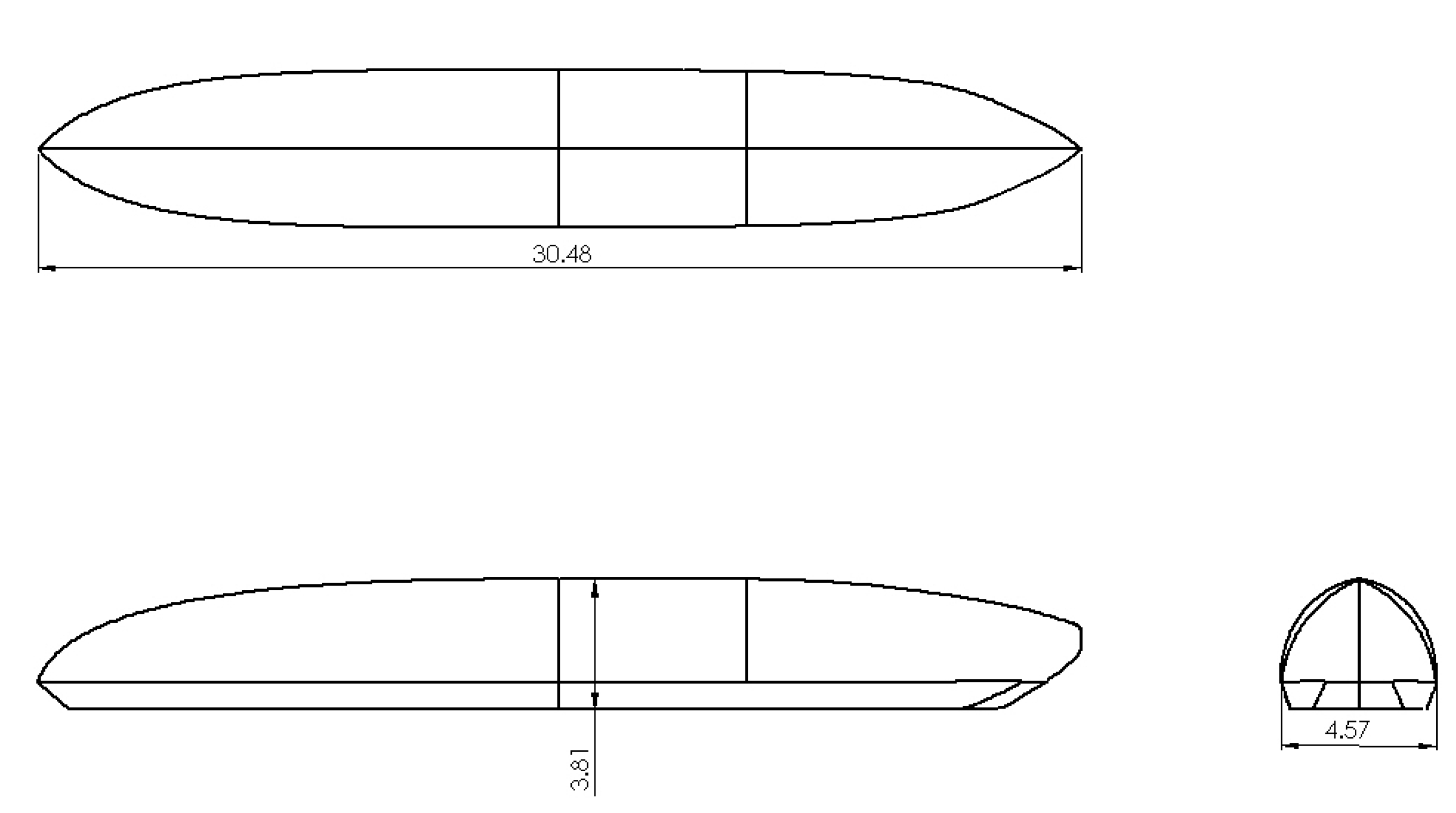
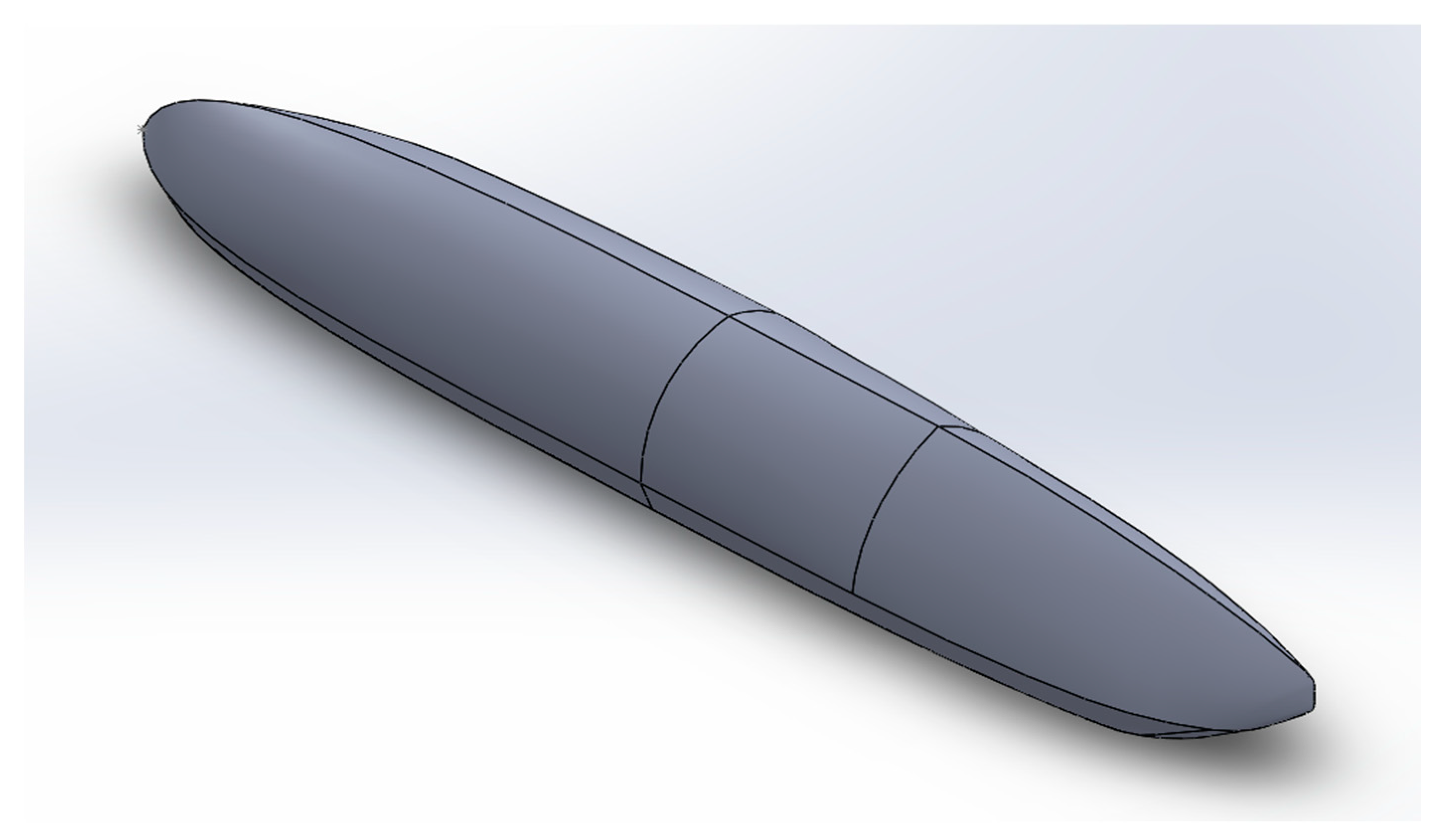
2.1. Model Dimensions

The study described in this paper is conducted on the aeroshell modeled by the Spartan Hyperloop student team from San Jose State University (SJSU), a team that regularly participated in SpaceX’s Hyperloop pod competition. The team has developed a design for the aeroshell using CFD techniques and this shell has a reasonably low coefficient of drag in an open environment. This aeroshell has a three-piece modular design for ease of assembly and uses a slide-on latching and fastening mechanism to attach to the chassis of the pod. The design of the aeroshell is inspired by Maglev trains and Tesla’s Model 3. Figure 2 depicts the CAD model of the design used for the study. The study is performed on the full-scale passenger-size pod with overall dimensions of 30.5 m × 4.6 m × 3.8 m (100 ft. × 15 ft. × 12.5 ft.), as shown in Figure 3.

For the purpose of addressing the research questions, two different pods are considered in this paper. The first pod has overall dimensions of 30.5 m × 4.6 m × 3.8 m, which are the same as those of the aeroshell designed by the Spartan Hyperloop team. This pod does not have an attached aerofoil and it operates in a partially vacuum tube with a diameter of 5.2 m (17 ft.). This pod will be referred to as “phase 1 pod” further in this paper.

The second pod, referred to as “phase 2 pod” further, is similar to the phase 1 pod in dimensions. It has added aerofoil-shaped fins attached to its body. NASA LS (1)-0413 (GA(W)-2) has been used as the shape of the aerofoil. In order to accommodate the aerofoil, the tube diameter is increased to 5.3 m (17.5 ft.).

2.2. Computational Modeling

Based on the survey of existing literature, Reynolds-Averaged Navier–Stokes (RANS) is observed to be the most accurate computational technique to study the fluid flow in constrained spaces around a vehicle. The flow around the pod for our analysis is assumed to be compressible; thus, it is necessary to express the continuity and Navier–Stokes equations for incompressible flow as:

$$\frac{\partial \overline{\rho }}{\partial t}+\frac{\partial }{\partial x}\left(\overline{\rho }u\right)=0$$

(1)

where $\overline{\rho }$ represents the density of the fluid, u represents the flow velocity, t represents time, and x represents a space coordinate.

The unsteady RANS model is based on the decomposition of the flow parameters into a time-averaged and a fluctuating component. In this model, the continuity and Navier–Stokes equations take the forms shown in Equations (2) and (3):

$$\frac{\partial \overline{u_i}}{\partial x_i}=0$$

(2)

where $\overline{u_i}$ represnts the time-averaged flow velocity components and $x_i$ represents the corresponding space coordinate:

$$\frac{\partial \overline{u_i}}{\partial t}+\overline{u_j}\frac{\partial \overline{u_j}}{\partial x_j}=-\frac{1}{\rho }\frac{\partial {\overline{p}}_i}{\partial x_i}+\frac{\partial }{\partial x_j}\left(\mu \frac{\partial \overline{u_i}}{\partial x_j}-\overline{\rho u_i^{\prime }{u}_j^{\prime }}\right)$$

(3)

where $\mu$ represnts the viscocity of the fluid and $\overline{\rho u_i^{\prime }{u}_j^{\prime }}$ represents the Reynolds stress.

According to [42], the turbulent stress tensor in the nonlinear term in Equation (3) can be written as shown in Equation (4).

$${\tau }_{ij}^{\prime }=-\rho \left[\begin{array}{ccc}\overline{{u^{\prime }}^2}& \overline{u^{\prime }{v}^{\prime }}& \overline{u^{\prime }{w}^{\prime }}\\ \overline{v^{\prime }{u}^{\prime }}& \overline{{v^{\prime }}^2}& \overline{v^{\prime }{w}^{\prime }}\\ \overline{w^{\prime }{u}^{\prime }}& \overline{w^{\prime }{v}^{\prime }}& \overline{{w^{\prime }}^2}\end{array}\right]$$

(4)

The eddy viscosity is determined from turbulent transport equations in eddy-viscosity models [43,44]. It is assumed that, similar to viscous stress, turbulent stress is proportional to the mean rate of strain.

The k-$\omega$ model, as proposed in [45], takes into consideration how the turbulent kinetic energy is affected. It uses a k-$\omega$ model in areas closer to the boundary and switches to a k-$\epsilon$ model for elements away from the boundary. The mathematical formulation behind this model is available in [45]. The model constants, also known as closure coefficients, used for this study are listed below. These constants are based on [45] where Menter showed the effectiveness of this approach in simulating adverse pressure gradient flows around an aerofoil:

• k-ω closure: σ_k1 = 0.85, σ_ω1 = 0.65, β₁ = 0.075
• k-ε closure: σ_k2 = 1.00, σ_ω2 = 0.85, β₂ = 0.082
• SST closure: β^* = 0.09, a₁ = 0.31

2.3. Materials

The material used for the pods is 3k twill weave carbon fiber, which has a density of 1760 kg/m³ and thermal conductivity of 8.5 W/mk, and the specific heat can be found using the following expression [46]. The constants in this equation are obtained by curve-fitting the experimental data, as reported in [46], and are applicable only in the temperature range of 340 to 3000 K.

$$\begin{array}{ll}{C}_P=-0.3960843& +0.47482055\times {10}^{-2}·T-0.38883733\times {10}^{-5}·T^2+0.16555666\times {10}^{-8}·T^3\\ & -0.35301095\times {10}^{-12}·T^4+0.29840058\times {10}^{-16}·T^5\end{array}$$

(5)

where T is the temperature in Kelvin. Using Equation (5), the specific heat is computed as 781 J/kgK at 49 °C.

The fluid considered for analysis is air with a low pressure of 25 Pa, the tube pressure proposed for the Hyperloop to operate efficiently. The temperature of the air is considered to be 49 °C assuming that the Hyperloop is operating between Los Angeles and San Francisco where the mean hottest temperatures reach 27 °C while the temperature inside the tube reaches 12 to 22 °C above the ambient temperature [38]. The specific heat (C_P) of air at this temperature is 1006.17 J/kgK, the thermal conductivity being 0.028389 W/m K. The viscosity of the air is 1.948 × 10⁻⁷ kg/m s. The material for the tube is assumed to be structural steel.

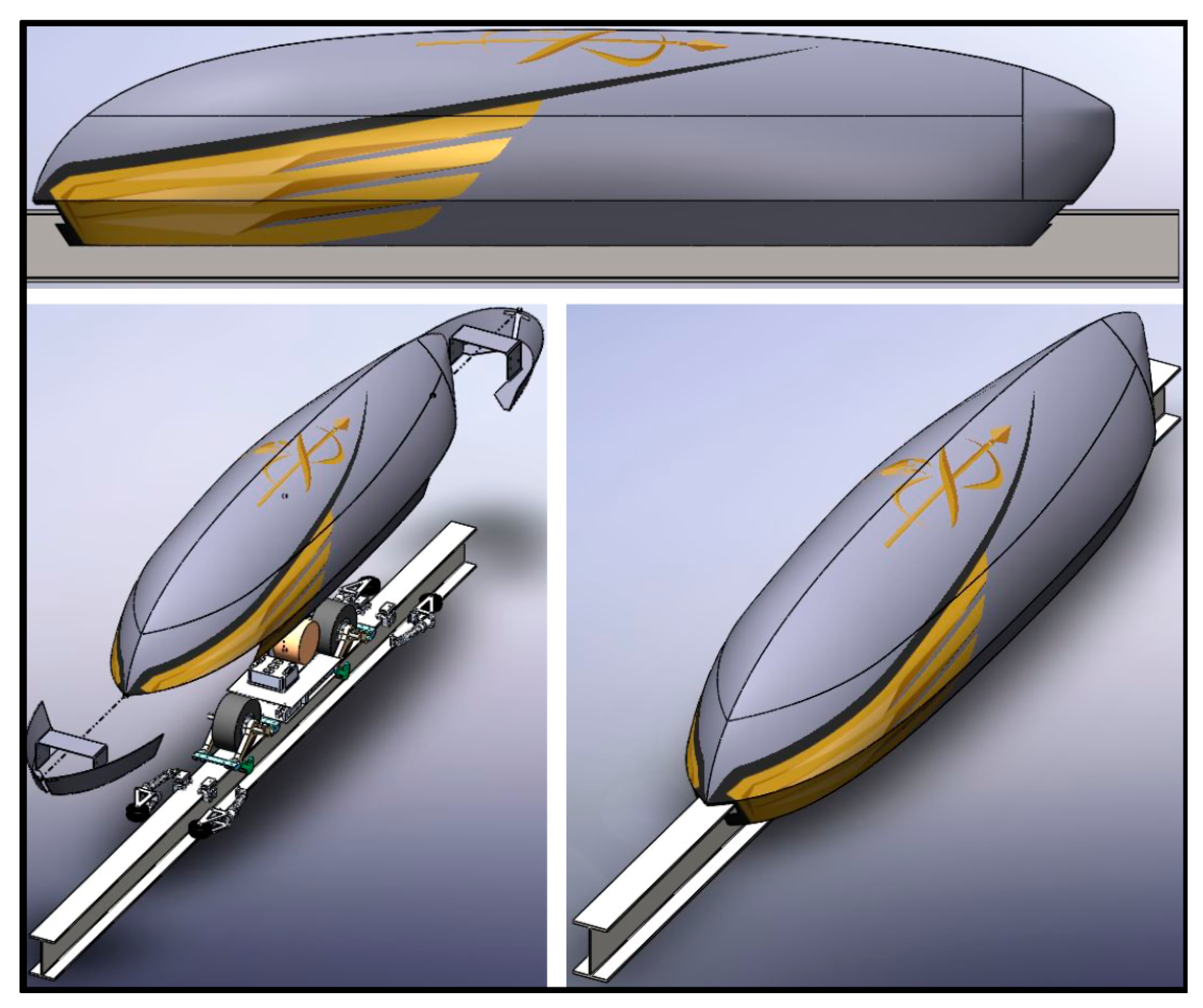
2.4. Phase I Model—Investigation of the Plunger Effect

The model has been made using SolidWorks 2019. For the numerical simulations, ANSYS 19.3 FLUENT (Version 19.3, ANSYS, Canonsburg, PA, USA) has been used. The model for this phase has an overall dimension of 30.5 m length, 4.6 m width, and 3.8 m height. The front of the body resembles a quarter Sears–Haack body [47] (Figure 4), which is defined as a body with the theoretically lowest wave drag in supersonic flow and is modeled by the Prandtl–Glauert equation [48]. The cross-sectional area and the volume of a Sears–Haack body with radius R and length L are given by:

$$S\left(x\right)=\frac{16V}{3L\pi }{[4x\left(1-x\right)]}^{3/2}=\pi R_{max}^2{[4x\left(1-x\right)]}^{3/2}$$

(6)

where R_max represents the maximum radius of the body, x represents the space coordinate, and the V represents the volume. The volume is given by:

$$V=\frac{3{\pi }^2}{16}{R}_{max}^{2}L$$

(7)

The surface area and frontal area of the model were calculated as 530.93 and 14.04 m², respectively. After the models were made, the computational domain was created along with models. Both the models have the same computational domain. The computational domain has been given the shape of the tube in which the pod will be operating. The dimensions of the computational domain are 5.2 m diameter for the upper wall and 4.5 m height of the whole tube while the length is 304.8 m (1000 ft.). The distance between the nose of the pods and the inlet boundary is 152.4 m.

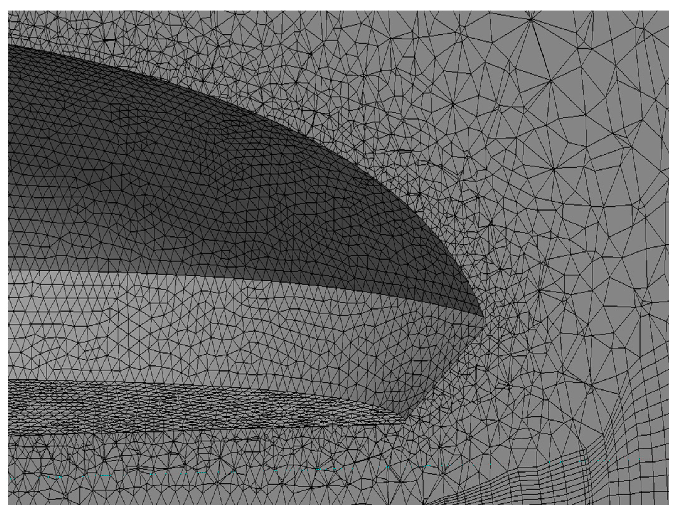
2.5. Mesh Generation and Grid Convergence

The mesh of the computational domain for both models was generated using the wall inflation (y+) method. The y+ wall treatment is the nondimensional distance between the centroid of the cell and the wall. Mathematically, it is defined as:

$$y+=\frac{yu+}{v}$$

(8)

where y+ = nondimensional distance between the wall and the cell centroid.

y = distance between the wall and cell centroid

u* = friction velocity

$v$ = kinematic viscosity

The tetrahedron patch conforming method with quadratic element order was applied for the pod models. The face sizing method was applied to the outer faces of the pod.

Table 1. Results from the grid convergence study performed on the model.

Case	Number of Elements	Drag (n) (Relative Error)	Lift (n) (Relative Error)	Pressure (pa) (Relative Error)	Velocity (m/s) (Relative Error)
Type 1	3,081,385	2793.89 (34.95%)	−185.27 (0%)	227.81 (27.05%)	1374.77 (19.55%)
Type 2	2,236,054	2070.32 (180.95%)	−185.27 (5.29%)	179.31 (15.88%)	1149.87 (14.70%)
Type 3 *	1,601,627	736.9	−195.07	207.8	1319

* Type 3 is used as the reference for this comparison; hence, its relative error is zero.

shows the grid convergence study performed on this model. A type-3 mesh was used for the study and the generated mesh for the model consisted of 1,601,627 elements (Figure 5).

To study the aerodynamic effects of the plunger effect on the Hyperloop pod, we considered four cases for each model. The Mach number corresponding to the Kantrowitz Limit for the model is 0.45 (194.5 m/s). The other speeds considered were 112, 241, and 340 m/s with the Mach numbers being 0.32, 0.7, and 0.9, respectively, to make direct comparison of the results with a previous study [9] possible. The general boundary conditions used for the phase-1 model are shown in

Table 2. Boundary conditions used for the computational models.

Material of the pod	3k Twill weave carbon fiber
Material of the tube	Steel
Material for the fluid	Air
Speeds considered (m/s)	112, 154, 241, 309
Tube pressure (Pa)	25
Tube temperature (°C)	49
Density of fluid (kg/m3)	0.000270
Density of the pod material (kg/m3)	1760

.

No slip boundary conditions were used on the pod surface and the ground floor. The inflow turbulence intensity was set to 5%. All runs have been performed in a transient mode with a time step of 0.1 s, which was considered appropriate to resolve any fluctuations in aerodynamic forces. To solve the coupled equations, the Semi-Implicit Method for Pressure-Linked Equations (SIMPLE) algorithm was used, where several iterations were performed in each time step to ensure convergence. This algorithm in ANSYS FLUENT uses the finite volume method for the spatial discretization. The number of time-steps was limited to 100 with each step of size 0.1 s (for a total time of 10 s). The iterations were allowed to converge and it was observed that convergence occurred between 65 and 80 iterations per time-step (a total of 6500 to 8000 iterations).

2.6. Phase II Model—With Aerofoils to Mitigate the Plunger Effect

The phase-2 model was similar to that of Phase-1 with the addition of aerofoils (Figure 6). The aerofoil chosen was NASA LS (1)-0413 (GA(W)-2) [49]. Data points were used to plot the profile of the foil that enabled us to make its 3D model much more accurate (available in [49]). This aerofoil has a chord length of 1 m, camber length of 0.14 m, and a width of 4.6 m. The computational procedure, meshing, and other characteristics of the analysis remained the same as those in the case of the phase-1 model.

3. Results

The two models are compared based on the results from the computational analysis. Convergence of both cases was achieved between 6000 and 8000 iterations. The subsections below show the comparison of drag and lift coefficients, formation of eddy currents, and the pressure distribution around the two pods.

3.1. Verification and Validation of the Model Used

To study the aerodynamics of the flow around the pod, this study employs the RANS model. RANS is a very popular model for studying complex flow patterns, as evidenced by a number of prior studies [24,25,26,27]. The unsteady RANS model is used to study the turbulent flow. To resolve the smallest turbulent phenomena and fastest fluctuations, Direct Numerical Simulation (DNS) is employed, which uses a very fine mesh and very small time steps. DNS is considered a very reliable method, but computationally intensive [50].

A previous study from Graham [51] explored the effectiveness of various CFD models in simulating the flow around a two-dimensional slot nozzle ejector. In comparison with the experimental data, the SST k-$\omega$ model produced the most accurate results for the mass flow rate and velocity in the turbulent flow. Graham reported that this model provided close-to-experimental results with some small oscillations in the converged solution. He concluded that, among five models considered for analysis, the SST k-$\omega$ model performed best in terms of accuracy, efficiency, and stability of the results.

3.2. Drag Coefficient

It was observed that with the inclusion of the aerofoils, a significantly lower drag coefficient was achieved by the phase 2 pod compared to phase 1 (as shown in Figure 7). The Kantrowitz limit of the phase 2 model was 1.07 times greater than that of phase 1. As the Kantrowitz limit represents the maximum amount of compression a flow experiences before it chokes [9,37], it can be concluded that the Phase-1 model starts choking the airflow a little earlier than Phase-2.

Figure 8 shows the drag coefficients obtained by two similar studies in the literature [9,41] and a comparison of the phase 1 and phase 2 values with those. Please note that a direct comparison of these values is not possible, as all the three studies use different pod profiles, dimensions, and tunnel dimensions. The coefficient of drag in phase 1 and phase 2 pods are significantly higher than those of the other studies due to the constrained space around these pods. In the studies by Opgenoord & Caplan [9] and Oh et al. [41], significantly relaxed constraints are used (more space is available between the pod and the wall of the tunnel) and the pods are significantly smaller in length. In ref. [9], a pod of 2.4 m length with a tunnel pressure of 860 Pa is used. In ref. [41], pods of various lengths are used with their minimum length being 10.75 m. They also showed an increase in the coefficient of drag as the pod length increases, which agrees with these results. Phase 1 and phase 2 pods do show a slight reduction in the coefficient of drag as the Mach number increases—this is primarily due to the design of the aerodynamic profile for the pod. The design for the profile is primarily inspired by the Koenigsegg Regera. Koenigsegg is known to build supercars with a continuous goal of setting and beating records with their precision engineering.

3.3. Lift Coefficient

The lift coefficients for the models are shown in Figure 9. It was observed that the Phase-1 model experienced a negative lift as compared to Phase-2. The results showed that by the addition of the aerofoils, the lift was improved drastically. Optimal lift is required for a Hyperloop pod to move on the maglev rails or air bearings. Hence, the addition of aerofoils is a feasible technique to improve the performance of a Hyperloop pod. None of the previous studies on Hyperloop have evaluated the lift coefficients of their pods.

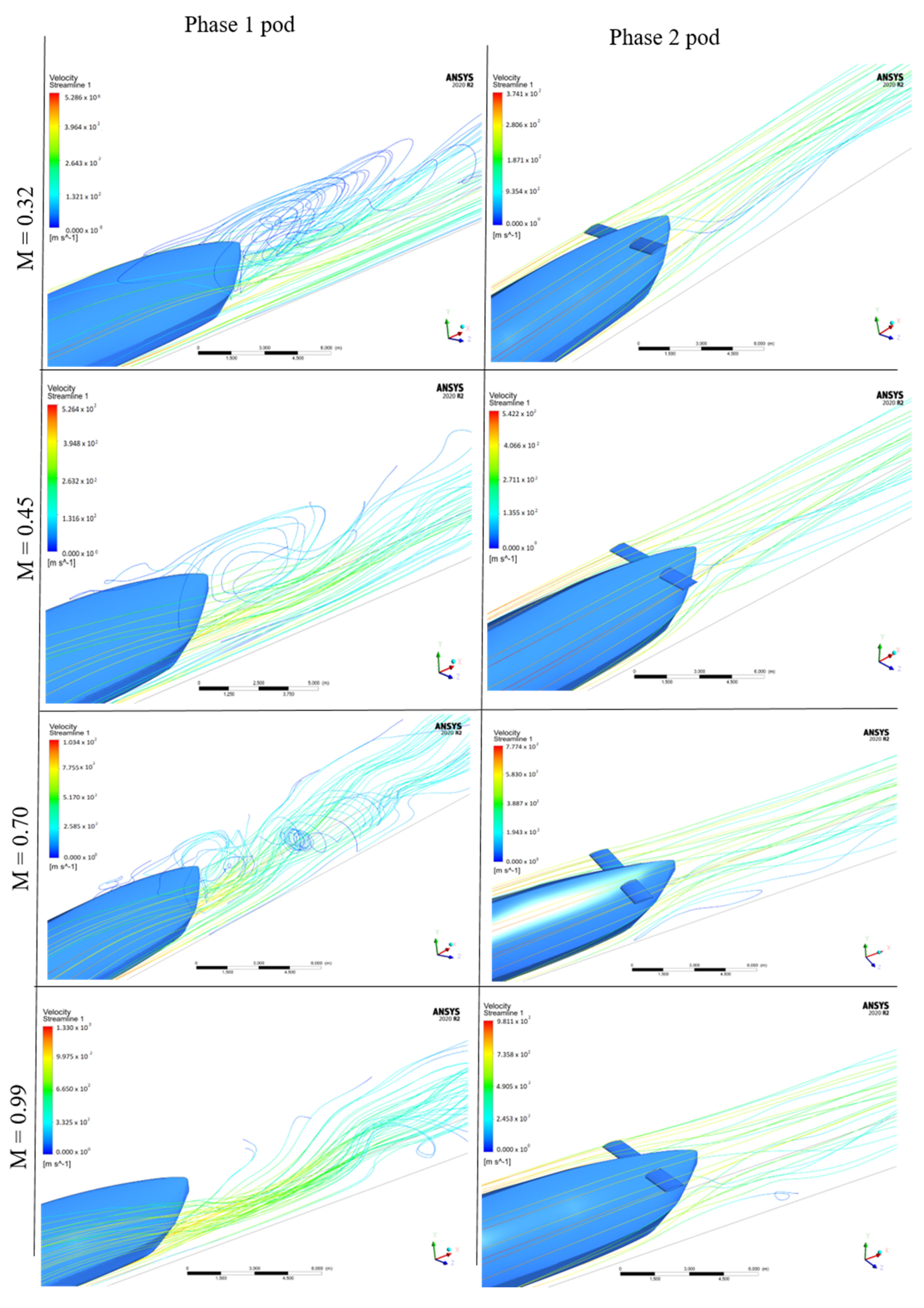
3.4. Formation of Eddy Currents

Next, the velocity stream lines around the pods were studied to understand the formation of eddy currents. Figure 10 shows the stream lines for various Mach numbers. Four different speeds for the pod in the vacuum tube were considered: 112, 154, 241, and 309 m/s. The corresponding Mach numbers for the pod were 0.32, 0.45, 0.70, and 0.9. At M = 0.32, air flow was observed to be unhindered for both models, but Phase-1 had more eddies forming in comparison to Phase-2. Phase-1 was observed to form eddies even before reaching the Kantrowitz limit. After reaching the Kantrowitz limit (at M = 0.45), the air flow got restricted at the top of the pod and the points were formed where the air can pass at very high speeds, primarily due to the very low clearance between the top of the pod and the tunnel’s roof. Other aerodynamic studies on Hyperloop pods [9,41] also showed a very similar behavior of air flow during their analysis. In both these studies, a significant pressure increase is observed at the front of the pod at speeds closer to and above the Kantrowitz limit.

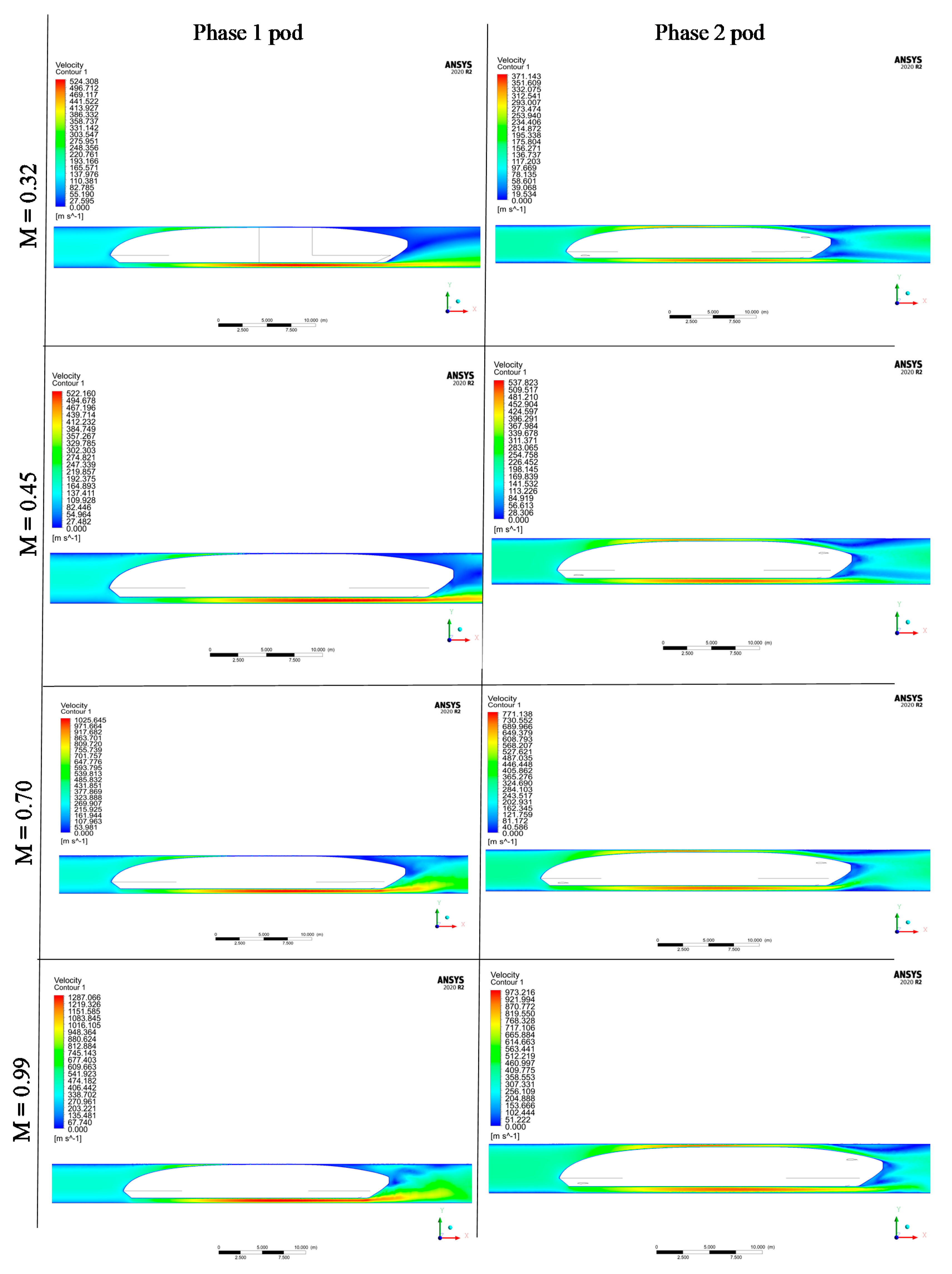
3.5. Velocity Contours

An investigation on the velocity contours around the two pods showed that the Phase-2 pod handled the airflow around it efficiently, as shown in Figure 11. At speeds below the Kantrowitz limit, the air got accumulated at the back of the pod and got diminished as the speed increased. Even after crossing the theoretical Kantrowitz limit, the phase 2 pod performed relatively better, due to the better aerodynamic behavior around it. At lower speeds, the air at the top of the pod was very slow but not completely stagnant. As the speed increased, the air started stagnating at the top, and at 0.9, it was completely stagnant.

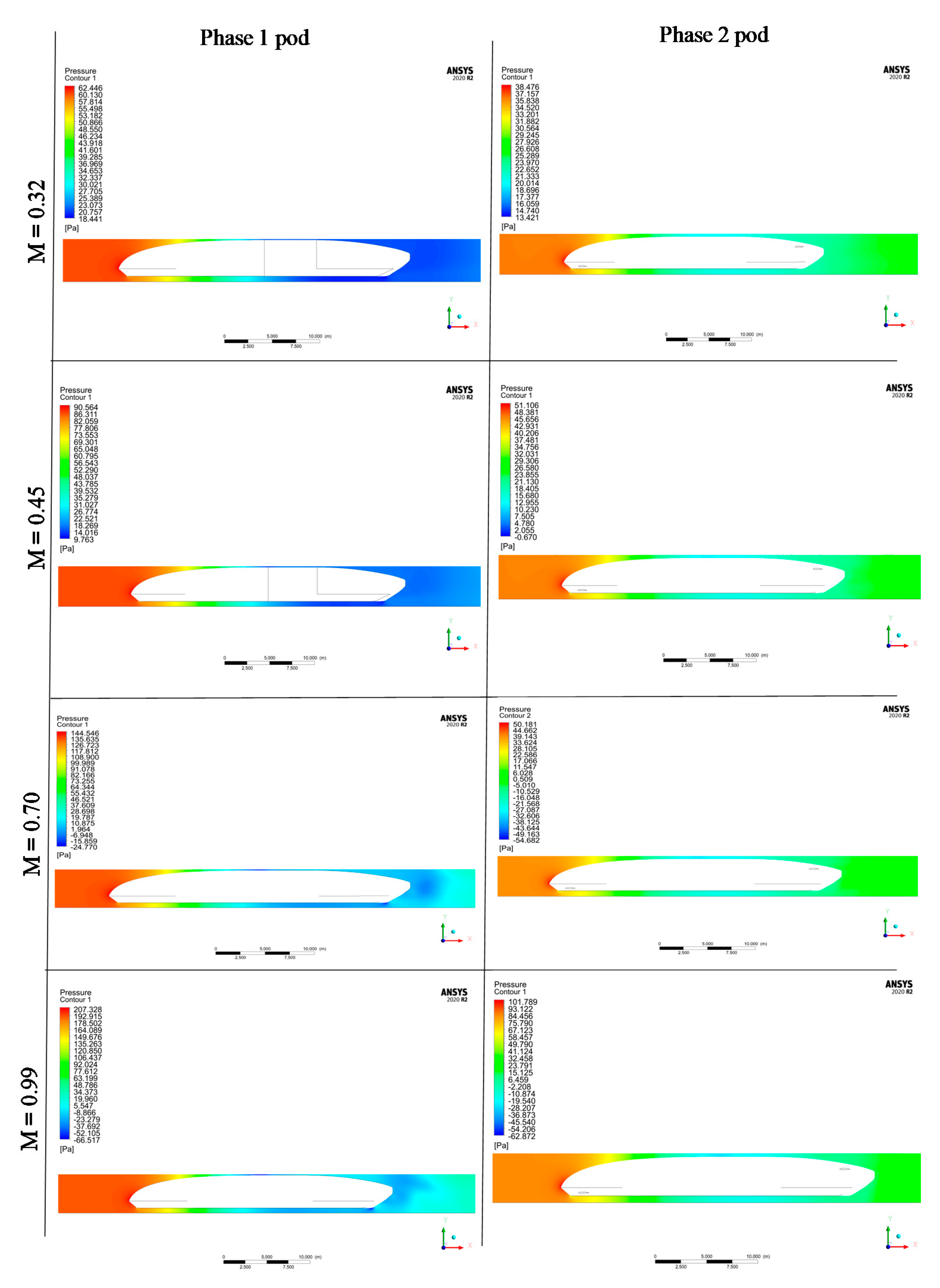
3.6. Pressure Contours

The pressure contours for Phase-1 and Phase-2 models showed that the largest pressure was experienced at the front of the pod where the air made first contact with it (Figure 12). In the Phase-1 model, the pressure was high even at M = 0.32, but this did not create any hindrance to the flow of air. At Mach 0.45 (i.e., the Kantrowitz Limit), the pressure started to build considerably at the largest cross-section, hindering the air flow, and at M = 0.7 and 0.9, a negative pressure was generated, thereby acting as a wall for the air flow to the back of the pod. This demonstrated the presence of the plunger effect when the Hyperloop pod traveled at a very high speed. With the aerofoils in the phase-2 model, the plunger effect was still present, but the pressure buildup in the front of the pod was observed to be significantly smaller.

The pressure contours generated in this analysis are very similar to those from Opgenoord and Caplan [9], and Oh et al. [41]. In both these studies, the researchers have observed the development of high-pressure regions and shocks at the front of the pod, especially at speeds approaching the Kantrowitz limit. A direct comparison of the pressure values is not possible, as the analysis conditions are different in these studies. The pod used by Oh et al. has a cylindrical front-end shape, whereas the one from Opgenoord and Caplan features a blunt-nose shape. The airflow around these two profiles is expected to be significantly different and the pods used in this study feature a more aerodynamically optimized profile. However, the pressure contours follow the same trends in all the three studies.

4. Discussion

4.1. Plunger Effect inside the Vacuum Tube

The results clearly demonstrate the presence of choked flow and the plunger effect at very high speeds at which the Hyperloop is expected to operate. The presence of these effects can be influenced by a number of parameters including the aerodynamic profile of the vehicle, the pressure inside the tube, and the relative size of the pod with respect to the tube. The results on the plunger effect agree with prior computational studies on Hyperloop [9,39,40]. As the plunger effect leads to a significant increase in the drag, solutions to reduce the same needs to be devised to increase the energy efficiency of a Hyperloop pod. Previous studies have investigated the use of a compressor that can suck the air inside the pod and reuse it [9,40] as a potential solution. However, a significant amount of energy needs to be spent to operate the compressor. Another possibility is to use compressors on the tube walls so that air can be pumped outside and transported elsewhere. This can also be a very expensive solution. Other potential solutions include a Drag Reduction System (DRS) [52] or a draught relief shaft [53], as used in other transportation methods.

4.2. Use of Aerofoil Fins on Hyperloop Pods

In this study, we explored the use of aerofoil-shaped fins attached to the aeroshell of a Hyperloop pod as a potential method to reduce the plunger effect and thereby reduce the drag. It is observed that the presence of aerofoil fins does help in the reduction of the drag coefficient at all speeds. While the original aeroshell design creates a negative lift during the analysis, the presence of aerofoils helps in generating a positive lift. This can be very helpful in Hyperloop systems that depend on levitation-based propulsion mechanisms such as magnetic levitation and air bearings. Further, the presence of aerofoils helps in reducing the eddy formation and pressure build-up at the front of the pod.

4.3. Limitations of the Study

In this paper, a CFD analysis of the Hyperloop pod is used for demonstrating the plunger effect and investigating its mitigation using aerofoil-shaped fins on the body of the pod. No experimental data are available to compare these results with, and hence, the true validation of these results is not possible. In the current study, verification and validation is performed by comparing the results with those from a limited number of previous similar studies in the literature. Additional studies and experimental investigation using a full-scale pod and a wind tunnel are currently being planned as future work.

5. Conclusions

The turbulent flow of air inside a tube in which a Hyperloop pod is operating over realistic conditions has been numerically simulated by solving unsteady three-dimensional RANS equations. The computed outcomes for aerodynamic coefficients using an SST k-ω turbulence model provides us with the visualization on the velocity and pressure contours as the pod moves inside a steel tube at high Mach speeds. It also shows that the unsteady CFD-RANS method can generate important aerodynamic results when combined with an appropriate turbulence model. The results and data obtained show that the use of aerofoils can help mitigate the effects of the plunger effect. The velocity contours show that the air flows through the phase-2 pod in comparison with the phase-1 pod in all cases. Based on the streamlines, it is observed that there are no eddies for the phase-2 model for Mach numbers 0.32 and 0.45. Eddy formation starts at Mach numbers of 0.7 and 0.9, but those can be considered negligible. The phase-1 model with no aerofoils creates a number of eddies even for speeds less than the Kantrowitz limit. The pressure comparison around the pod in phase-1 is much more abrupt with negative pressure being generated as the air progresses through the pod in the tube as compared to phase-2 where the pressure change along the pod is steady even in a turbulent flow. The maximum pressure in phase-2 is also less than that in phase-1. This leads to less drag and more lift for phase-2. Overall, phase-2 has a much better aerodynamic performance compared to phase-1. This demonstrates that the addition of aerofoil-shaped fins to the aeroshell of a Hyperloop pod is a feasible technique to reduce the drag and save the cost of operation of the system.

References

1. Sakowski, M. The Next Contender in High Speed Transport Elon Musks Hyperloop. J. Undergrad. Res. Univ. Ill. Chic. 2016, 9, 47–49. [Google Scholar] [CrossRef]
2. Clary, D.A. Rocket Man: Robert H. Goddard and the Birth of the Space Age; Hachette: London, UK, 2003. [Google Scholar]
3. Goddard, E.C. Vacuum Tube Transportation System. U.S. Patent No. 2,511,979, 20 June 1950. [Google Scholar]
4. Yaghoubi, H. The Most Important Maglev Applications. J. Eng. 2013, 2013, 537986. [Google Scholar] [CrossRef] [Green Version]
5. Powell, J.; Danby, G.T.; Jordan, J.C. The Fight for Maglev: Making America the World Leader in 21st Century Transport; CreateSpace: Scotts Valley, CA, USA, 2012. [Google Scholar]
6. van Goeverden, K.; Milakis, D.; Janic, M.; Konings, R. Analysis and modelling of performances of the HL (Hyperloop) transport system. Eur. Transp. Res. Rev. 2018, 10, 41. [Google Scholar] [CrossRef]
7. Musk, E. Hyperloop Alpha; Spacex: Hawthorne, CA, USA, 2013. [Google Scholar]
8. Chaidez, E.; Bhattacharyya, S.P.; Karpetis, A.N. Levitation Methods for Use in the Hyperloop High-Speed Transportation System. Energies 2019, 12, 4190. [Google Scholar] [CrossRef] [Green Version]
9. Opgenoord, M.M.; Caplan, P.C. Aerodynamic design of the Hyperloop concept. AIAA J. 2018, 56, 4261–4270. [Google Scholar] [CrossRef]
10. Pan, S.; Fan, L.; Liu, J.; Xie, J.; Sun, Y.; Cui, N.; Zhang, L.; Zheng, B. A review of the piston effect in subway stations. Adv. Mech. Eng. 2013, 5, 950205. [Google Scholar] [CrossRef]
11. Bonnett, C.F. Practical Railway Engineering; Imperial College Press: London, UK, 2005. [Google Scholar]
12. Takayama, K.; Sasoh, A.; Onodera, O.; Kaneko, R.; Matsui, Y. Experimental investigation on tunnel sonic boom. Shock Waves 1995, 5, 127–138. [Google Scholar] [CrossRef]
13. Auvity, B.; Bellenoue, M.; Kageyama, T. Experimental study of the unsteady aerodynamic field outside a tunnel during a train entry. Exp. Fluids 2001, 30, 221–228. [Google Scholar] [CrossRef]
14. Baker, C. Train aerodynamic forces and moments from moving model experiments. J. Wind Eng. Ind. Aerodyn. 1986, 24, 227–251. [Google Scholar] [CrossRef]
15. Baker, C.; Brockie, N. Wind tunnel tests to obtain train aerodynamic drag coefficients: Reynolds number and ground simulation effects. J. Wind Eng. Ind. Aerodyn. 1991, 38, 23–28. [Google Scholar] [CrossRef]
16. Brockie, N.; Baker, C. The aerodynamic drag of high speed trains. J. Wind Eng. Ind. Aerodyn. 1990, 34, 273–290. [Google Scholar] [CrossRef]
17. Watkins, S.; Saunders, J.; Kumar, H. Aerodynamic drag reduction of goods trains. J. Wind Eng. Ind. Aerodyn. 1992, 40, 147–178. [Google Scholar] [CrossRef]
18. Xia, C.; Shan, X.; Yang, Z. Wall interference effect on the aerodynamics of a high-speed train. Procedia Eng. 2015, 126, 527–531. [Google Scholar] [CrossRef] [Green Version]
19. Lee, Y.; Kim, K.H.; Rho, J.H.; Kwon, H.B. Investigation on aerodynamic drag of Korean high speed train (HEMU-430X) due to roof apparatus for electrical device. J. Mech. Sci. Technol. 2016, 30, 1611–1616. [Google Scholar] [CrossRef]
20. Li, Z.-w.; Yang, M.-z.; Huang, S.; Liang, X. A new method to measure the aerodynamic drag of high-speed trains passing through tunnels. J. Wind Eng. Ind. Aerodyn. 2017, 171, 110–120. [Google Scholar] [CrossRef]
21. Yang, Q.-S.; Song, J.-H.; Yang, G.-W. A moving model rig with a scale ratio of 1/8 for high speed train aerodynamics. J. Wind Eng. Ind. Aerodyn. 2016, 152, 50–58. [Google Scholar] [CrossRef] [Green Version]
22. Catanzaro, C.; Cheli, F.; Rocchi, D.; Schito, P.; Tomasini, G. High-speed train crosswind analysis: CFD study and validation with wind-tunnel tests. In Proceedings of the International Conference on the Aerodynamics of Heavy Vehicles, Potsdam, Germany, 12–17 September 2010; pp. 99–112. [Google Scholar]
23. Paradot, N.; Talotte, C.; Garem, H.; Delville, J.; Bonnet, J.-P. A comparison of the numerical simulation and experimental investigation of the flow around a high speed train. In Proceedings of the Fluids Engineering Division Summer Meeting, Montreal, QC, Canada, 14–18 July 2002; pp. 1055–1060. [Google Scholar]
24. Shin, C.-H.; Park, W.-G. Numerical study of flow characteristics of the high speed train entering into a tunnel. Mech. Res. Commun. 2003, 30, 287–296. [Google Scholar] [CrossRef]
25. Li, X.-H.; Deng, J.; Chen, D.-W.; Xie, F.-F.; Zheng, Y. Unsteady simulation for a high-speed train entering a tunnel. J. Zhejiang Univ. Sci. A 2011, 12, 957–963. [Google Scholar] [CrossRef]
26. Wang, D.; Li, W.; Zhao, W.; Han, H. Aerodynamic Numerical Simulation for EMU Passing Each Other in Tunnel. In Proceedings of the 1st International Workshop on High-Speed and Intercity Railways, Hong Kong, 19–22 July 2011; pp. 143–153. [Google Scholar]
27. Chu, C.-R.; Chien, S.-Y.; Wang, C.-Y.; Wu, T.-R. Numerical simulation of two trains intersecting in a tunnel. Tunn. Undergr. Space Technol. 2014, 42, 161–174. [Google Scholar] [CrossRef]
28. Smagorinsky, J. General circulation experiments with the primitive equations: I. The basic experiment. Mon. Weather Rev. 1963, 91, 99–164. [Google Scholar] [CrossRef]
29. Krajnović, S.; Ringqvist, P.; Nakade, K.; Basara, B. Large eddy simulation of the flow around a simplified train moving through a crosswind flow. J. Wind Eng. Ind. Aerodyn. 2012, 110, 86–99. [Google Scholar] [CrossRef]
30. Zhuang, Y.; Lu, X. Numerical investigation on the aerodynamics of a simplified high-speed train under crosswinds. Theor. Appl. Mech. Lett. 2015, 5, 181–186. [Google Scholar] [CrossRef] [Green Version]
31. Khayrullina, A.; Blocken, B.; Janssen, W.; Straathof, J. CFD simulation of train aerodynamics: Train-induced wind conditions at an underground railroad passenger platform. J. Wind Eng. Ind. Aerodyn. 2015, 139, 100–110. [Google Scholar] [CrossRef]
32. García, J.; Muñoz-Paniagua, J.; Crespo, A. Numerical study of the aerodynamics of a full scale train under turbulent wind conditions, including surface roughness effects. J. Fluids Struct. 2017, 74, 1–18. [Google Scholar] [CrossRef]
33. Muld, T.W.; Efraimsson, G.; Henningson, D.S. Flow structures around a high-speed train extracted using proper orthogonal decomposition and dynamic mode decomposition. Comput. Fluids 2012, 57, 87–97. [Google Scholar] [CrossRef]
34. Xia, C.; Wang, H.; Shan, X.; Yang, Z.; Li, Q. Effects of ground configurations on the slipstream and near wake of a high-speed train. J. Wind Eng. Ind. Aerodyn. 2017, 168, 177–189. [Google Scholar] [CrossRef]
35. Wang, S.; Bell, J.R.; Burton, D.; Herbst, A.H.; Sheridan, J.; Thompson, M.C. The performance of different turbulence models (URANS, SAS and DES) for predicting high-speed train slipstream. J. Wind Eng. Ind. Aerodyn. 2017, 165, 46–57. [Google Scholar] [CrossRef]
36. Mei, Y.; Zhou, C. The One-Dimensional Unsteady Flow Prediction Method and Applications on the Pressure Waves Generated by High-Speed Trains Passing through a Tunnel. In Proceedings of the 1st International Workshop on High-Speed and Intercity Railways, Hong Kong, 19–22 July 2011; pp. 397–405. [Google Scholar]
37. Kantrowitz, A.; Donaldson, C. Preliminary investigations of supersonic diffuser, duP. Naca WR L 1945, 713, 2–11. [Google Scholar]
38. Chin, J.C.; Gray, J.S. Open-source conceptual sizing models for the hyperloop passenger pod. In Proceedings of the 56th AIAA/ASCE/AHS/ASC Structures, Structural Dynamics, and Materials Conference, Kissimmee, FL, USA, 5–9 January 2015; p. 1587. [Google Scholar]
39. Braun, J.; Sousa, J.; Pekardan, C. Aerodynamic design and analysis of the hyperloop. AIAA J. 2017, 55, 4053–4060. [Google Scholar] [CrossRef]
40. Yang, Y.; Wang, H.; Benedict, M.; Coleman, D. Aerodynamic simulation of high-speed capsule in the Hyperloop system. In Proceedings of the 35th AIAA Applied Aerodynamics Conference, Denver, CO, USA, 5–9 June 2017; p. 3741. [Google Scholar]
41. Oh, J.-S.; Kang, T.; Ham, S.; Lee, K.-S.; Jang, Y.-J.; Ryou, H.-S.; Ryu, J. Numerical analysis of aerodynamic characteristics of hyperloop system. Energies 2019, 12, 518. [Google Scholar] [CrossRef] [Green Version]
42. Biadgo, A.M.; Simonović, A.; Svorcan, J.; Stupar, S. Aerodynamic characteristics of high speed train under turbulent cross winds: A numerical investigation using unsteady-RANS method. Fme Trans. 2014, 42, 10–18. [Google Scholar] [CrossRef] [Green Version]
43. Schlichting, H.; Gersten, K. Boundary-Layer Theory; Springer: Berlin/Heidelberg, Germany, 2016. [Google Scholar]
44. Wilcox, D.C. Turbulence Modeling for CFD; DCW Industries: La Cañada, CA, USA, 1998; Volume 2. [Google Scholar]
45. Menter, F.R. Two-equation eddy-viscosity turbulence models for engineering applications. AIAA J. 1994, 32, 1598–1605. [Google Scholar] [CrossRef] [Green Version]
46. Taylor, R.E. Specific Heat of Carbon/Carbon Composites; Airforce Office of Scientific Research: West Lafayette, IN, USA, 1981. [Google Scholar]
47. Palaniappan, K.; Jameson, A. Bodies having Minimum Pressure Drag in Supersonic Flow—Investigating Nonlinear Effects. J. Aircr. 2010, 47, 1451–1454. [Google Scholar] [CrossRef] [Green Version]
48. Nathman, J. The Solution of the Prandtl-Glauert Equation around Non-slender Bodies. Anal. Method Rep. 1987, 8, 7–15. [Google Scholar]
49. Nasa/Langley. LS(1)-0413 (GA(W)-2) Airfoil. Available online: https://m-selig.ae.illinois.edu/ads/coord/ls413.dat (accessed on 27 October 2020).
50. Moin, P.; Mahesh, K. Direct numerical simulation: A tool in turbulence research. Annu. Rev. Fluid Mech. 1998, 30, 539–578. [Google Scholar] [CrossRef] [Green Version]
51. Graham, C. Evaluation of the Performance of Various Turbulence Models for Accurate Numerical Simulation of a 2D Slot Nozzle Ejector; Washington University at St. Louis: St. Louis, MO, USA, 2014. [Google Scholar]
52. Rinard, G. Vehicle Drag Reduction System. U.S. Patent No. 5,280,990, 8 July 2014. [Google Scholar]
53. Lin, C.J.; Chuah, Y.K.; Liu, C.W. A study on underground tunnel ventilation for piston effects influenced by draught relief shaft in subway system. Appl. Therm. Eng. 2008, 28, 372–379. [Google Scholar] [CrossRef]
Figure 1. Pressure build-up (piston effect) in front of high-speed vehicles in tunnels.
Energies 14 00464 g001
Figure 2. The modular aeroshell design of the Spartan Hyperloop competition team. The design uses a modular concept to account for the design for manufacturability and assembly considerations.
Energies 14 00464 g002
Figure 3. The overall dimensions of the Hyperloop pod used in this study. All lengths are in m.
Energies 14 00464 g003
Figure 4. Isometric view of the Phase-1 model.
Energies 14 00464 g004
Figure 5. Cross-sectional mesh of the model.
Energies 14 00464 g005
Figure 6. Isometric view of Phase-2 model.
Energies 14 00464 g006
Figure 7. Drag coefficients for the pod models.
Energies 14 00464 g007
Figure 8. Drag coefficients for the pod models.
Energies 14 00464 g008
Figure 9. Lift coefficients for the pod models.
Energies 14 00464 g009
Figure 10. Comparison of the stream lines around the two pods. It was observed that the phase 2 pod led to fewer eddy currents compared to the phase 1 pod.
Energies 14 00464 g010
Figure 11. A comparison of the velocity contours around the two pods.
Energies 14 00464 g011
Figure 12. A comparison of the pressure contours around the two pods. The pressure in all the cases is maximum at the front of the pod, especially around the nose.
Energies 14 00464 g012