
An Open-Source Monte Carlo Ray-Tracing Simulation Tool for Luminescent Solar Concentrators with Validation Studies Employing Scattering Phosphor Films

Abstract

1. Background and Motivation
2. Existing MC Models in the Literature
3. General Description of Classes Used within the MC Model to Establish LSC Components
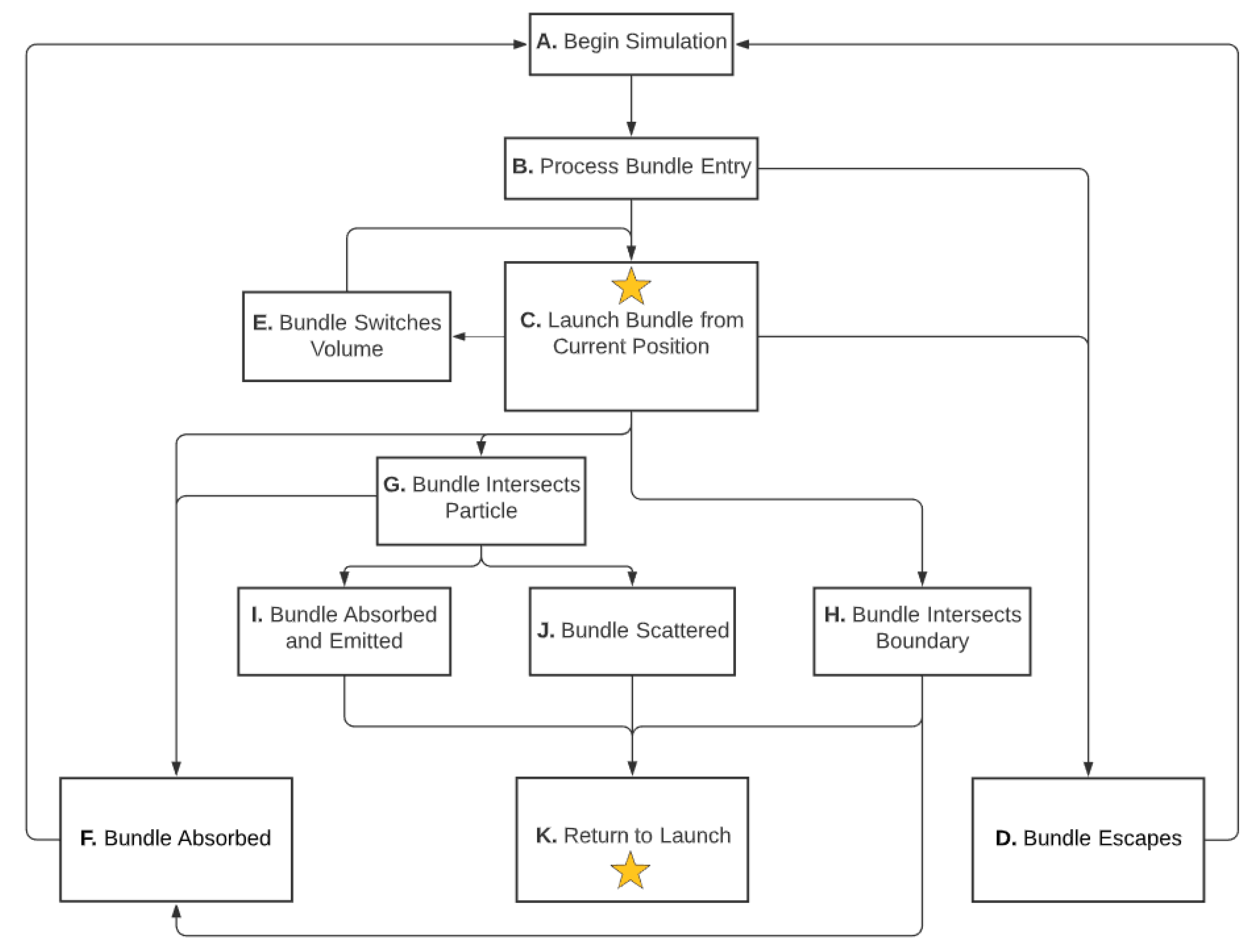
- Bundle: A bundle object represents a “packet of photons”. It tracks the characteristics and position of the packet of photons as it moves through various volume objects and interacts with boundary and particle objects. Bundles are tracked in lieu of photons, as they have constant energy and can be easily sampled from irradiance spectra.
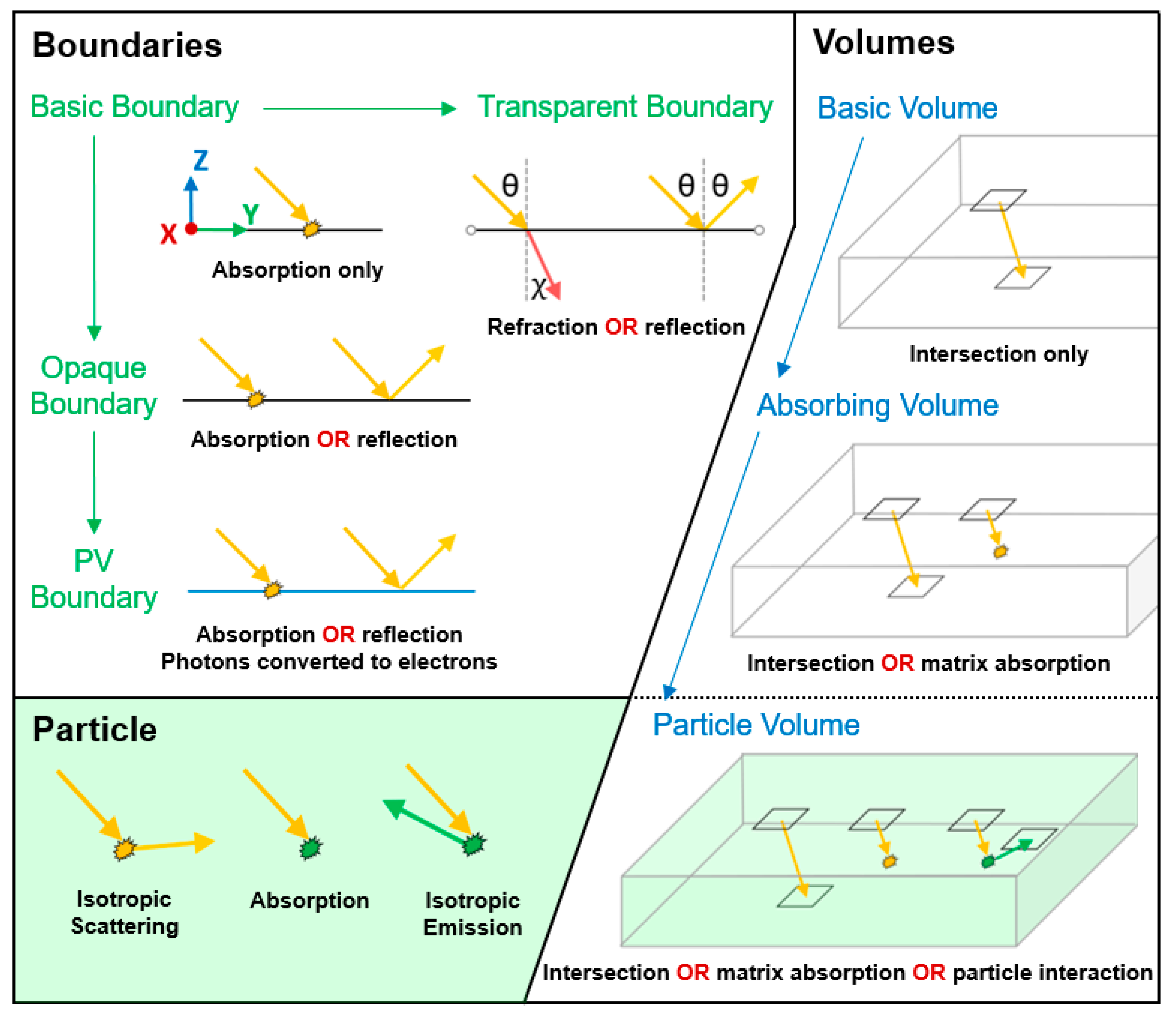
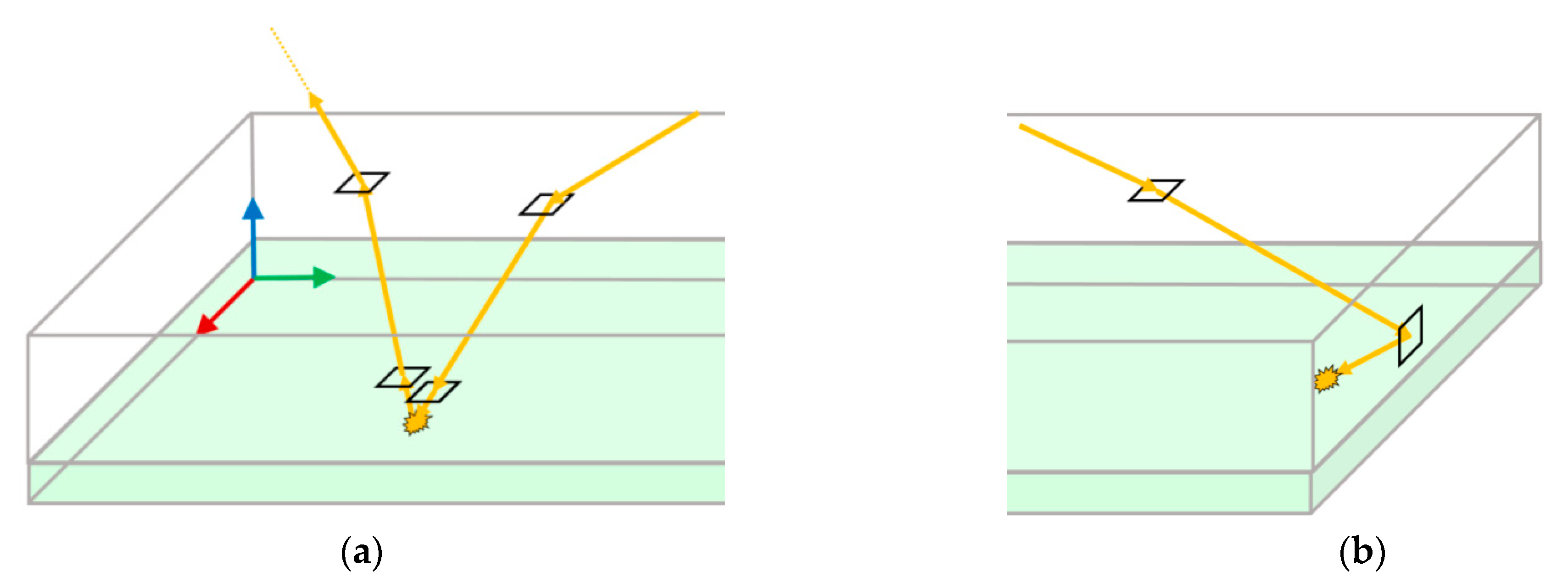
- Volume: A volume object is a bounding region that consists of a particular material, providing the medium that a bundle will traverse through. Each volume has corresponding boundary objects, representing the facets of a particular volume. There are three types of volumes: basic volumes, absorbing volumes, and particle volumes. Bundles may be absorbed as they move throughout volume objects. Absorbing volumes inherit all functionality of basic volumes, and particle volumes inherit all functionality of absorbing volumes. Additionally, as bundles move through particle volumes, they may interact with a particle object.
- Boundary: A boundary object contains the properties inherent to a facet. At a boundary, a bundle can be reflected, transmitted, or absorbed with varying probability, depending on the characteristics specific to that boundary object. There are four types of boundaries: basic boundaries, transparent boundaries, opaque boundaries, and PV boundaries. Opaque and transparent boundaries inherit all functionality from the basic boundary class. PV boundaries inherit all functionality from the opaque boundary class.
- Particle: A particle object represents a scattering and/or absorbing and emitting element and tracks the characteristics of that element. A single particle object represents the many particles dispersed throughout a particular volume. In other words, a particle object is assigned to a particle volume to process light interaction with luminescent particles. For the LSCs modeled here, these are phosphor particles.
3.1. Bundle
3.2. Volumes
3.2.1. Basic Volume
3.2.2. Absorbing Volume
3.2.3. Particle Volume
3.3. Boundaries
3.3.1. Basic Boundary
3.3.2. Transparent Boundary
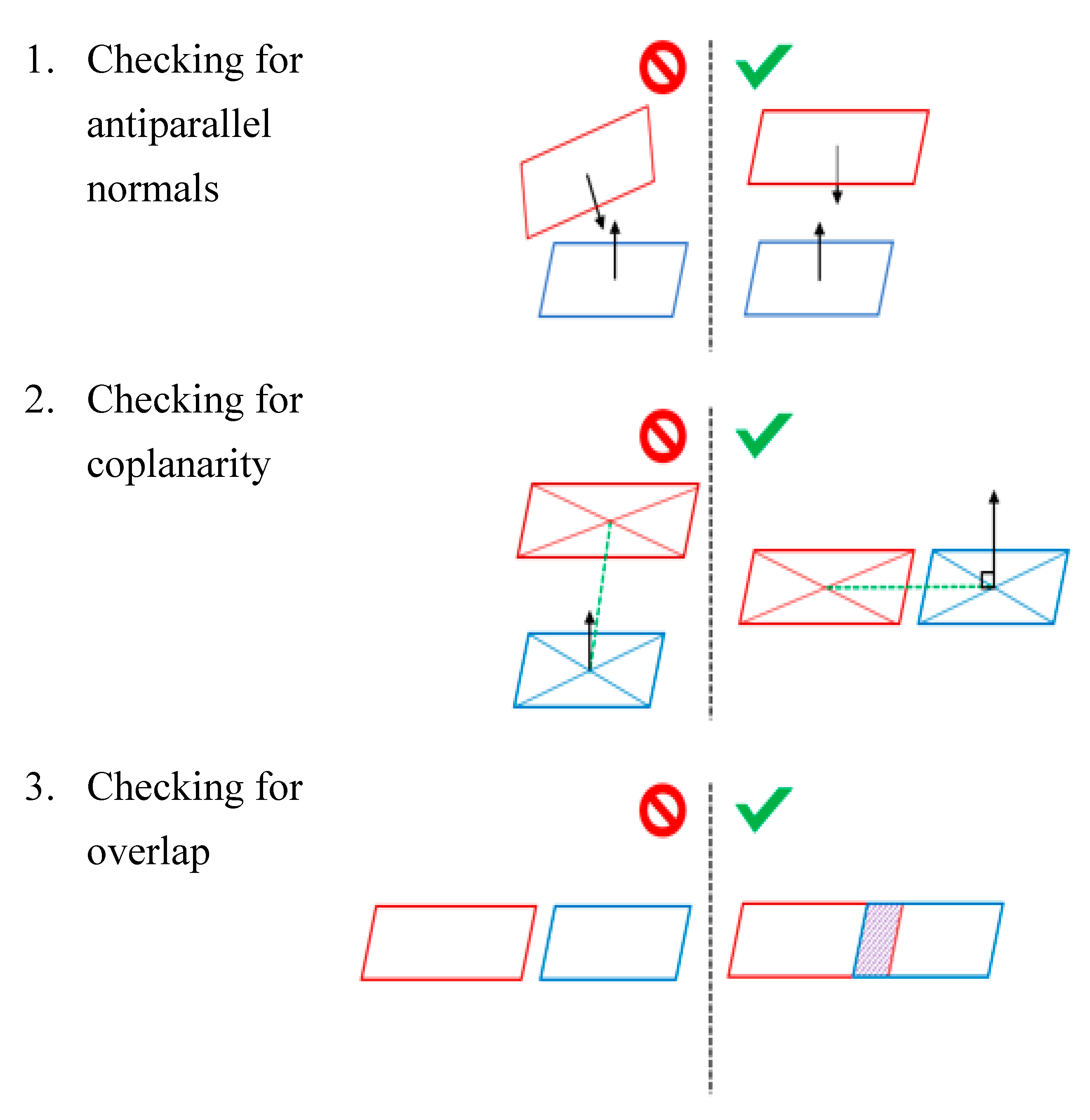
- Checking for antiparallel normals: Normals face inward toward the center of a volume; therefore, transparent boundaries sharing an interface must have normal vectors pointing in exactly opposite directions.
- Checking for coplanarity: The boundaries sharing an interface must fall along the same plane. The line falling between the centers of each boundary must therefore form a right angle with each normal vector.
- Checking for overlap: Now that it is known that boundaries face opposite directions and are coplanar, the area of intersection can be found easily in 2D using the Shapely library. If there is no area of intersection, the boundary is not an interface.
3.3.3. Opaque Boundary
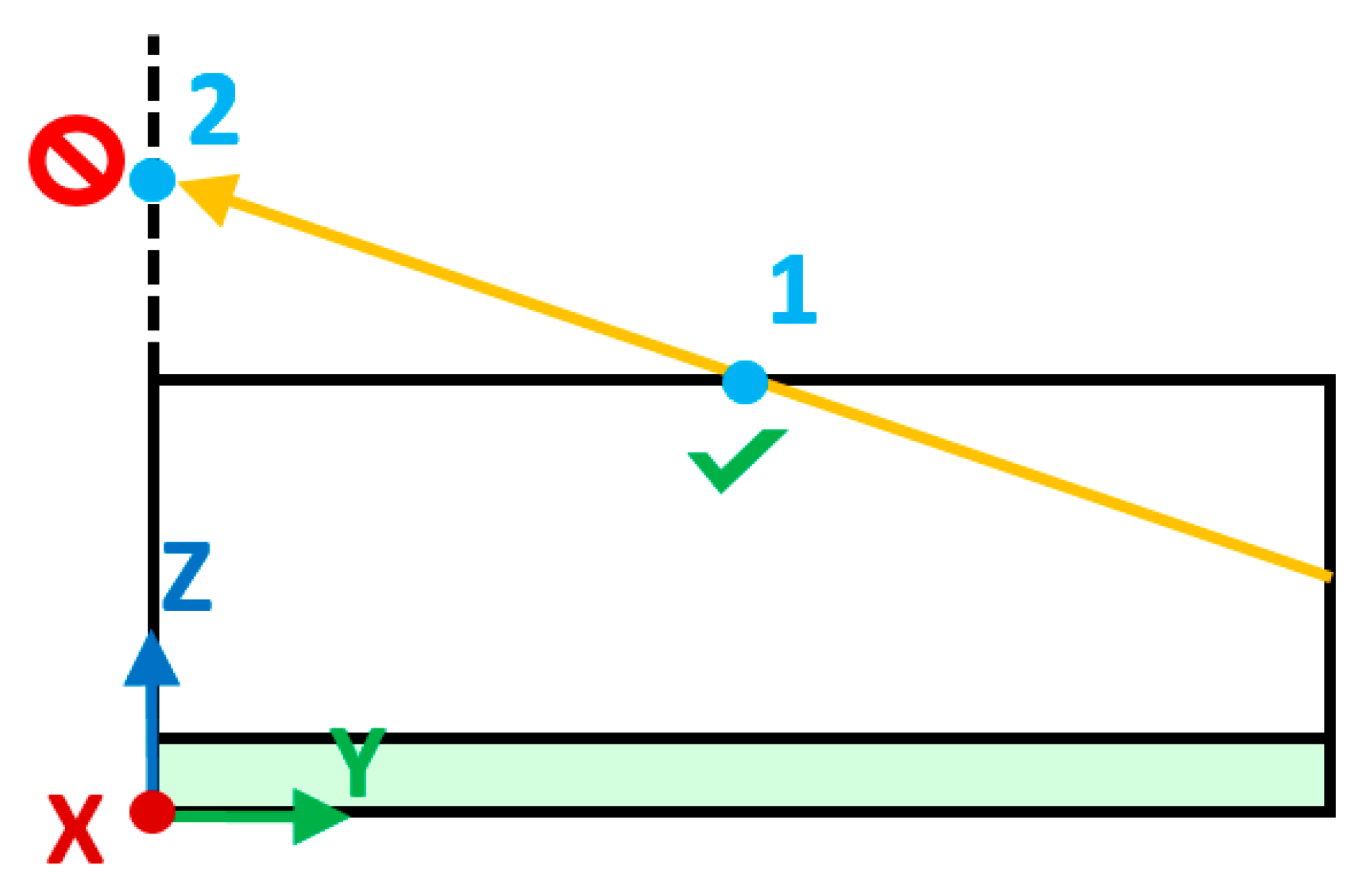
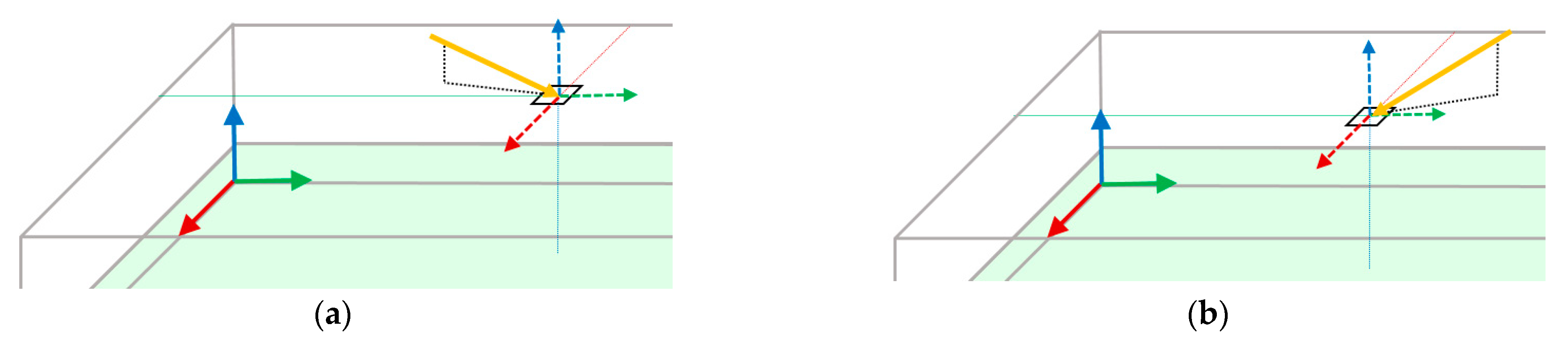
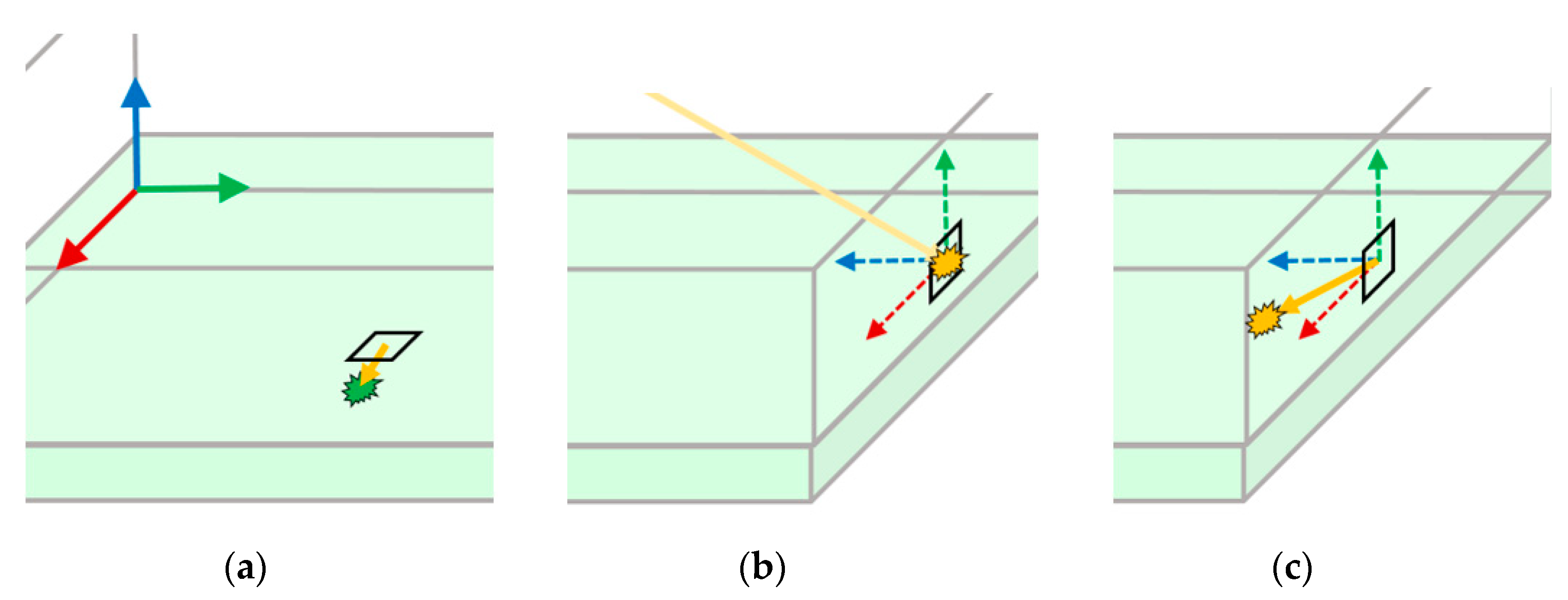
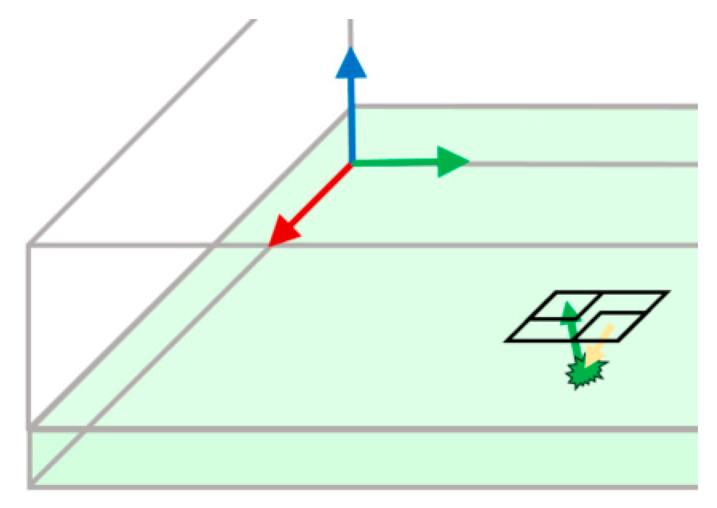
- First, the bundle’s global coordinates are converted from spherical coordinates (, ) to Cartesian coordinates (, , ). Equations (12)–(14) show this conversion.where (, , ) and (, ) are the global coordinates of the incident light vector on a boundary.
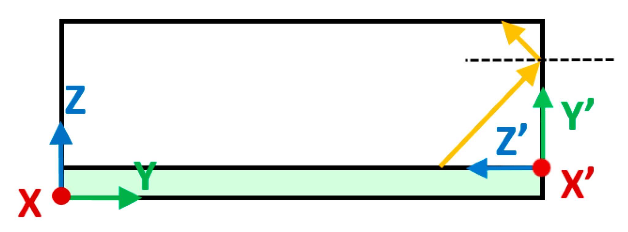
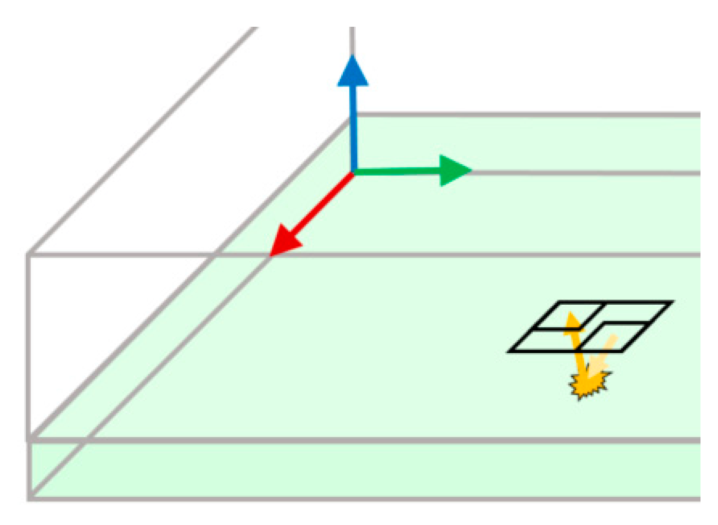
- The (, , ) coordinates are then rotated into the local coordinates (, , ) of the boundary. For the example shown in Figure 8, this is a 90° rotation over the x-axis. Equation (15) depicts the rotational matrix, , employed to rotate over the x-axis, and Equation (16) shows the transformation of the incident light vector from global to local coordinates.
- 3.
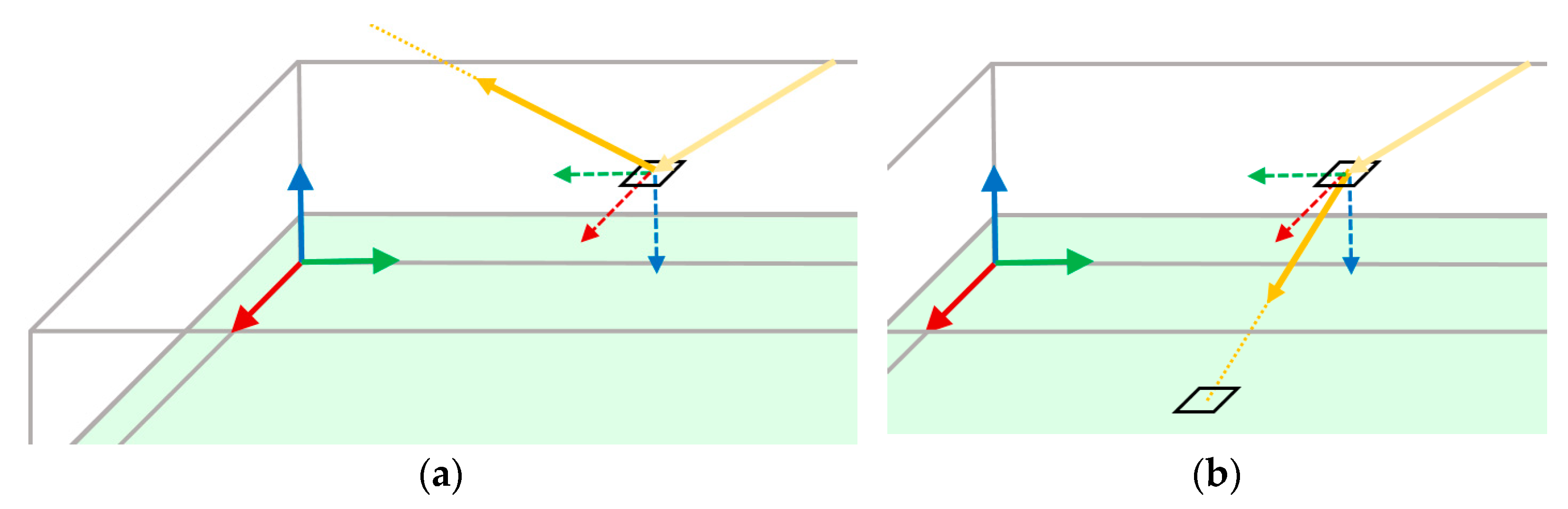
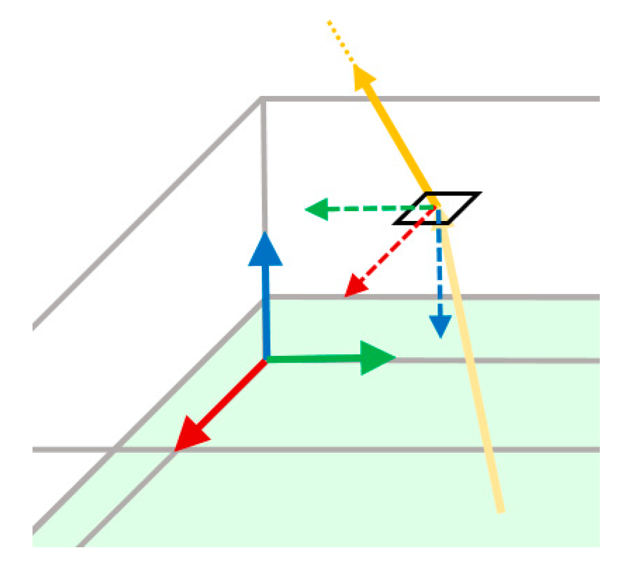
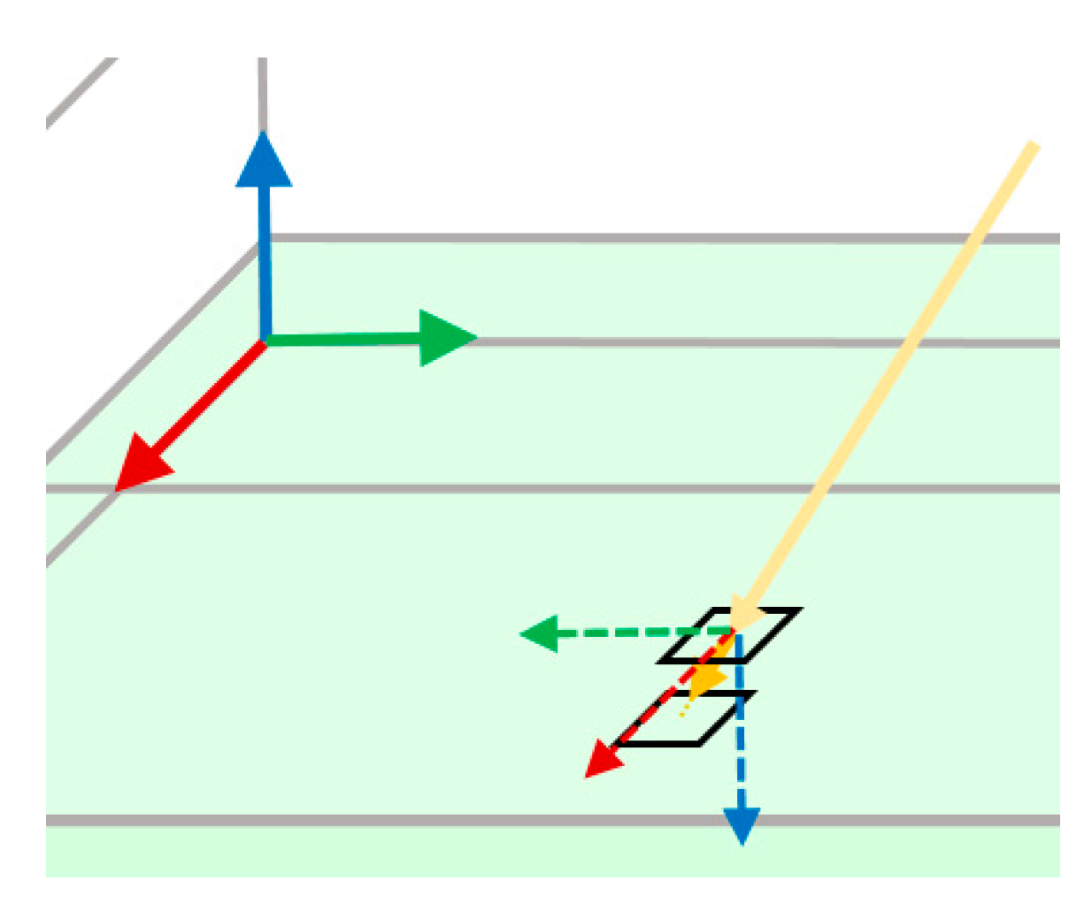
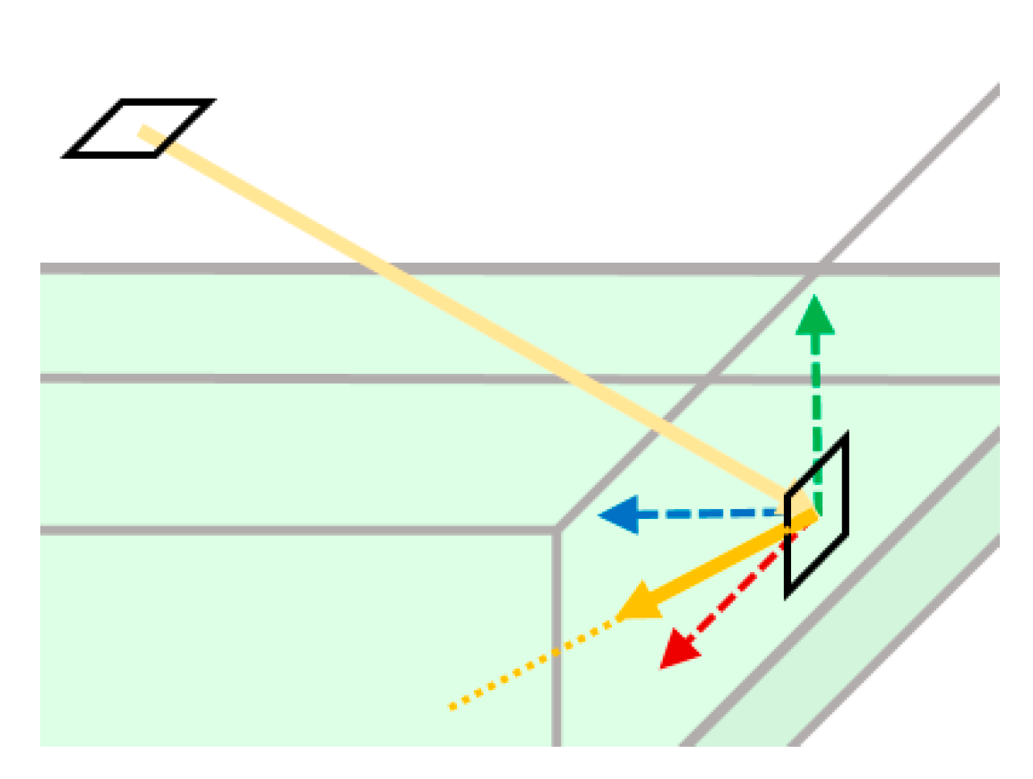
- The incident light vector associated with the bundle is then processed in local coordinates according to a boundary’s assigned properties. For example, to model specular reflection at a mirrored boundary (Figure 8), the incident light vector expressed in local coordinates is rotated by 180° over the -axis, and the direction of the vector is multiplied by -1. Equation (17) shows the rotational matrix, , employed to rotate over the -axis, and Equation (18) shows the transformation employed to process specular reflection.
- 4.
- With a new vector direction determined in local coordinates, the vector is rotated back into the global coordinate system (x, y, z) to prepare to launch to the next boundary. Equation (21) depicts this transformation.
- 5.
- In the final step, the Cartesian coordinates (, , ) of the light vector associated with the bundle are converted back into spherical coordinates (, ) using:where (, ) are the global coordinates of the reflected vector. This vector is now ready for use in intersection calculations.
3.3.4. PV Boundary
3.4. Particle
4. Model Implementation Using Pre-Defined Objects Representing LSC Components
5. MC Model Validation
5.1. Object Attributes Used in Validation Studies
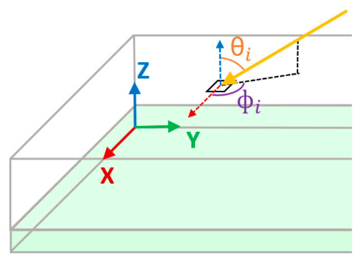
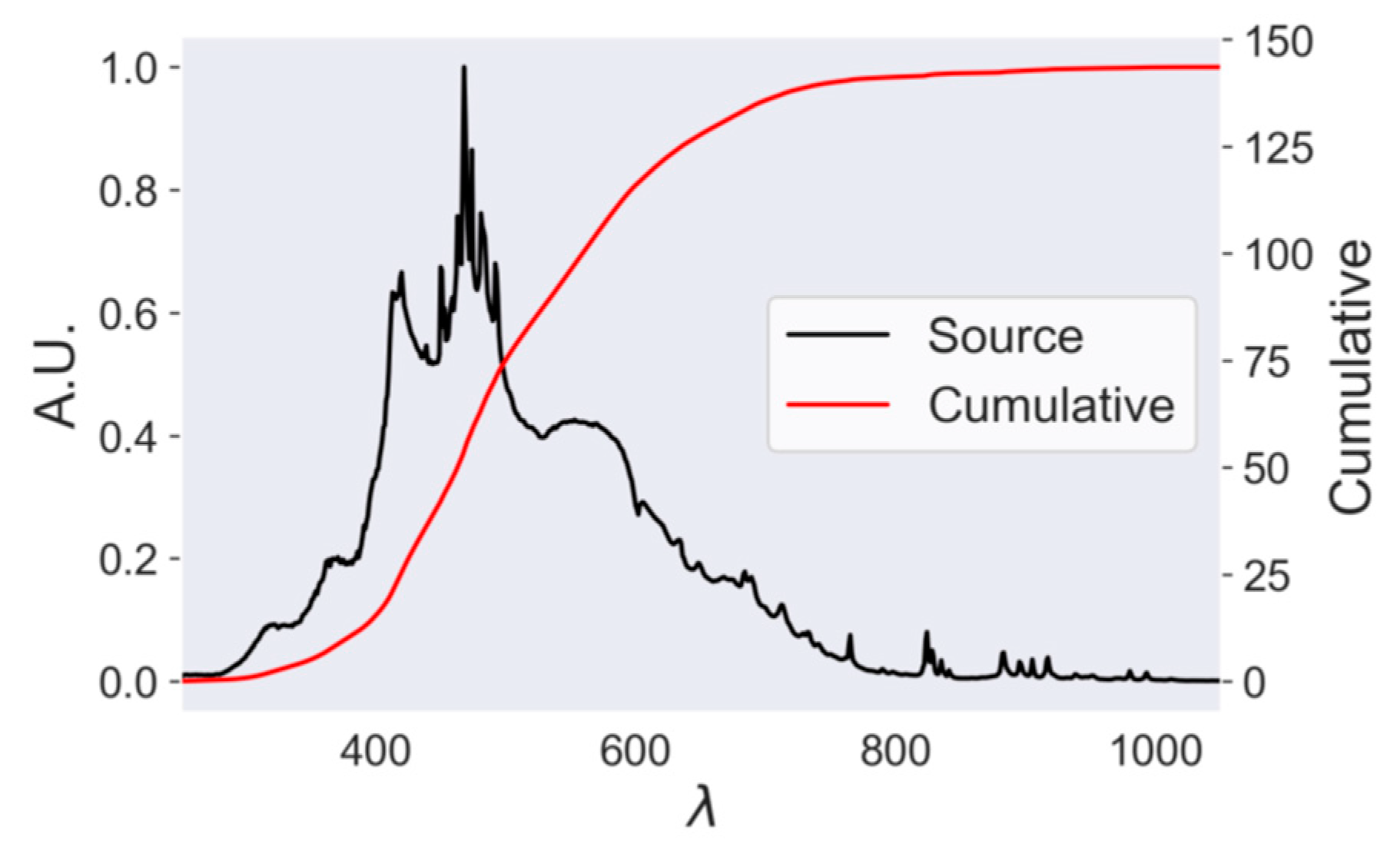
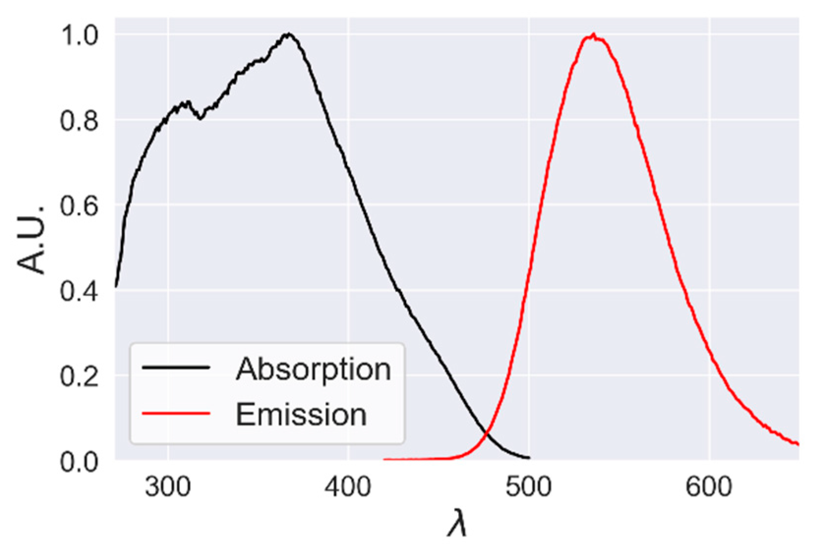
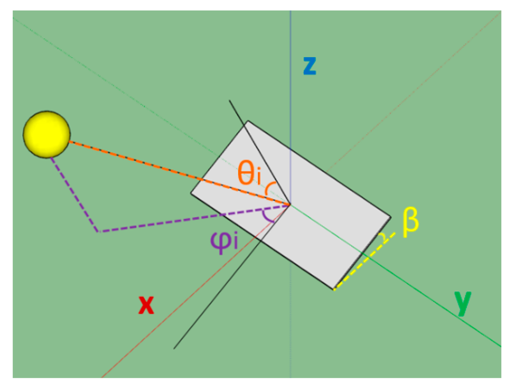
- Bundle: The initial position (xi, yi, zi) and direction (θi, ϕi) of the light vector are supplied, where xi is randomly determined between 0 and L, and yi is randomly determined between 0 and W. The starting volume number and particle object used for the simulation are also given. Lastly, λ is randomly sampled from the data shown in Figure 3.
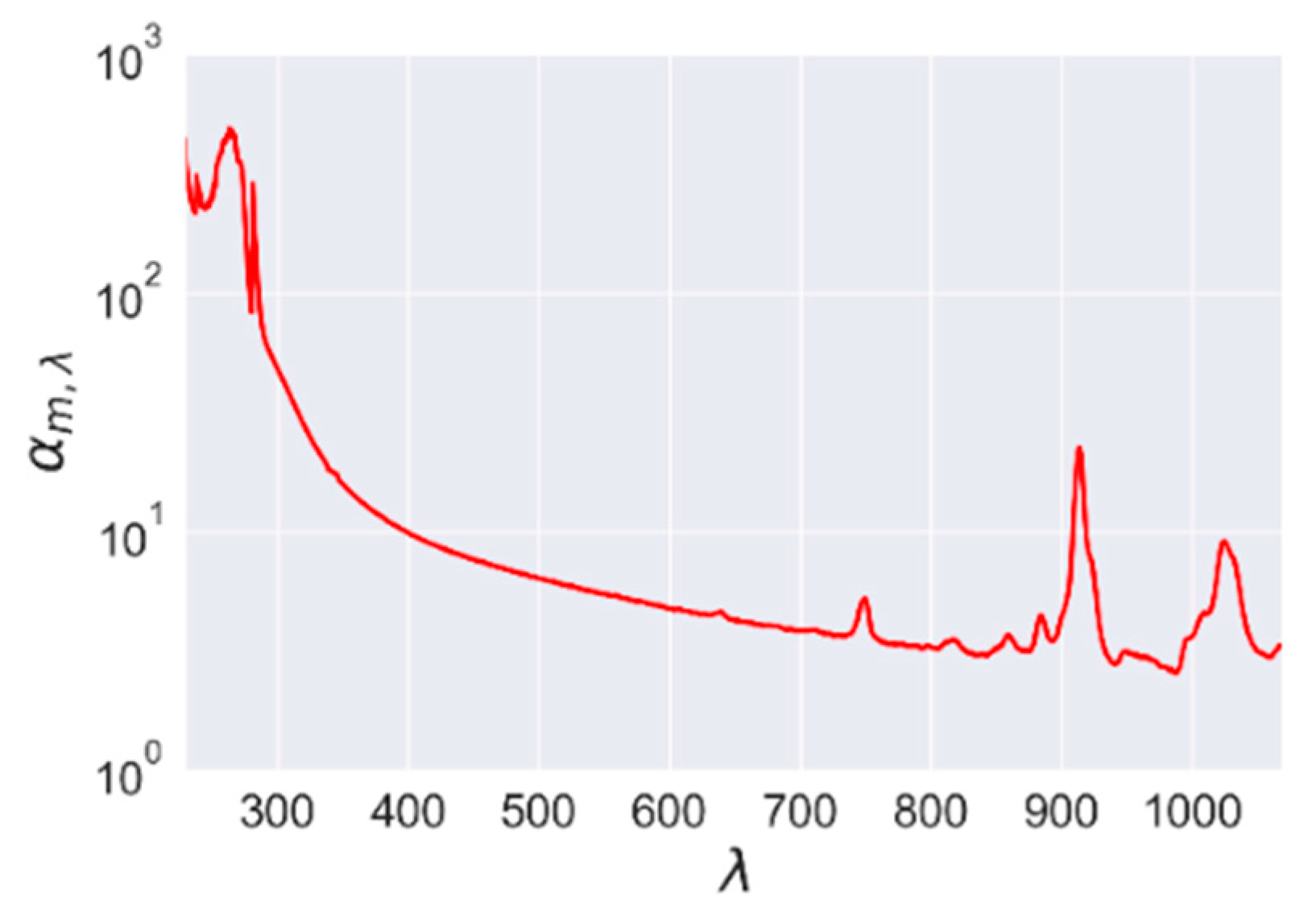
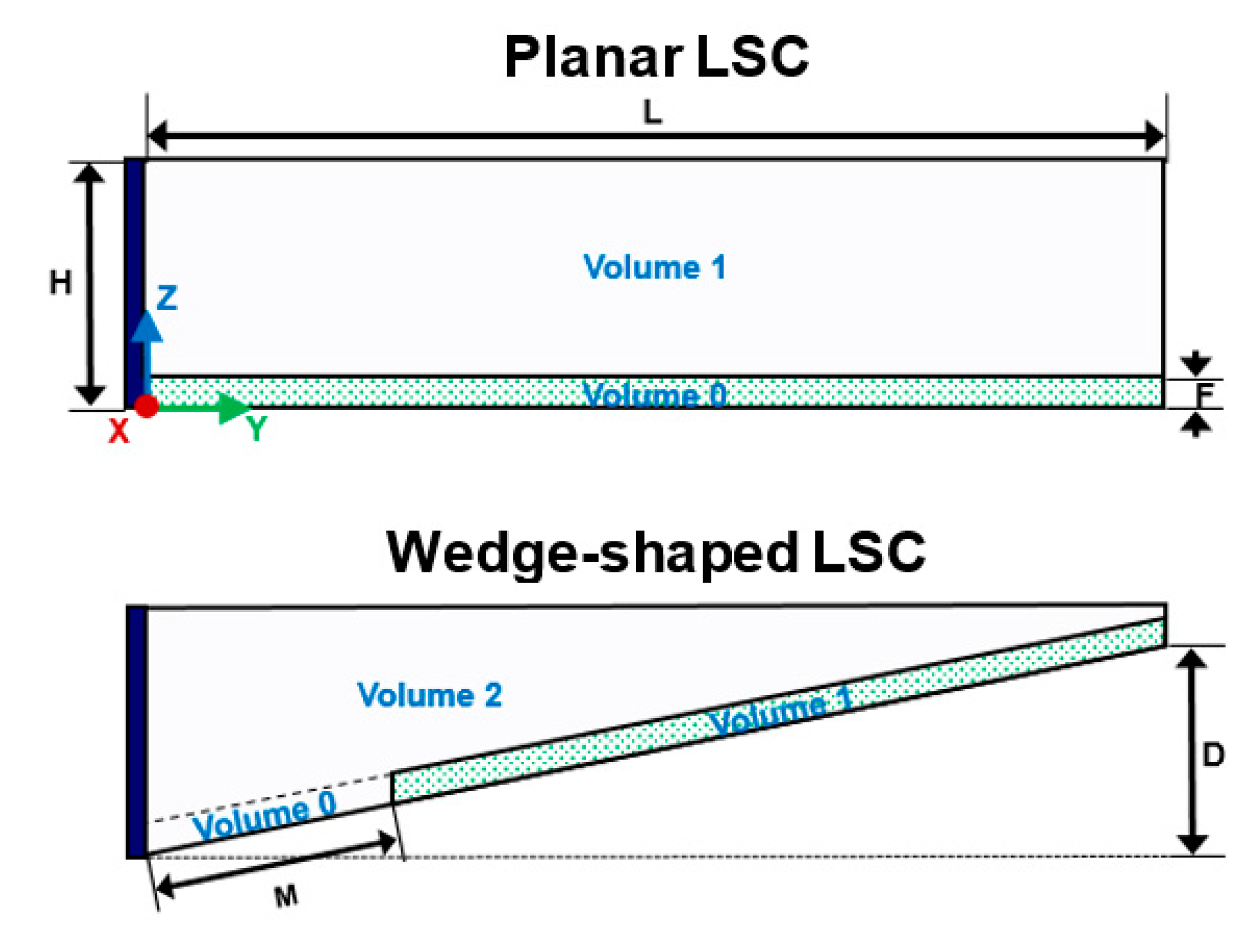
- Absorbing Volumes: The absorbing volumes in each case consist of transparent silicone (Dow Corning Sylgard 184) where and [40], with defined as seen in Figure 4. The Sellmeier equation (Equation (2)) is used to define index of refraction, and the boundaries that make up a particular volume are also supplied.
- Particle Volumes: All inputs to absorbing volumes are similar for particle volumes. In addition to these, particle volumes are also given an associated particle object.
- Opaque Boundaries: A set of points is input to form each boundary and the particular volume to which the boundaries belong is also indicated. All opaque boundaries are given a 5% likelihood of absorption (independent of λ), and reflection is handled specularly to represent the mirrors used (3M enhanced specular reflector).
- Transparent Boundaries: Only the points making up a transparent boundary and the parent volume object are input.
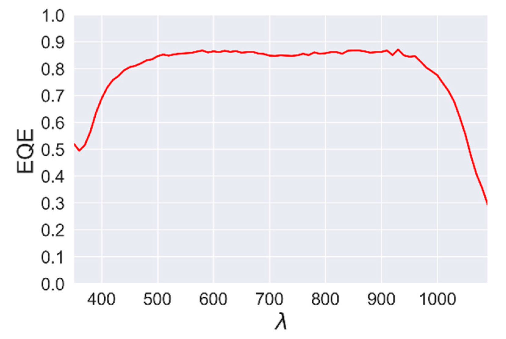
- PV Boundaries: PV boundaries are given a similar set of characteristics to opaque boundaries, but the EQE of the solar cells used in this paper is also provided as seen in Figure 9. If an IQE was known, this would have also been specified and reflection would be handled diffusely. With IQE unknown, reflected bundles are assumed to be lost at the solar cell to be conservative and EQE is used in place of IQE.
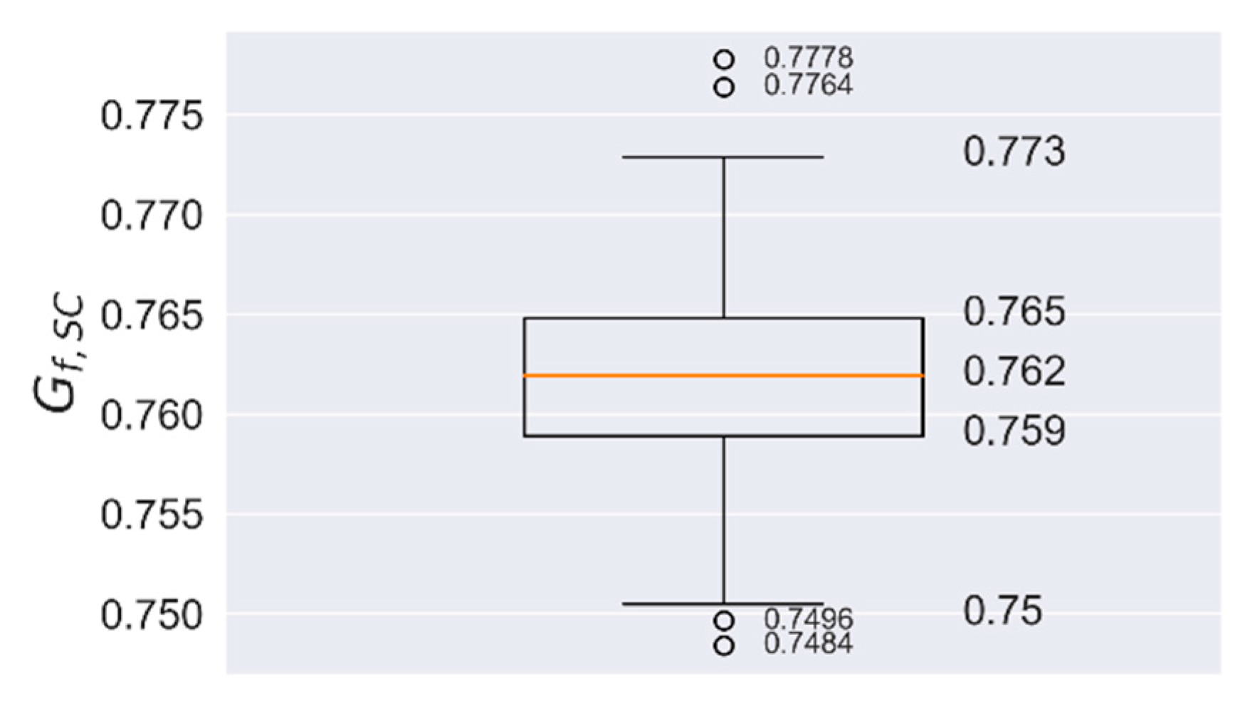
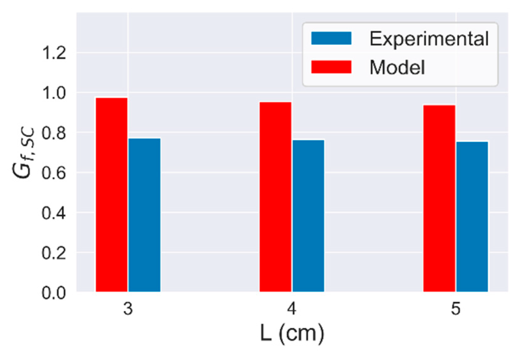
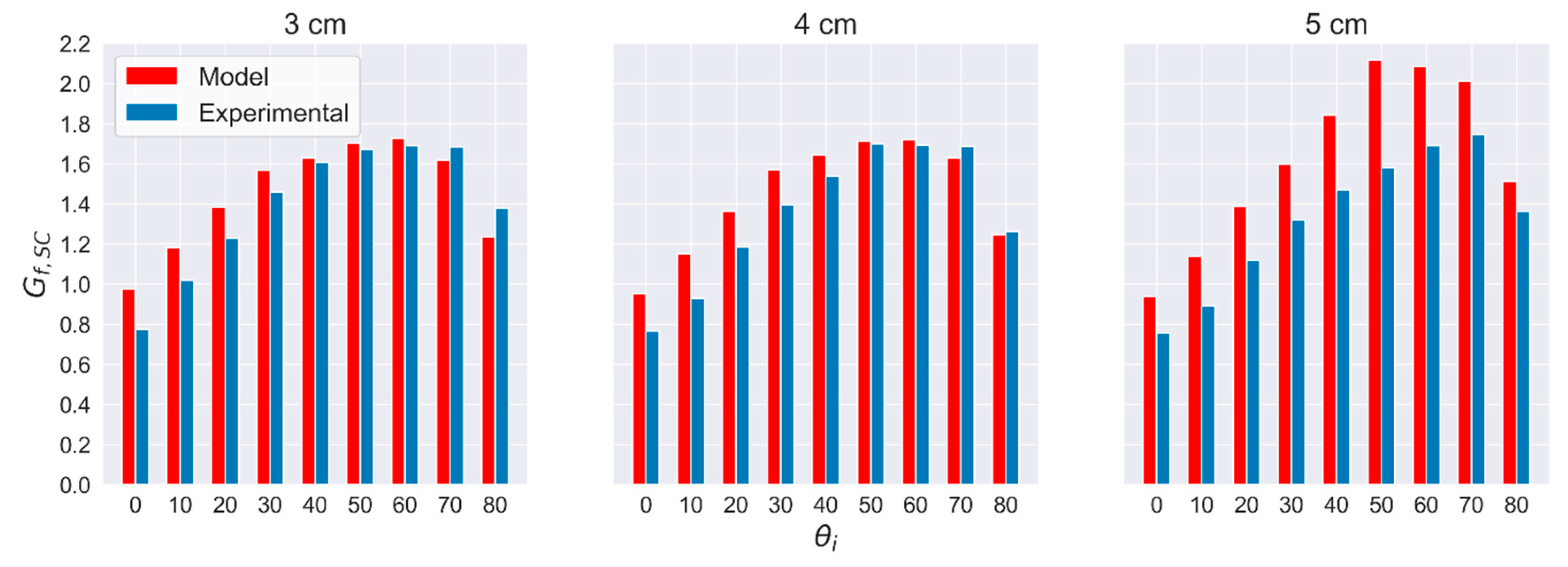
5.2. Discussion of Validation Study Results
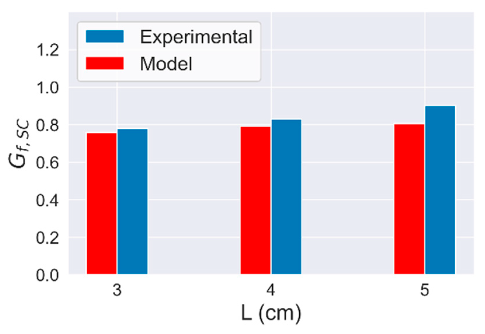
- , as a function of length, L;
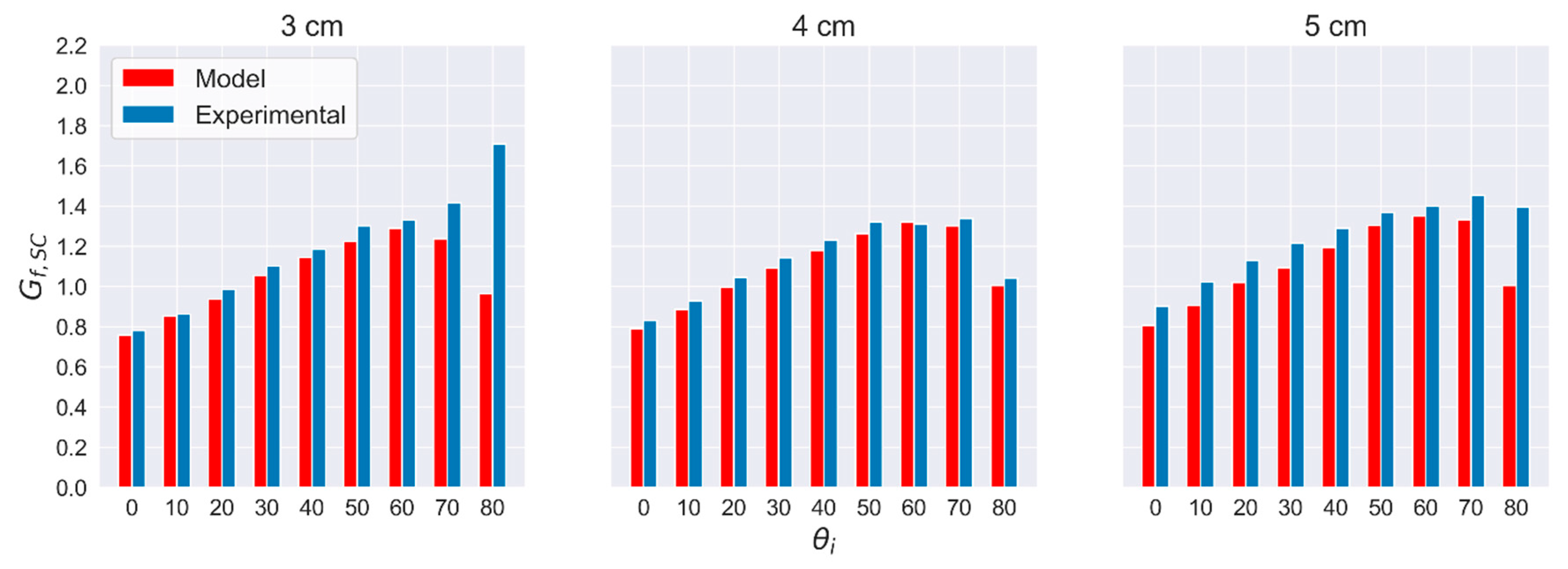
- as a function of polar incidence angle, θi and L;
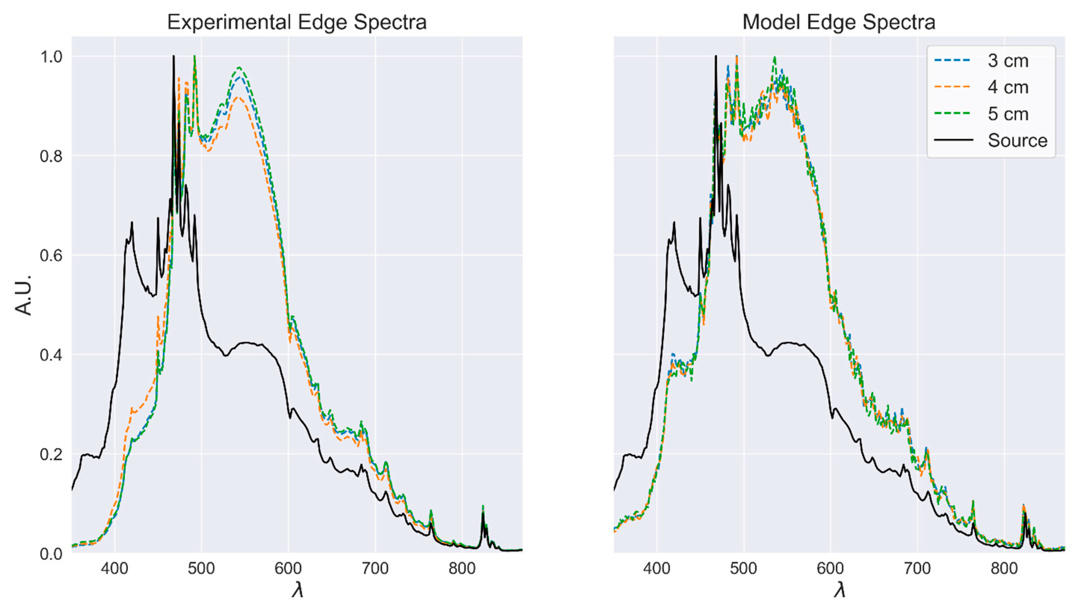
- PV edge spectra as a function of L.
- as a function of L;
- as a function of θi and L;
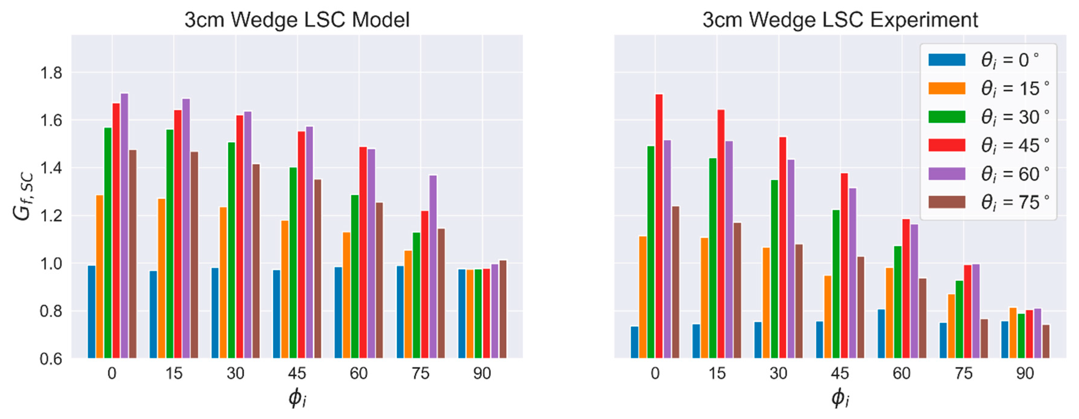
- as a function of polar and azimuthal incidence angle, θi and ϕi.
5.2.1. Discussion of Validation Study Results for Planar LSCs
5.2.2. Discussion of Validation Study Results for Wedge-Shaped LSCs
6. Conclusions
Supplementary Materials
Author Contributions
Funding
Data Availability Statement
Conflicts of Interest
References
- Hoegh-Guldberg, O.; Jacob, D.; Taylor, M.; Bindi, M.; Brown, S.; Camilloni, I.; Diedhiou, A.; Djalante, R.; Ebi, K.L.; Engelbrecht, F.; et al. Chapter 3: Impacts of 1.5 °C global warming on natural and human systems. In Global Warming of 1.5 °C. An IPCC Special Report on the Impacts of Global Warming of 1.5 °C above Pre-industrial Levels and Related Global Greenhouse Gas Emission Pathways; Intergovernmental Panel on Climate Change: Geneva, Switzerland, 2018; pp. 175–311. [Google Scholar]
- U.S. Energy Information Administration. International Energy Outlook 2019. Available online: https://www.eia.gov/outlooks/ieo/pdf/ieo2019.pdf (accessed on 13 January 2021).
- Global Building Envelope Market Size, Status and Forecast 2019–2025. Market. Research Consultant and Research Reports QY Research. Available online: www.qyresearch.com/index/detail/1357654/global-building-envelope-market (accessed on 13 January 2021).
- IEA; UNEP. International Energy Agency and the United Nations Environment Program—Global Status Report 2018: Towards A Zero-emission, Efficient and Resilient Buildings and Construction Sector; IEA: Paris, France; UNEP: Nairobi, Kenya, 2018; p. 325. [Google Scholar]
- California Public Utilities Commission. CA Energy Efficiency Strategic Plan. 2018. Available online: http://www.cpuc.ca.gov/General.aspx?id=4125 (accessed on 13 January 2021).
- Metzger, J. Historic Climate Leadership and Community Protection Act Signed into NYS Law. N. Y. State Senate. Available online: www.nysenate.gov/newsroom/press-releases/jen-metzger/historic-climate-leadership-and-community-protection-act-signed (accessed on 18 July 2019).
- European Commission. Nearly Zero-Energy Buildings. 2018. Available online: https://ec.europa.eu/energy/en/topics/energy-efficiency/buildings/nearly-zero-energy-buildings (accessed on 13 January 2021).
- Gammal, A.E.; Mueller, D.; Buerkstuemmer, H.; Vignal, R.; Macé, P. Technical evaluation of BIPV power generation potential in EU-28. In Proceedings of the 32nd European Photovoltaic Solar Energy Conference and Exhibition, Munich, Germany, 13 January 2016; pp. 2518–2522. [Google Scholar]
- Global Industry Analysts. Global Building Integrated Photovoltaics (BiPV) Market to Reach $39.9 Billion by 2027. July 2020. Available online: https://www.reportlinker.com/p03037269/Global-Building-Integrated-Photovoltaics-BIPV-Industry.html?utm_source=GNW (accessed on 13 January 2021).
- Skea, J.; Van Diemen, R.; Hannon, M.; Gazis, E.; Rhodes, A. Building Integrated Photovoltaics. In Energy Innovation for the Twenty-First Century: Accelerating the Energy Revolution; Skea, J., Ed.; Chapter 10; Edward Elgar Publishing: Cheltenham, UK, 2019. [Google Scholar]
- Bonomo, P.; Zanetti, I.; Frontini, F. BIPV products overview for solar building skin. In Proceedings of the 33rd European Photovoltaic Solar Energy Conference and Exhibition, Amsterdam, The Netherlands, 29 September 2017. [Google Scholar]
- Zanetti, B.; Bonomo, P.; Frontini, F.; Saretta, E.; van den Donker, M.; Vossen, F.; Folkerts, W. Building Integrated Photovoltaics: Product Overview for Solar Building Skins. 2017. Available online: https://resources.solarbusinesshub.com/images/reports/179.pdf (accessed on 13 January 2021).
- Goetzberger, A.; Greubel, W. Solar energy conversion with fluorescent collectors. Appl. Phys. 1977, 139, 123–139. [Google Scholar] [CrossRef]
- Weber, W.H.; Lambe, J. Luminescent greenhouse collector for solar radiation. Appl. Opt. 1976, 15, 2299–2300. [Google Scholar] [CrossRef] [PubMed]
- Carrascosa, M.; Unamuno, S.; Agullo-Lopez, F. Monte carlo simulation of the performance of PMMA luminescent solar collectors. Appl. Opt. 1983, 22, 3236. [Google Scholar] [CrossRef] [PubMed]
- Hughes, M.D.; Maher, C.; Borca-Tasciuc, D.-A.; Polanco, D.; Kaminski, D. Performance comparison of wedge-shaped and planar luminescent solar concentrators. Renew. Energy 2013, 52, 266–272. [Google Scholar] [CrossRef]
- Hughes, M.D.; Smith, D.E.; Borca-Tasciuc, D.-A. Performance of wedge-shaped luminescent solar concentrators employing phosphor films and annual energy estimation case studies. Renew. Energy 2020, 160, 513–525. [Google Scholar] [CrossRef]
- Inman, R.H.; Shcherbatyuk, G.V.; Medvedko, D.; Gopinathan, A.; Ghosh, S. Cylindrical luminescent solar concentrators with near-infrared quantum dots. Opt. Express 2011, 19, 24308. [Google Scholar] [CrossRef]
- Rafiee, M.; Chandra, S.; Ahmed, H.; Mccormack, S.J. An overview of various configurations of luminescent solar concentrators for photovoltaic applications. Opt. Mater. 2019, 91, 212–227. [Google Scholar] [CrossRef]
- Mazzaro, R.; Vomiero, A. The renaissance of luminescent solar concentrators: The role of inorganic nanomaterials. Adv. Energy Mater. 2018, 8, 1801903. [Google Scholar] [CrossRef]
- Delgado-Sanchez, J.M. Luminescent solar concentrators: Photo-stability analysis and long-term perspectives. Sol. Energy Mater. Sol. Cells 2019, 202, 110134. [Google Scholar] [CrossRef]
- Hughes, M.D.; Borca-Tasciuc, D.A.; Kaminski, D.A. Highly efficient luminescent solar concentrators employing commercially available luminescent phosphors. Sol. Energy Mater. Sol. Cells 2017, 171, 293–301. [Google Scholar] [CrossRef]
- De Boer, D.K.G.; Broer, D.J.; Debije, M.G.; Keur, W.; Meijerink, A.; Ronda, C.R.; Verbunt, P.P.C. Progress in phosphors and filters for luminescent solar concentrators. Opt. Express 2012, 20, A395–A405. [Google Scholar] [CrossRef] [PubMed]
- Duncan, E.S. lsclib: Library for Evaluating the Performance of Luminescent Solar Concentrators. Available online: https://github.com/duncanesmith/lsclib (accessed on 13 January 2021).
- Leow, S.W.; Corrado, C.; Osborn, M.; Carter, S.A. Monte carlo ray-tracing simulations of luminescent solar concentrators for building integrated photovoltaics. In Proceedings of the High and Low Concentrator Systems for Solar Electric Applications, San Diego, CA, USA, 9 September 2013; Volume 8821, p. 882103. [Google Scholar]
- Şahin, D.; Ilan, B.; Kelley, D.F. Monte-carlo simulations of light propagation in luminescent solar concentrators based on semiconductor nanoparticles. J. Appl. Phys. 2011, 110, 33108. [Google Scholar] [CrossRef]
- Bomm, J.; Büchtemanna, A.; Chatten, A.J.; Boseb, R.; Farrell, D.J.; Chan, N.L.A.; Xiao, Y.; Slooff, L.H.; Meyer, T.; Meyer, A.; et al. Fabrication and full characterization of state-of-the-art quantum dot luminescent solar concentrators. Sol. Energy Mater. Sol. Cells 2011, 95, 2087–2094. [Google Scholar] [CrossRef]
- Zhang, B.; Yang, H.; Warner, T.; Mulvaney, P.; Rosengarten, G.; Wong, W.W.H.; Ghiggino, K.P. A luminescent solar concentrator ray tracing simulator with a graphical user interface: Features and applications. Methods Appl. Fluoresc. 2020. [Google Scholar] [CrossRef] [PubMed]
- Kerrouche, A.; Hardy, D.A.; Ross, D.W.; Richards, B.S. Luminescent solar concentrators: From experimental validation of 3D ray-tracing simulations to coloured stained-glass windows for BIPV. Sol. Energy Mater. Sol. Cells 2014, 122, 99–106. [Google Scholar] [CrossRef]
- Farrell, D.J. Pvtrace: Optical Ray Tracing for Luminescent Materials and Spectral Converter Photovoltaic Devices. Available online: https://github.com/danieljfarrell/pvtrace (accessed on 13 January 2021).
- Jakubowski, K.; Huang, C.-S.; Gooneie, A.; Boesel, L.F.; Heuberger, M.; Hufenus, R. Luminescent solar concentrators based on melt-spun polymer optical fibers. Mater. Des. 2020, 189, 108518. [Google Scholar] [CrossRef]
- Moraitis, P.; De Boer, D.K.G.; Prins, P.T.; Donega, C.D.M.; Neyts, K.; Van Sark, W.G. Should anisotropic emission or reabsorption of nanoparticle luminophores be optimized for increasing luminescent solar concentrator efficiency? Sol. RRL 2020, 4, 1–7. [Google Scholar] [CrossRef]
- Videira, J.J.; Bilotti, E.; Chatten, A.J. Cylindrical array luminescent solar concentrators: Performance boosts by geometric effects. Opt. Express 2016, 24, 1188. [Google Scholar] [CrossRef]
- Farrell, D.J. Pvtrace: Optical Ray Tracing for Luminescent Materials and Spectral Converter Photovoltaic Devices. 006 Coatings. Available online: https://github.com/danieljfarrell/pvtrace/blob/master/examples/006%20Coatings.ipynb (accessed on 13 January 2021).
- Farrell, D.J. Pvtrace: Optical Ray Tracing for Luminescent Materials and Spectral Converter Photovoltaic Devices. 005 Geometry. Available online: https://github.com/danieljfarrell/pvtrace/blob/master/examples/005%20Geometry.ipynb (accessed on 13 January 2021).
- Farrell, D.J. Pvtrace: Optical Ray Tracing for Luminescent Materials and Spectral Converter Photovoltaic Devices. 002 Materials. Available online: https://github.com/danieljfarrell/pvtrace/blob/master/examples/002%20Materials.ipynb (accessed on 13 January 2021).
- Hughes, M.D.; Wang, S.-Y.; Borca-Tasciuc, D.-A.; Kaminski, D.A. Analysis of ultra-thin crystalline silicon solar cells coupled to a luminescent solar concentrator. Sol. Energy 2015, 122, 667–677. [Google Scholar] [CrossRef]
- Newport Corporation. 1600 W Oriel Solar Simulator 92193 Datasheet. Available online: https://www.artisantg.com/info/Oriel_SolarSimulator_Datasheet.pdf (accessed on 13 January 2021).
- Mahan, J.R. The Monte Carlo Ray-Trace Method in Radiation Heat Transfer and Applied Optics; John Wiley & Sons Ltd.: Hoboken, NJ, USA, 2019. [Google Scholar]
- Schneider, F.; Draheim, J.; Kamberger, R.; Wallrabe, U. Process and material properties of polydimethylsiloxane (PDMS) for Optical MEMS. Sens. Actuators A Phys. 2009, 151, 95–99. [Google Scholar] [CrossRef]
- Dow Corning. Sylgard 184 Silicone Elastomer Technical Datasheet. Available online: https://www.dow.com/content/dam/dcc/documents/en-us/productdatasheet/11/11-31/11-3184-sylgard-184-elastomer.pdf?iframe=true (accessed on 13 January 2021).
- Hughes, M.D.; Borca-Tasciuc, D.-A.; Kaminski, D.A. Method for modeling radiative transport in luminescent particulate media. Appl. Opt. 2016, 55, 3251–3260. [Google Scholar] [CrossRef] [PubMed]
- McIntosh, K.R.; Cotsell, J.N.; Cumpston, J.S.; Norris, A.W.; Powell, N.E.; Ketola, B.M. An optical comparison of silicone and EVA encapsulants for conventional silicon PV modules: A ray-tracing study. In Proceedings of the 2009 34th IEEE Photovoltaic Specialists Conference (PVSC), Philadelphia, PA, USA, 12 June 2009; Volume 34, no. 2. pp. 1649–1654. [Google Scholar]
- Van Verth, J.M.; Bishop, L.M. Orientation representation. In Essential Mathematics for Games & Interactive Applications, 2nd ed.; Morgan Kaufmann Publishers: Burlington, MA, USA, 2008; pp. 173–202. [Google Scholar]
- Gillies, S. Shapely: Manipulation and Analysis of Geometric Objects. 2007. Available online: https://pypi.org/project/Shapely/ (accessed on 13 January 2021).
- McEvoy, A.; Castaner, L.; Markvart, T. Principles of solar cell operation. In Solar Cells—Materials, Manufacture and Operation, 2nd ed.; Chapter IA-1; Elsevier: Amsterdam, The Netherlands, 2013; pp. 3–24. [Google Scholar]
- PhosphorTech Corporation. High Performance LED Phorsphors for High Power LEDs. Available online: https://phosphor-tech.com/products/led-phosphors/ (accessed on 13 January 2021).
- Digi-Key Electronics. IXOLARTM High Efficiency SolarBIT Datasheet KXOB22-04X3. Available online: https://ixapps.ixys.com/DataSheet/KXOB22-04X3-DATA-SHEET-20110808.pdf (accessed on 13 January 2021).


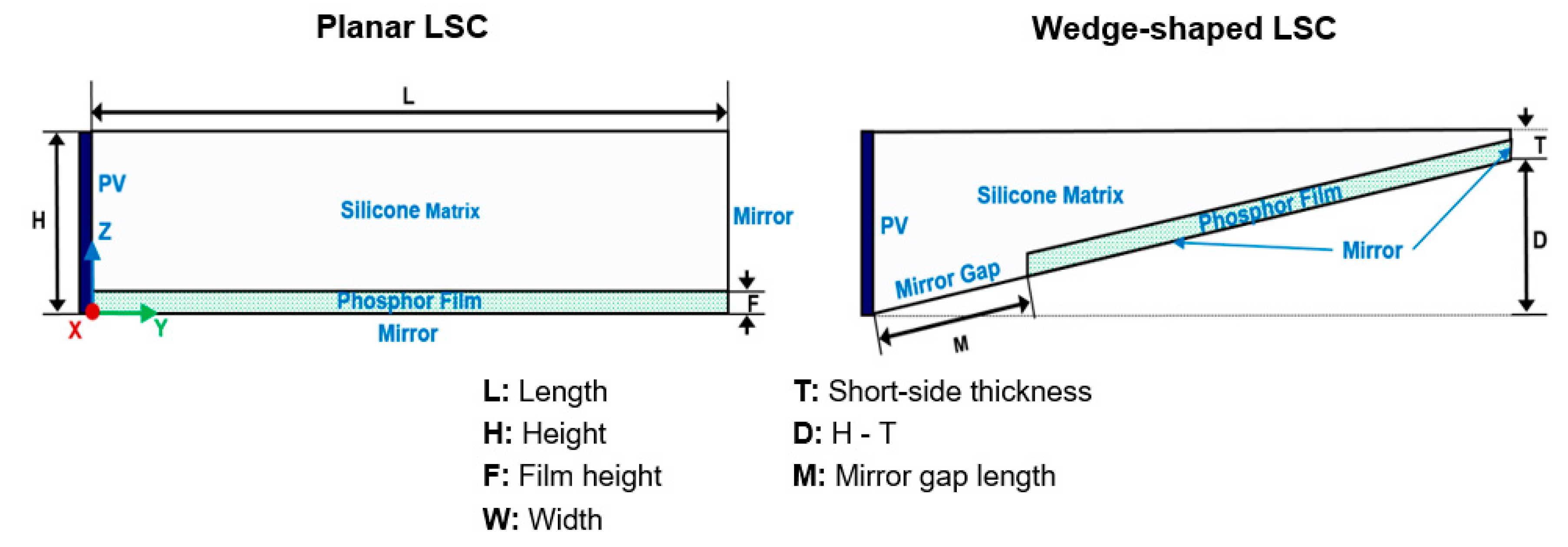
| LSC Geometry | L | H | F | W | M | T | D |
|---|---|---|---|---|---|---|---|
| Planar | 31.0 * | 7 | 1 | 22 | 0 | 7 | 0 |
| 42.0 * | 7 | 1 | 22 | 0 | 7 | 0 | |
| 50 | 4.5 † | 1 | 22 | 0 | 7 | 0 | |
| Wedge | 31.1 * | 7 | 1 | 22.6 | 5.77 | 1.03 | 5.97 |
| 37.2 * | 7 | 1 | 22.3 | 5.37 | 1.09 | 5.91 | |
| 50.3 | 7 | 0.98 | 24.3 | 7.71 | 0.99 | 6.01 |
Publisher’s Note: MDPI stays neutral with regard to jurisdictional claims in published maps and institutional affiliations. |
© 2021 by the authors. Licensee MDPI, Basel, Switzerland. This article is an open access article distributed under the terms and conditions of the Creative Commons Attribution (CC BY) license (http://creativecommons.org/licenses/by/4.0/).
Share and Cite
Smith, D.E.; Hughes, M.D.; Patel, B.; Borca-Tasciuc, D.-A. An Open-Source Monte Carlo Ray-Tracing Simulation Tool for Luminescent Solar Concentrators with Validation Studies Employing Scattering Phosphor Films. Energies 2021, 14, 455. https://doi.org/10.3390/en14020455
Smith DE, Hughes MD, Patel B, Borca-Tasciuc D-A. An Open-Source Monte Carlo Ray-Tracing Simulation Tool for Luminescent Solar Concentrators with Validation Studies Employing Scattering Phosphor Films. Energies. 2021; 14(2):455. https://doi.org/10.3390/en14020455
Chicago/Turabian StyleSmith, Duncan E., Michael D. Hughes, Bhakti Patel, and Diana-Andra Borca-Tasciuc. 2021. "An Open-Source Monte Carlo Ray-Tracing Simulation Tool for Luminescent Solar Concentrators with Validation Studies Employing Scattering Phosphor Films" Energies 14, no. 2: 455. https://doi.org/10.3390/en14020455
APA StyleSmith, D. E., Hughes, M. D., Patel, B., & Borca-Tasciuc, D.-A. (2021). An Open-Source Monte Carlo Ray-Tracing Simulation Tool for Luminescent Solar Concentrators with Validation Studies Employing Scattering Phosphor Films. Energies, 14(2), 455. https://doi.org/10.3390/en14020455