Deep RNN-Based Photovoltaic Power Short-Term Forecast Using Power IoT Sensors ^†

Abstract

Photovoltaic (PV) power fluctuations caused by weather changes can lead to short-term mismatches in power demand and supply. Therefore, to operate the power grid efficiently and reliably, short-term PV power forecasts are required against these fluctuations. In this paper, we propose a deep RNN-based PV power short-term forecast. To reflect the impact of weather changes, the proposed model utilizes the on-site weather IoT dataset and power data, collected in real-time. We investigated various parameters of the proposed deep RNN-based forecast model and the combination of weather parameters to find an accurate prediction model. Experimental results showed that accuracies of 5 and 15 min ahead PV power generation forecast, using 3 RNN layers with 12 time-step, were 98.0% and 96.6% based on the normalized RMSE, respectively. Their R²-scores were 0.988 and 0.949. In experiments for 1 and 3 h ahead of PV power generation forecasts, their accuracies were 94.8% and 92.9%, respectively. Also, their R²-scores were 0.963 and 0.927. These experimental results showed that the proposed deep RNN-based short-term forecast algorithm achieved higher prediction accuracy.

1. Introduction

Most of the electrical energy was supplied through fossil fuels. As the use of fossil fuels for power generation increases, concern for environmental pollution increases. Accordingly, unexhausted and clean renewable energy, such as solar energy and wind energy, becomes more significant and attracts more attention. The International Renewable Energy Agency (IRENA) reported that the world renewable energy capacity increased to 2537 GW in 2019 [1]. Solar energy is one of the promising renewable resources as a substitute for fossil fuels. In particular, the photovoltaic (PV) system steeply increased more than 14 times over 10 years, the capacity of which was from 41.5 GW in 2010 to 586.4 GW in 2019.

As the portion of PV power in the total electrical energy increases, the impact of PV power generation on the power grid is also increasing. PV power fluctuates rapidly with daytime weather changes due to cloud shadows and rainfalls [2]. This PV power fluctuation penetrates the power grid, causing a short-term mismatch between power supply and demand. It leads to instability and inefficiency of the power grid operation. Managing a power grid stably and efficiently requires short-term PV power forecasts to respond to PV power fluctuation [3,4,5].

The statistical and machine learning methods, such as ARMA (Auto-Regressive Moving Average), ARIMA (Auto-Regressive Integrated Moving Average), and regression models, were studied to forecast PV power generation [6,7,8]. Various neural network approaches, like artificial neural networks (ANN), gray prediction model [9], BP-ANN model [10], and the radial basis function (RBF) network [11], were proposed. To further improve the accuracy of PV power prediction, hybrid models were developed [12,13]. Those previous studies were based on historical PV power and weather data and were not suitable for real-time short term PV forecasting.

The online sequential extreme learning machine with a forgetting mechanism (FOS-ELM) was introduced to the short-term PV power prediction [14]. Predicted data computed by a weather forecast model was used as input to the PV prediction model. However, it required a large amount of computation for weather forecasting. A hybrid one-day-ahead power forecasting model was proposed, combining wavelet transform, particle swarm optimization, and support vector machine (Hybrid WT-PSO-SVM) [15]. It used the actual power data from PV power system SCADA (Supervisory Control and Data Acquisition) and numerical weather forecast meteorological data for one year with one-hour time step. To forecast daily generated PV power, several LSTM-RNN models were studied [16]. Wavelet-based LSTM-DNN model was proposed [17], which used predicted temperature and solar radiation for the short-term PV power prediction. Also, to enhance the short-term (24 ahead) forecasting accuracy of distributed PV power output, an adaptive hybrid predictor subset selection strategy was proposed, which combined binary genetic algorithm (BGA) and support vector regression (SVR) [18]. For a real-time short-term PV power forecast, feature data were collected at 5-min intervals [19], where a weighted Gaussian process regression was proposed to detect outliers in the data for improving the prediction accuracy.

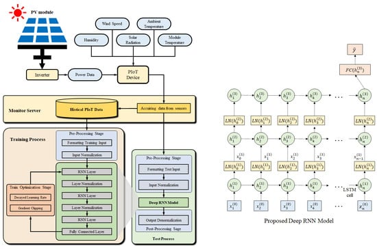
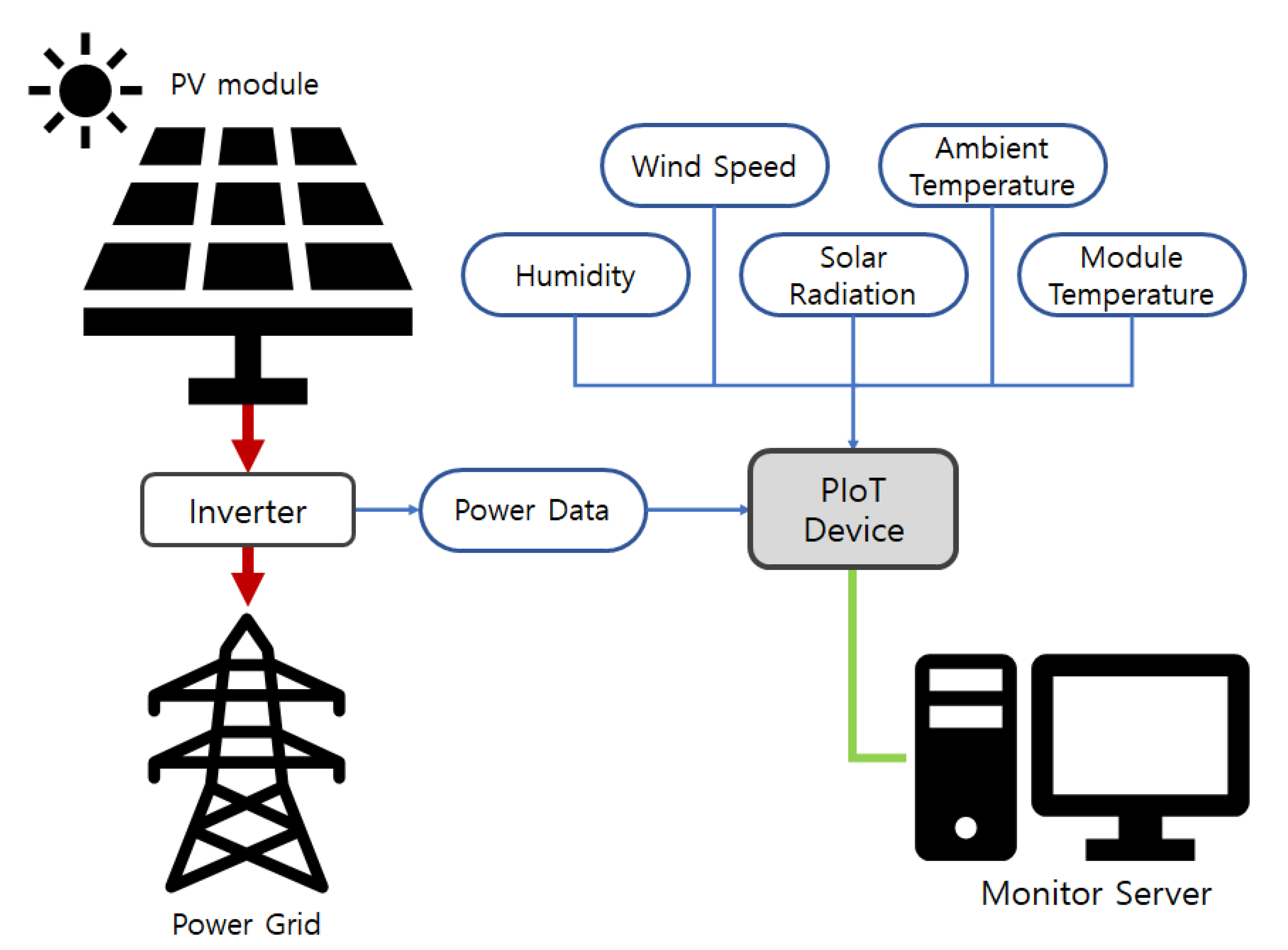
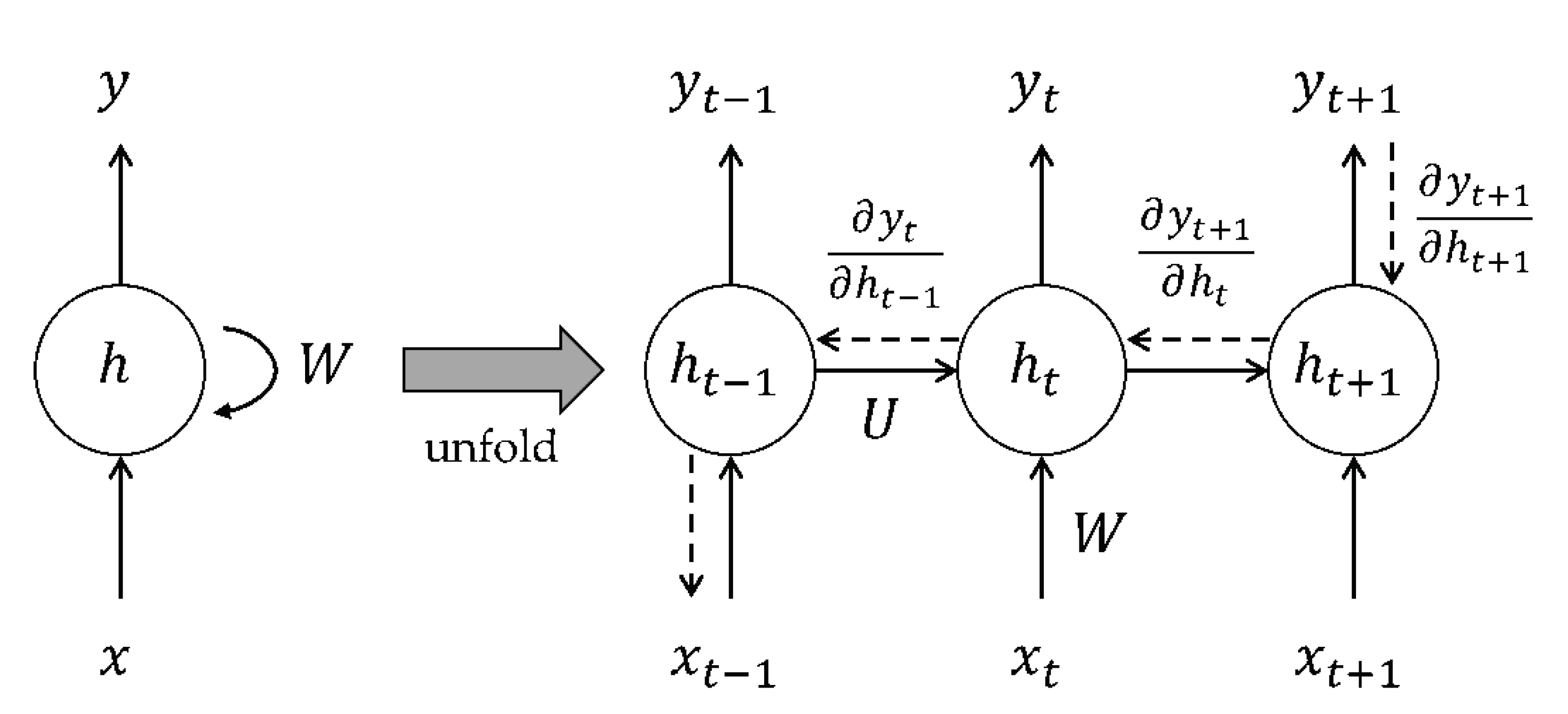
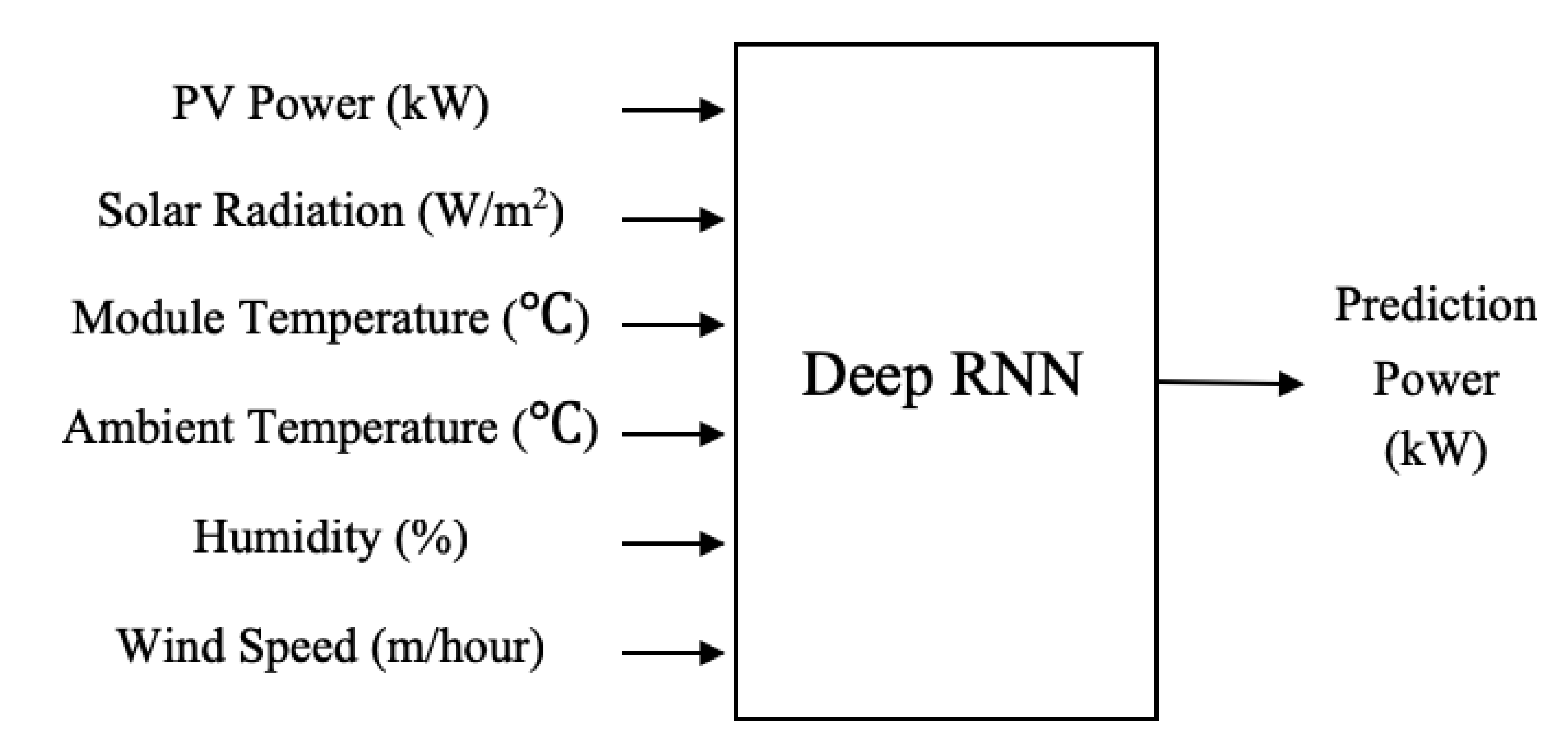
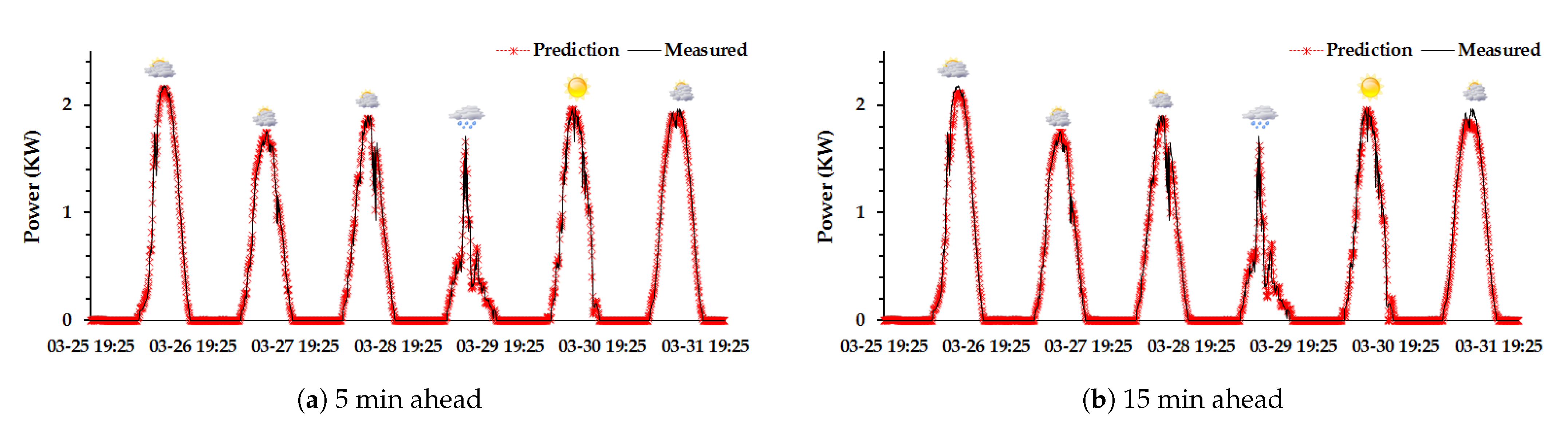
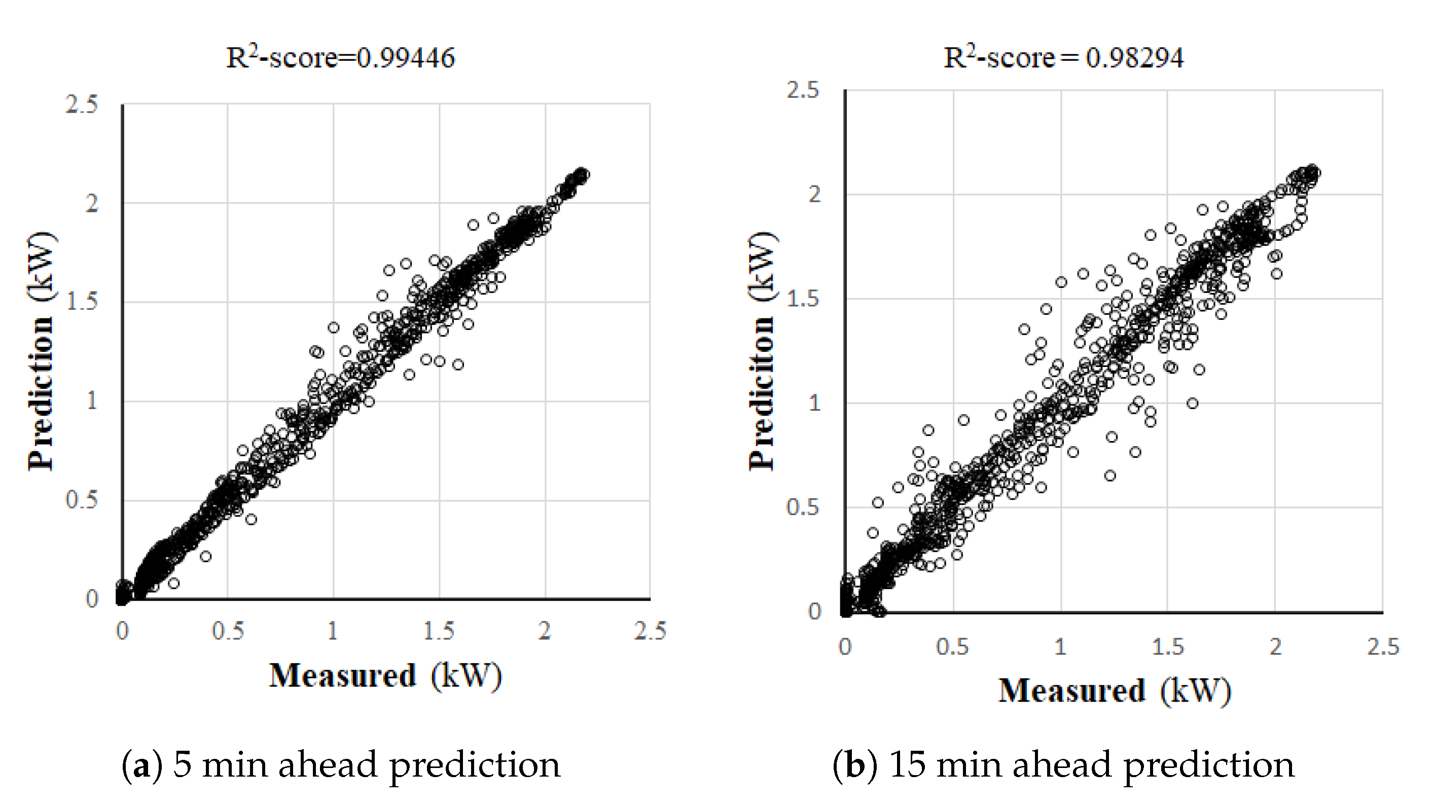
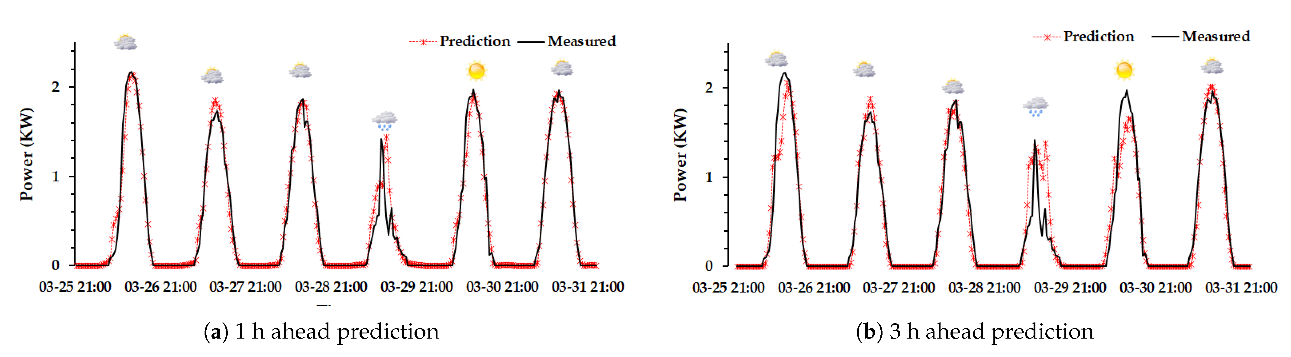
We propose a short-term PV power generation forecast algorithm based on the deep recurrent neural network (RNN) in the paper. To reflect the impact of weather changes, the proposed model utilizes the on-site weather IoT dataset and power data, collected in real-time. To build a model using low-cost and low-computation power, we used only IoT sensors without image data, such as solar radiation, module temperature, ambient temperature, wind speed, and humidity. In experiments, we investigated the best combination of parameters to improve forecast accuracy. The proposed deep-RNN consists of multiple RNN layers. Each RNN layer includes long-short term memory (LSTM) and layer normalization units. For experiments, a very short-term forecast algorithm predicts a power 5 or 15 min ahead. A short-term forecast algorithm also predicts a power 1 h or 3 h ahead. The experimental results showed that the very short-term forecast accuracy was 99.01% (nMAE)/98.02% (nRMSE) for 5 min ahead prediction and 98.16% (nMAE)/96.58% (nRMSE) for 15 min ahead prediction using three RNN layers. And the short-term prediction accuracy was 93.75% (nRMSE) and 96.6% (nMAE) for 1 h ahead prediction and 90.29% (nRMSE) and 94.7% (nMAE) for 3 h ahead prediction.

This paper organizes as follows. Section 2 describes the photovoltaic power generation system and Power IoT data. In Section 3, the short-term PV power forecasting algorithm based on deep-RNN is proposed. The experimental results and performance evaluation are discussed in Section 4, and then the conclusion is summarized in Section 5.

2. Collecting PV Power Datasets Using Power IoT Sensors

2.1. Photovoltaic Power Generation System with Power IoT Sensors

Since PV power systems use solar radiation to generate electricity, PV power is sensitive to weather changes. Therefore, on-site weather information as well as PV power data is needed to predict short-term PV power generation [20]. Various weather information providers like the Meteorological Administration (KMA) publish regularly observed weather data and weather forecasts. We may collect such data over the Internet. However, they are released at intervals of at least 1 h, so they are not suitable for short-term predictions. Since the published meteorological data are measured based on meteorological observations, it may differ from the on-site weather conditions of the solar system considered in this study.

To obtain PV power data and on-site weather information for this study, we adopt a data acquisition system using the PIoT (Power Internet of Things) device shown in Figure 1. PIoT devices measure the DC current and voltage to monitor generated PV power. Also, we use five IoT sensors to measure solar radiation, module temperature, ambient temperature, humidity, and wind speed. The collected PIoT data are transmitted and stored to the monitor server.

2.2. The Correlation Analysis of PIoT Data in the Photovoltaic System

In order to design a short-term forecast algorithm, it is important to select learning parameters. For PV power generation short-term forecast, we analyze the correlation between the generated power data and the PIoT data in a PV system and select the efficient parameters accordingly [21]. The Pearson correlation coefficient r is used for the correlation analysis as follows:

$$r=\frac{\sum (x-x^{\prime })(y-y^{\prime })}{\sqrt{\sum {(x-x^{\prime })}^2}\times \sqrt{\sum {(y-y^{\prime })}^2}}$$

(1)

where x and y are the individual samples and $x^{\prime }$ and $y^{\prime }$ are their sample means. Figure 2 shows the correlation between data parameters measured from PIoT sensors, including the power and weather data. In general, the PV power generation performance is related to solar irradiation, module temperature, and ambient temperature. However, wind speed and humidity are not taken into consideration since these are not directly related to the current and voltage equation of PV power generation. As shown in Figure 2, the humidity and wind speed have a relation to the module temperature, resulting in affecting the PV power generation indirectly [22,23]. They are less significant than solar radiation, module temperature, and ambient temperature. Depending on how far short-term prediction, the influence of the parameter will change. In this study, we investigate the prediction impacts of these parameters through experiments.

3. Short-Term PV Power Generation Forecast Based on Deep-RNN Using PIoT Data

3.1. The Review of RNN and LSTM

A general artificial neural network (ANN) consists of inputs and outputs that are independent of each other. In general, inputs and outputs of time-series applications are interdependent, so the ANN is known as unsuitable for them. A recurrent neural network (RNN) is proposed for the time-series applications, as shown in Figure 3 [24]. Unlike ANN, an RNN unit takes previous hidden states and present inputs as input and makes new current hidden states and outputs. During training, the RNN parameters are updated using the backpropagation through time (BPPT) algorithm [25], which is indicated by the dotted line in Figure 3.

Let’s consider an example of RNN as shown in Figure 3. The hidden state $h_t$ at time t can be calculated as follows, where the present input is $x_t$, the recurrent hidden state is $h_{t-1}$ at time $t-1$, $\sigma$ is the sigmoid function (or other non-linear functions like hyperbolic tangent and the rectified linear function), and W and U are the weight matrices and b is the biases:

$$\begin{array}{ccc}\hfill h_t& =& \hfill \sigma (W{x}_t+U{h}_{t-1}+b)\hfill \end{array}$$

(2)

$$\begin{array}{ccc}\hfill y_t& =& \hfill W{h}_t\hfill \end{array}$$

(3)

If the length of a data sequence in RNN increases, the training time of RNN drastically increases. Also, RNN output can converge into 0 or infinite, which is called a vanishing/exploding gradient problem. To overcome the vanishing/exploding gradient problem of the RNN model, the long-short term memory (LSTM) network is proposed [26]. The LSTM network consists of an LSTM cell, instead of an RNN cell, as shown in Figure 4. Different from RNN cells, the LSTM cell can determine whether to retain or discard the previous hidden states through a forget gate ($f_t$) and calculate current hidden states as output accordingly. The forget gate ($f_t$) is computed by the sigmoid function ($\sigma$) of the input data ($x_t$) and previous hidden state ($h_{t-1}$). According to the status of the previous cell ($C_{t-1}$), which is between 0 and 1, it is determined how much of the previous hidden state is accepted. If $C_{t-1}$ is zero, any value of the previous hidden state ($h_{t-1}$) is not accepted as an input. If it is one, all of the previous hidden state ($h_{t-1}$) is accepted. First, the forget gate $f_t$ at time t can be calculated as follows, where the forget gate weight is $W_f$ and the forget gate bias unit is $b_f$:

$$f_t=\sigma (W_f[h_{t-1},x_t]+b_f).$$

(4)

Second, the information value ($i_t$) and the new candidate value (${\tilde{C}}_t$) can be calculated as follows, where the information value and the new candidate weight are $W_i$ and $W_C$ and the information value and the new candidate bias are $b_f$ and $b_C$:

$$\begin{array}{ccc}\hfill i_t& =& \hfill \sigma (W_i[h_{t-1},x_t]+b_i)\hfill \end{array}$$

(5)

$$\begin{array}{ccc}\hfill {\tilde{C}}_t& =& \hfill tanh(W_C[h_{t-1},x_t]+b_C).\hfill \end{array}$$

(6)

Finally, the LSTM cell generates a new state value ($C_t$) that determines how much information is forgotten or kept at time $t+1$. The output decision $o_t$ at time t can be calculated as follows, where the output decision’s weight is $W_o$ and the output decision’s bias unit is $b_o$:

$$\begin{array}{ccc}\hfill C_t& =& \hfill f_t\times C_{t-1}+i_t\times {\tilde{C}}_t\hfill \end{array}$$

(7)

$$\begin{array}{ccc}\hfill o_t& =& \hfill \sigma (W_o[h_{t-1},x_t]+b_o).\hfill \end{array}$$

(8)

The current hidden state ($h_t$) is computed by the multiplying $o_t$ and the hyperbolic tangent of $C_t$.

$$h_t=o_t\times tanh(C_t)$$

(9)

3.2. Deep RNN-Based Short-Term Forecasting

For a short-term forecast of PV power generation, we propose a deep RNN with a multi-layer model as shown in Figure 5. After finishing the training process, the test process evaluates the performance of the deep RNN model using the test dataset. The proposed deep RNN model takes in input data measured by PIoT sensors, which are a PV power, solar radiation, module and ambient temperature, a humidity, and wind speed in the on-site, to forecast the short-term PV power generation as shown in Figure 6. Time-series sequence data is collected periodically through PIoT sensors. Before fed into the proposed model, it is applied to the pre-processing stage. At first, the collected sequence data is formatted to a requested interval to fit the input format of a short-term or very short-term forecast model. In the next, each formatted input data is normalized. In general, a photovoltaic system has the maximum generating electrical power capacity. Also, according to weather statistics, weather data generally vary within some range. The normalization of weather input data is computed as follows:

$$x_{norm}=\frac{x-x_{min}}{x_{max}-x_{min}}$$

(10)

where x is an input vector, $x_{norm}$ is the normalized input vector, $x_{max}$ is the maximum value of x, and $x_{min}$ is the minimum value of x. Input normalization helps to improve the accuracy and execution time of the training process [27].

The proposed deep RNN model consists of multi-layer RNN with layer normalization and one fully-connected layer. Figure 7 shows one example of a deep RNN, consisting of 3 layers with a layer normalization and one fully-connected layer. The input layer of RNN receives normalized input vectors computed in the pre-processing stage. In order to overcome the vanishing and the exploding problem of the RNN model, each RNN cell is configured with an LSTM cell introduced in Section 3.1. At the layer i, the output of the $t$th RNN cell is computed as follows, where $x_t^{i-1}$ is the output of the $t$th output of the $(i-1)$th RNN layer including the RNN cell and layer normalization computation:

$$h_t^{(i)}=\mathrm{LSTM}(x_t^{(i-1)},h_{t-1}^{(i)})\mathrm{where}t=1,2,\cdots ,n$$

(11)

In general, batch normalization is not suitable for the RNN model. Instead of batch normalization, layer normalization [28] is applied to the proposed model by computing the normalization statistics separately at each time step as follows, where $LN$ is the computation of layer normalization:

$$x_t^{(i)}=LN(h_{t1}^{(i)})\mathrm{where}t=1,2,\cdots ,n$$

(12)

The layer normalization at the tth time step, $LN(h_t)$, is computed as follows:

$$\begin{array}{ccc}\hfill LN(h_t)& =& \hfill f[\frac{g}{{\sigma }_t}\odot (h_t-{\mu }_t)+b]\hfill \end{array}$$

(13)

$$\begin{array}{ccc}\hfill {\mu }_t& =& \hfill \frac{1}{H}\sum _{j=1}^H{h}_{t,j}\hfill \end{array}$$

(14)

$$\begin{array}{ccc}\hfill {\sigma }_t& =& \hfill \frac{1}{H}\sum _{j=1}^H{(h_{t,j}-{\mu }_t)}^2\hfill \end{array}$$

(15)

where H is the number of hidden units in an LSTM cell. ⊙ is the element-wise multiplication between two vectors. b and g are bias and gain parameters of the same dimension as $h_t$. Layer normalization improves the training and test computation time in our model. Also, it can effectively stabilize the hidden state dynamics in RNN. Finally, a fully connected layer applied to the output of the last time-step LSTM makes PV power generation prediction. We optimize the proposed deep RNN model trained with backpropagation using an Adam optimizer [29] to minimize the prediction loss. Furthermore, we apply the decayed learning rate method in the training optimization stage. As the training epoch increases and the prediction loss decreases, the learning rate is decayed to approach the optimal point. Also, we apply the gradient clipping to our deep-RNN model in order to limit the magnitude of the gradient. It can make stochastic gradient descent (SGD) behave better in the vicinity of cliffs since cliffs commonly occur in recurrent neural networks. After optimizing the training, the inference model built based on deep-RNN is used to short-term predict PV power generation. Since validation and test datasets are normalized in the pre-processing stage, the predicted output should be denormalized to compare with the measured PV power.

4. Experimental Results

4.1. Experimental Environments and Performance Evaluation

For this study, we used a PV power platform, which consisted of 10 serial-connected solar panels on the roof of the Engineering Building in Konkuk University, Seoul, Korea, as shown in Figure 8. For the proposed deep RNN-based short-term PV power forecast model, we measured the on-site PV power and weather data using PIoT sensors installed in the PV power platform. The DC voltage and current of the PV system and the weather data such as solar radiation, module, and ambient temperature, humidity, and wind speed were collected using PIoT sensors summarized in

Table 1. Installed solar devices and PIoT sensors.

Parts	Device
Solar panels	10 serial-connected LG250S9W panels
Maximum electrical power	2.649 kW
Solar radiance sensor	SE1000-SEN-IRR-S1
Module temperature sensor	SE1000-SEN-TMOD-S2
Ambient temperature sensor	SE1000-SEN-TAMB-S2
Wind speed sensor	SE1000-SEN-WIND-S1
Humidity sensor	DY-HTT1

. We partitioned the whole data into 3 data sets: train, validation, and test set. The ratio of them is 3:1:1. We conducted the experiments on the Nvidia Tesla P100 server. The training parameters were presented in

Table 2. Training Model Parameters.

Parameters	Value
Learning Rate	0.01
Layers	3, 5, 7
Epochs	10,000
Time steps of RNN	12, 24, 36, 48

.

We trained the model in 10 times and tested these models, and then reported their average prediction accuracy. To evaluate the prediction accuracy, normalized Root Mean Square Error (nRMSE), normalized Mean Absolute Error (nMAE) for the maximum power capacity of a PV system, and R${}^2$-score were computed as follows [30]:

$$\mathrm{nRMSE}=\sqrt{\frac{1}{N}\sum _{i=1}^N\frac{{({\tilde{P}}_i-P_i)}^2}{P_m}}$$

(16)

$$\mathrm{nMAE}=\frac{1}{N}\sum _{i=1}^N\frac{|{\tilde{P}}_i-P_i|}{P_m}$$

(17)

$$R^2\text{-}\mathrm{score}=1-\frac{{\sum }_i{({\tilde{P}}_i-P_i)}^2}{{\sum }_i{(P_i-P^{{}^{\prime }})}^2}$$

(18)

where ${\tilde{P}}_i$ is the prediction power, $P_i$ is the measured power, $P_m$ is the maximum capacity of the PV power, and $P^{{}^{\prime }}$ is the mean of the measured power. nRMSE and nMAE can be represented as a percentage (%) since the normalized power, varying from 0 to 1, is used as inputs.

4.2. Experiment Results and Discussion

We designed a set of experiments composed of two groups: one for a very short-term forecast and the other for a short-term forecast model. Very short-term forecasting experiments were considered for 5-min and 15-min ahead predictions of PV power generation. For the short-term forecast, experiments were conducted concerning the 1 h ahead and the 3 h ahead forecast. To make the best short-term forecasting model, we performed experiments by varying the number of time steps of a RNN layer. In

Table 3. Results of the very short-term forecasting error by varying the number of RNN time steps.

Time Steps	nRMSE		nMAE
	5 min Ahead	15 min Ahead	5 min Ahead	15 min Ahead
12	0.0214371	0.0348593	0.0109102	0.0179979
24	0.0216388	0.0369868	0.0111218	0.0189269
36	0.0229877	0.0363113	0.0120307	0.0183018
48	0.0220876	0.0369531	0.0114320	0.0186102

, the results of the very short-term forecast were presented. The time interval of an RNN time step was 5 min. Typically the change of the weather features for 5 or 15 min was relatively less than that for a longer period like 1 h, 3 h, or one day. As shown in Table 3, the deep RNN-based forecast model using 12 time-steps achieved a smaller prediction error than ones with 24, 36, or 48 time-steps.

Table 4. Results of very short-term forecasting error by varying the number of RNN layers.

RNN Layers	nRMSE		nMAE
	5 min Ahead	15 min Ahead	5 min Ahead	15 min Ahead
3	0.0214371	0.0348592	0.0109102	0.0179979
5	0.0228140	0.0356600	0.0117408	0.0183442
7	0.0247898	0.0366400	0.0129337	0.0190659

showed the error of a very short-term forecast by varying the number of RNN layers. The deep RNN consisting of 3 layers achieved the best prediction accuracy. As the number of layers increases, the prediction accuracy was degraded a little. So, we chose the deep RNN consisting of 3 layers for overall experiments in the very short-term forecast. The 5 min ahead prediction accuracy of PV power generation was 98.9% (nMAE) and 97.9% (nRMSE). The 15 min ahead prediction accuracy of PV power was 98.2% (nMAE) and 96.5% (nRMSE) using 3-layer RNN with 12-time steps.

To forecast very short-term PV power generation, we used all of PIoT sensor data based on the correlation analysis in Section 2.2. Further experiments were conducted to find the best combination of PIoT sensors with minimal forecasting error.

Table 5. Very short-term forecasting errors according to PIoT sensors: P (Power), Solar (S), Wind Speed (WS), Humidity (H), Ambient Temperature (AT), Module Temperature (MT).

PIoT Sensor	nRMSE		nMAE
	5 min Ahead	15 min Ahead	5 min Ahead	15 min Ahead
P + S	0.0201445	0.0349844	0.0096700	0.0173440
P + WS	0.0205237	0.0342443	0.0099648	0.0168421
P + H	0.0211889	0.0375769	0.0106577	0.0197006
P + AT	0.0198681	0.0337223	0.0095489	0.0168570
P + MT	0.0195991	0.0339807	0.0093713	0.0168980
P + S + WS	0.0196118	0.0335514	0.0091331	0.0160464
P + S + H	0.0210492	0.0356164	0.0102950	0.0176773
P + S + AT	0.0197068	0.0350883	0.0094416	0.0174761
P + S + MT	0.0199925	0.0347033	0.0097225	0.0170862
ALL	0.0214371	0.0348592	0.0109102	0.0179979

showed a result of very short-term forecasting errors due to the combination of PIoT sensors. For the very short-term forecasting PV power, the combination of PV Power (P), Solar (S), and Wind Speed (WS) minimized the error compared to others. Short-term temperature changes can be further affected by wind speed. Using the selected PIoT sensor combination, the 5 min ahead prediction accuracy of PV power was improved to 99.1% (nMAE) and 98.0% (nRMSE). The 15 min ahead prediction accuracy of PV power was 98.4% (nMAE) and 96.6% (nRMSE) using 3-layer RNN with 12-time steps.

Figure 9 and Figure 10 showed the results of 5 and 15 min ahead forecast using the selected PIoT sensor combination for 3 different weather cases. The deep RNN-based forecast model used 3 RNN layers, 12 time-steps of RNN, and the sampling interval of 5 min. In Figure 11, the 5 and 15 min ahead forecast results of PV power generation during 6 consecutive days were presented, compared with the power measured in the PV platform. Even though the weather changed to a cloudy or rainy day, the prediction graph in Figure 11 showed the proposed model made reliable forecast results. The scatter graphs of the very short-term forecast were presented in Figure 12. R${}^2$-scores of 5 min and 15 min ahead forecast were 0.983 and 0.949, respectively.

For the short-term PV power generation forecast, the weather change during the longer period should be observed, since it will be related to the PV power generation trend during a half-day or a full day. In the experiments, it was predicted based on data collected during 6, 12, 18, or 24 h. For the short-term forecast, the sampling interval between two time-steps in RNN was a half hour (30 min) or one hour. If the samples every 5 min were used, the number of time-steps in RNN increased too large to degrade the overall prediction accuracy and to increase the training time.

Table 6. Results of short-term forecast errors of PV power generation.

(a) Sampling Interval: A Half Hour
RNN Layers	Time Steps	nRMSE		nMAE
		1 h Ahead	3 h Ahead	1 h Ahead	3 h Ahead
3	12	0.057695	0.092774	0.032357	0.059011
	24	0.055494	0.097961	0.030231	0.055047
	36	0.057168	0.098609	0.031431	0.056543
	48	0.055738	0.102766	0.032196	0.059352
5	12	0.060658	0.096450	0.034332	0.060378
	24	0.065590	0.105692	0.035126	0.057941
	36	0.086854	0.104988	0.049024	0.060416
	48	0.101877	0.111261	0.059894	0.063388
7	12	0.058439	0.097542	0.032793	0.062403
	24	0.085157	0.111650	0.045277	0.061853
	36	0.117063	0.113846	0.063210	0.066362
	48	0.111486	0.121041	0.064372	0.066793
(b) Sampling Interval: One Hour
RNN Layers	Time Steps	nRMSE		nMAE
		1 h Ahead	3 h Ahead	1 h Ahead	3 h Ahead
3	6	0.055559	0.092245	0.031206	0.057545
	12	0.053786	0.081521	0.028862	0.044214
	18	0.058728	0.099165	0.032458	0.059825
	24	0.067123	0.116084	0.038262	0.069958
5	6	0.055097	0.092629	0.030790	0.058102
	12	0.055954	0.119104	0.029299	0.066054
	18	0.098553	0.106004	0.058824	0.062490
	24	0.119102	0.131118	0.068404	0.079055
7	6	0.057089	0.091231	0.030805	0.056377
	12	0.064465	0.118246	0.033785	0.069548
	18	0.108424	0.113594	0.060944	0.066392
	24	0.126459	0.143920	0.071622	0.084973

showed the forecast error of the short-term PV power generation according to the sampling interval, time-steps, and layers of RNN. As shown in Table 6, the model that had 3 RNN layers, 12-time steps in RNN, and the sampling interval with an hour achieved the minimized prediction error. The 1 h ahead prediction accuracy of the PV power generation was 94.6% (nRMSE). The 3 h ahead prediction accuracy was 97.1% (nMAE) and 91.8% (nRMSE) and 95.6% (nMAE).

Table 7. Short-term forecasting errors according to PIoT sensors.

(a) Sampling Interval: A Half Hour
PIoT Sensors	nRMSE		nMAE
	1 h Ahead	3 h Ahead	1 h Ahead	3 h Ahead
P + S	0.053376	0.073983	0.027237	0.036884
P + WS	0.054742	0.082392	0.028266	0.042642
P + H	0.057274	0.074718	0.029514	0.037749
P + AT	0.053358	0.079791	0.026367	0.042881
P + MT	0.055065	0.093144	0.028007	0.051992
P + S + WS	0.053748	0.076649	0.026894	0.040960
P + S + H	0.061221	0.077733	0.030781	0.041051
P + S + AT	0.054953	0.080403	0.027865	0.042355
P + S + MT	0.060307	0.099938	0.031417	0.054222
ALL	0.054954	0.097358	0.030009	0.054945
(b) Sampling Interval: One Hour
PIoT Sensors	nRMSE		nMAE
	1 h Ahead	3 h Ahead	1 h Ahead	3 h Ahead
P + S	0.0514665	0.0720381	0.0266180	0.0381465
P + WS	0.0535264	0.0782458	0.0269258	0.0434581
P + H	0.0517415	0.0733767	0.0261095	0.0378675
P + AT	0.0516080	0.0755971	0.0267553	0.0391916
P + MT	0.0526849	0.0785240	0.0268701	0.0423619
P + S + WS	0.0528003	0.0768050	0.0278792	0.0426302
P + S + H	0.0516003	0.0712736	0.0261328	0.0383220
P + S + AT	0.0521235	0.0731266	0.0270783	0.0381502
P + S + MT	0.0518424	0.0770116	0.0269668	0.0398325
ALL	0.0548797	0.0858394	0.0284395	0.0493673

showed the results of short-term forecasting error considering various combinations of PIoT sensors. For the short-term forecast PV power, the combination of PV power (P), solar (S) and humidity (H) was chosen because it appeared more stable than the other combinations. Using the selected PIoT sensor combination, the 1 h ahead prediction accuracy of PV power improved to 97.4% (nMAE) and 94.8% (nRMSE). The 3 h ahead prediction accuracy of PV power was 96.2% (nMAE) and 92.9% (nRMSE) using 3-layer RNN with 12 time-steps.

In the experiments, the short-term forecast model used 3 RNN layers, 24-time steps of RNN, and the sampling interval with a half-hour. Figure 13 and Figure 14 showed the results of 1 and 3 h ahead forecast using 3 RNN layers, 24-time steps of RNN, and the sampling interval with a half-hour. In Figure 15, the PV power generation forecast results for 6 consecutive days were compared with the power measured in the PV platform. Also, scatter graphs of them were presented in Figure 16 and R${}^2$-scores of 1 h and 3 h ahead prediction were 0.963 and 0.927, respectively.

We compared with other well-known forecasting models [31,32] as shown in

Table 8. Forecasting performance comparison with other models.

Models	Very Short-Term Forecasting				Short-Term Forecasting
	5 min Ahead		15 min Ahead		1 h Ahead		3 h Ahead
	nRMSE	nMAE	nRMSE	nMAE	nRMSE	nMAE	nRMSE	nMAE
ARIMA (1,1,0)	0.03264	0.01445	0.04547	0.02294	0.16800	0.10239	0.29635	0.19911
SVR-RBF	0.04632	0.25613	0.06216	0.23768	0.10772	0.26237	0.15921	0.22381
Proposed	0.01961	0.00913	0.03355	0.01605	0.05160	0.07127	0.02613	0.03832

. We implemented ARIMA model and support vector regression model using radial basis function (SVR-RBF) using scikit.learn package and optimized [33]. ARIMA and SVR-RBF showed good forecasting performance for very short-term forecasting, but their performance became degraded for short-term forecasting. On the other hand, our proposed model showed steadily forecasting performance superior to others.

5. Conclusions

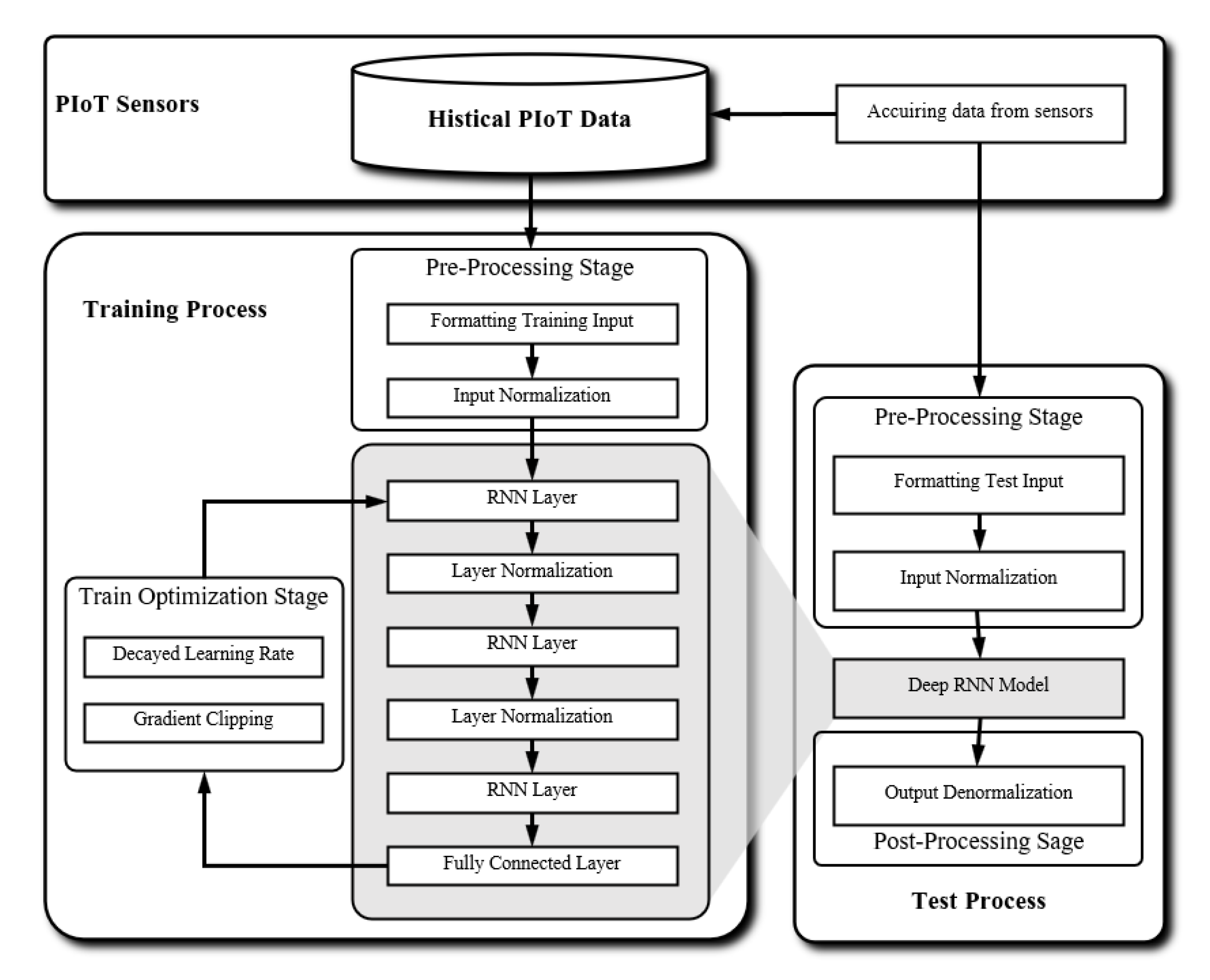
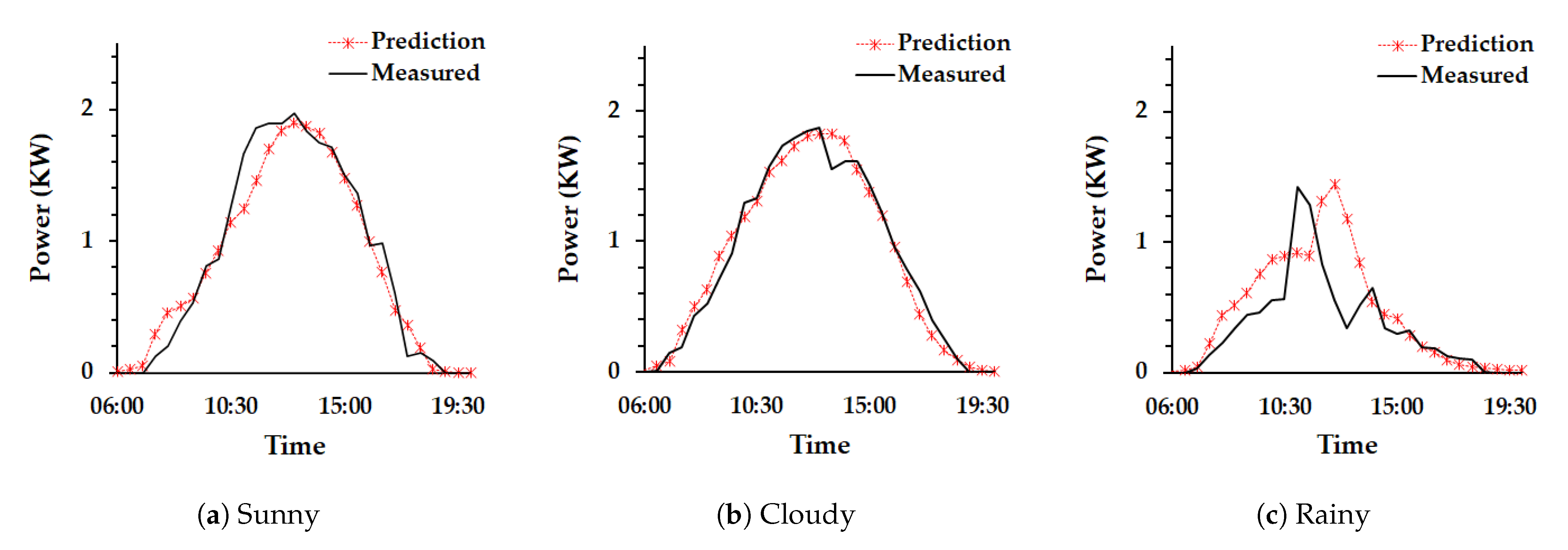
In this paper, we proposed the deep RNN-based short-term forecast algorithm of PV power generation. For the proposed short-term forecast of PV power generation, we collect on-site power and weather information using PIoT sensors installed in a PV power system since on-site accurate weather information is significant for the short-term prediction accuracy. We performed a correlation analysis between the PV generated power data and meteorological data collected in a PV system to select the weather parameters. The correlation analysis confirmed that solar power was affected by solar irradiation, ambient temperature, and module temperature. Furthermore, we found that humidity and wind speed are significant meteorological features to the change of the PV power through experimental investigations. The proposed short-term forecast of PV power generation is designed based on a deep-RNN model using PIoT data. It consists of one input layer, three hidden RNN layers, and one fully connected output layer. The sequence inputs are normalized, and their outputs are denormalized.

To evaluate the performance of short-term forecast PV power, we performed various experiments according to the number of hidden layers, sampling data interval, and the time steps of a deep RNN-based forecast model. Experimental results showed that the prediction accuracy was the best when it consists of 3 hidden RNN layers and 12 time-steps in each RNN layer. In the experiments for the very short-term forecasting algorithm of PV power generation, the prediction accuracy was 99.1% (nMAE)/98.0% (nRMSE) regarding 5 min ahead forecast, and 98.6% (nMAE) 96.6% (nRMSE) regarding 15-min ahead forecast. The R${}^2$-scores of them were 0.988 and 0.949, also. In the experiments for the short-term forecasting algorithm of PV power generation, the prediction accuracy was 94.8% (nRMSE) and 97.4% (nMAE) regarding 1 h ahead forecast and 92.9% (nRMSE) and 96.2% (nMAE) regarding 3 h ahead forecast. The R${}^2$-scores of 1 h and 3 h ahead prediction were 0.963 and 0.927, respectively. Experimental results showed that the proposed deep RNN-based short-term forecast algorithm achieved higher prediction accuracy compared with ARIMA and SVR-RFN models.

To improve the current short-term PV power generation forecast model, we will develop new deep learning forecast models using other weather features like a cloud image and dust sensors in the future. We will study an abnormality detection method in the PV power system based short-term forecast algorithm. We expect that it will be useful for floating or marine photovoltaics.

References

1. IRENA. Renewable Capacity Statistics 2020; International Renewable Energy Agency: Masdar City, UAE, 2020; p. 66. [Google Scholar]
2. Lappalainen, K.; Wang, G.C.; Kleissl, J. Estimation of the largest expected photovoltaic power ramp rates. Appl. Energy 2020, 278, 115636. [Google Scholar] [CrossRef]
3. Bugała, A.; Zaborowicz, M.; Boniecki, P.; Janczak, D.; Koszela, K.; Czekała, W.; Lewicki, A. Short-term forecast of generation of electric energy in photovoltaic systems. Renew. Sustain. Energy Rev. 2018, 81, 306–312. [Google Scholar] [CrossRef]
4. Majidpour, M.; Nazaripouya, H.; Chu, P.; Pota, H.; Gadh, R. Fast Univariate Time Series Prediction of Solar Power for Real-Time Control of Energy Storage System. Forecasting 2019, 1, 107–120. [Google Scholar] [CrossRef] [Green Version]
5. Eltawil, M.A.; Zhao, Z. Grid-connected photovoltaic power systems: Technical and potential problems—A review. Renew. Sustain. Energy Rev. 2010, 14, 112–129. [Google Scholar] [CrossRef]
6. Moreno-Muñoz, A.; De La Rosa, J.J.G.; Posadillo, R.; Pallarés, V. Short term forecasting of solar radiation. In Proceedings of the IEEE International Symposium on Industrial Electronics, Cambridge, UK, 30 June–2 July 2008. [Google Scholar] [CrossRef]
7. Kardakos, E.G.; Alexiadis, M.C.; Vagropoulos, S.I.; Simoglou, C.K.; Biskas, P.N.; Bakirtzis, A.G. Application of time series and artificial neural network models in short-term forecasting of PV power generation. In Proceedings of the Universities Power Engineering Conference, Dublin, Ireland, 2–5 September 2013. [Google Scholar] [CrossRef]
8. Graditi, G.; Ferlito, S.; Adinolfi, G. Comparison of Photovoltaic plant power production prediction methods using a large measured dataset. Renew. Energy 2016, 90, 513–519. [Google Scholar] [CrossRef]
9. Li, Y.; Zhang, J.; Xiao, J.; Tan, Y. Short-term prediction of the output power of PV system based on improved grey prediction model. In Proceedings of the International Conference on Advanced Mechatronic Systems (ICAMechS), Kumamoto, Japan, 10–12 August 2014. [Google Scholar] [CrossRef]
10. Shang, X.X.; Chen, Q.J.; Han, Z.F.; Qian, X.D. Photovoltaic Super-Short Term Power Prediction Based on BP-ANN Generalization Neural Network Technology Research. Adv. Mater. Res. 2013, 791–793, 1925–1928. [Google Scholar] [CrossRef]
11. Al-Amoudi, A.; Zhang, L. Application of radial basis function networks for solar-array modelling and maximum power-point prediction. IEE Proc. Gener. Transm. Distrib. 2002, 147, 310–316. [Google Scholar] [CrossRef]
12. Cervone, G.; Clemente-Harding, L.; Alessandrini, S.; Delle Monache, L. Short-term photovoltaic power forecasting using Artificial Neural Networks and an Analog Ensemble. Renew. Energy 2017, 108, 274–286. [Google Scholar] [CrossRef] [Green Version]
13. Sobri, S.; Koohi-Kamali, S.; Rahim, N.A. Solar photovoltaic generation forecasting methods: A review. Energy Convers. Manag. 2018, 156, 459–497. [Google Scholar] [CrossRef]
14. Wang, J.; Ran, R.; Zhou, Y. A Short-Term Photovoltaic Power Prediction Model Based on an FOS-ELM Algorithm. Appl. Sci. 2017, 7, 423. [Google Scholar] [CrossRef] [Green Version]
15. Eseye, A.T.; Zhang, J.; Zheng, D. Short-term photovoltaic solar power forecasting using a hybrid Wavelet-PSO-SVM model based on SCADA and Meteorological information. Renew. Energy 2018, 118, 357–367. [Google Scholar] [CrossRef]
16. Abdel-Nasser, M.; Mahmoud, K. Accurate photovoltaic power forecasting models using deep LSTM-RNN. Neural Comput. Appl. 2019, 31, 2727–2740. [Google Scholar] [CrossRef]
17. Ospina, J.; Newaz, A.; Omar Faruque, M. Forecasting of PV plant output using hybrid wavelet-based LSTM-DNN structure model. IET Renew. Power Gener. 2019, 13, 1087–1095. [Google Scholar] [CrossRef]
18. Eseye, A.T.; Lehtonen, M.; Tukia, T.; Uimonen, S.; John Millar, R. Adaptive Predictor Subset Selection Strategy for Enhanced Forecasting of Distributed PV Power Generation. IEEE Access 2019, 7, 90652–90665. [Google Scholar] [CrossRef]
19. Sheng, H.; Xiao, J.; Cheng, Y.; Ni, Q.; Wang, S. Short-Term Solar Power Forecasting Based on Weighted Gaussian Process Regression. IEEE Trans. Ind. Electron. 2018, 65, 300–308. [Google Scholar] [CrossRef]
20. Rupnik, B.; Westbrook, O. Ambient temperature correction of photovoltaic system performance data. In Proceedings of the 2014 IEEE 40th Photovoltaic Specialist Conference (PVSC), Denver, CO, USA, 8–13 June 2014. [Google Scholar] [CrossRef]
21. Kim, G.G.; Choi, J.H.; Park, S.Y.; Bhang, B.G.; Nam, W.J.; Cha, H.L.; Park, N.; Ahn, H.K. Prediction Model for PV Performance with Correlation Analysis of Environmental Variables. IEEE J. Photovolt. 2019, 9, 832–841. [Google Scholar] [CrossRef]
22. Choi, J.H.; Hyun, J.H.; Lee, W.; Bhang, B.G.; Min, Y.K.; Ahn, H.K. Power performance of high density photovoltaic module using energy balance model under high humidity environment. Solar Energy 2020. [Google Scholar] [CrossRef]
23. Schwingshackl, C.; Petitta, M.; Wagner, J.E.; Belluardo, G.; Moser, D.; Castelli, M.; Zebisch, M.; Tetzlaff, A. Wind effect on PV module temperature: Analysis of different techniques for an accurate estimation. Energy Procedia 2013, 40, 77–86. [Google Scholar] [CrossRef] [Green Version]
24. Graves, A. Supervised Sequence Labelling with Recurrent Neural Networks; Springer: Berlin/Heidelberg, Germany, 2012. [Google Scholar]
25. Rumelhart, D.E.; Hinton, G.E.; Williams, R.J. Learning representations by back-propagating errors. Nature 1986, 323, 533–536. [Google Scholar] [CrossRef]
26. Hochreiter, S.; Schmidhuber, J. Long short-term memory. Neural Comput. 1997, 9, 1735–1780. [Google Scholar] [CrossRef]
27. Ioffe, S.; Szegedy, C. Batch Normalization: Accelerating Deep Network Training by Reducing Internal Covariate Shift. arXiv 2015, arXiv:1502.03167. [Google Scholar]
28. Ba, J.L.; Kiros, J.R.; Hinton, G.E. Layer Normalization. arXiv 2016, arXiv:1607.06450. [Google Scholar]
29. Diederik, P.K.; Ba, J.L. Adam: A Method for Stochastic Optimization. arXiv 2015, arXiv:1412.6980. [Google Scholar]
30. Das, U.K.; Tey, K.S.; Seyedmahmoudian, M.; Mekhilef, S.; Idris, M.Y.I.; Van Deventer, W.; Horan, B.; Stojcevski, A. Forecasting of photovoltaic power generation and model optimization: A review. Renew. Sustain. Energy Rev. 2018, 81, 912–928. [Google Scholar] [CrossRef]
31. Atique, S.; Noureen, S.; Roy, V.; Subburaj, V.; Bayne, S.; MacFie, J. Forecasting of total daily solar energy generation using ARIMA: A case study. In Proceedings of the 2019 IEEE 9th Annual Computing and Communication Workshop and Conference (CCWC), Las Vegas, NV, USA, 7–9 January 2019. [Google Scholar] [CrossRef]
32. Das, U.K.; Tey, K.S.; Seyedmahmoudian, M.; Idna Idris, M.Y.; Mekhilef, S.; Horan, B.; Stojcevski, A. SVR-based model to forecast PV power generation under differentweather conditions. Energies 2017, 10, 876. [Google Scholar] [CrossRef]
33. Pedregosa, F.; Varoquaux, G.; Gramfort, A.; Michel, V.; Thirion, B.; Grisel, O.; Blondel, M.; Prettenhofer, P.; Weiss, R.; Dubourg, V.; et al. Scikit-learn: Machine Learning in Python. J. Mach. Learn. Res. 2011, 12, 2825–2830. [Google Scholar]
Figure 1. Photovoltaic power generation system with PIoT sensors.
Energies 14 00436 g001
Figure 2. Correlation analysis of PIoT data in the PV system: P (Power), S (Solar Radiation), MT (Module Temperature), AT (Ambient Temperature), H (Humidity), and WS (Wind Speed).
Energies 14 00436 g002
Figure 3. The structure of a recurrent neural network.
Energies 14 00436 g003
Figure 4. The structure of an LSTM cell.
Energies 14 00436 g004
Figure 5. The proposed deep RNN to forecast PV power generation.
Energies 14 00436 g005
Figure 6. The PIoT sensor inputs and output of the deep RNN model to predict PV power generation.
Energies 14 00436 g006
Figure 7. The architecture of Deep-RNN.
Energies 14 00436 g007
Figure 8. PV Power Platform with IoT sensors in Konkuk University.
Energies 14 00436 g008
Figure 9. 5 min ahead very short-term forecast result of PV power generation (Layer = 3).
Energies 14 00436 g009
Figure 10. 15 min very short-term ahead forecast result of PV power generation (Layer = 3).
Energies 14 00436 g010
Figure 11. The very short-term forecast results for 6 consecutive days (RNN layers = 3, time steps = 12).
Energies 14 00436 g011
Figure 12. Scatter graph of the very short-term forecast results (RNN layers = 3, time steps = 12).
Energies 14 00436 g012
Figure 13. The 1 h ahead short-term forecast (SI = 30 m, PDL = 12 h, Layer = 3).
Energies 14 00436 g013
Figure 14. The 3 h ahead short-term forecast (SI = 30 m, PDL = 12 h, Layer = 3).
Energies 14 00436 g014
Figure 15. The short-term forecast results of PV power generation for 6 consecutive days (RNN layers = 3, time steps = 12, sampling interval = 30 min).
Energies 14 00436 g015
Figure 16. Scatter plots of short-term forecast results (RNN layers = 3, time steps = 12, sampling interval = 30 min).
Energies 14 00436 g016