Abstract
Using aerodynamic resistance to provide braking force for trains is an economical braking method. It has few components to wear out and requires no energy. But the aerodynamic braking plate will significantly affect train’s aerodynamics behaviors. This paper studies the effect of the braking plates’ layout on the aerodynamic force of head car when a train is running under a crosswind. The results show that the braking plate will not only increase the drag force, but also significantly affect the lift and lateral force of the train’s head car. The installation position of the braking plates will also have a great effect on the aerodynamic force. In order to increase the drag force and weaken other aerodynamic force changes of the head car, we suggest that the first braking plate be arranged at the end of a streamlined shape, and the second braking plate be arranged at the middle of the car body. Compared with trains without braking plates, the head car’s drag force increases by 85.7%, lift force only increases by 7.6%, and side force decreases by 5.9%, when the braking plates are in operation.
1. Introduction
For trains, the traditional braking methods include friction braking, eddy current braking, and so on. All of the above braking methods require energy consumption and are prone to wear and tear of components. Aerodynamic resistance is an important part of the running resistance of a train, and as the speed increases, the aerodynamic resistance will also increase dramatically [1]. Using aerodynamic resistance to provide braking force has become very promising.
Regarding the aerodynamic braking, Japan and China have conducted experimental studies on the full-scale model and confirmed that the devices can effectively improve the braking performance of the train [2,3,4]. Some scholars have also used numerical methods to study braking plates. Lee and Bhandari [5] studied the resistance characteristics of trains at different train speed levels and different plates’ angles without crosswind. Puharic et al. [6] studied the contribution of braking plates to the total braking force of trains at different speed levels. Wu et al. [7] researched the aerodynamic effects of braking plate during trains passing-by. Gao et al. [8] researched the effect of the angle of the braking plate on the braking force without crosswind. Niu et al. [9,10] studied the mutual influence of braking plates, and believed that the installment position of braking plates was very important. Tian et al. [11] used a simplified train model to study the effect of braking plates on the derailment coefficient. Zhai et al. [12] mainly studied the flow field structure near the braking plate with and without crosswind but paid little attention to the aerodynamic characteristics of trains.
In the past, scholars generally focused on the aerodynamic resistance features of braking plates. But the characteristics of a train under crosswind are very different from those when there is no crosswind. The drag, lift, and side force will change greatly [13,14,15,16,17]. The fact is that the train’s aerodynamic load has a very large influence on the train’s running status, and even affects the train’s safety [18,19,20,21,22,23]. Trains with braking plates are more susceptible to airflow, especially when encountering crosswinds, and their operating safety may deteriorate further. It is necessary to research the effect of the braking plate on the aerodynamic load of the railway vehicles under typical wind speed and find a solution that can not only improve the braking effect of trains, but also reduce the adverse effects of side force and lift force. In combination with the surrogate model method, we explored the effect of installation positions of the two braking plates of the head car on the aerodynamic force and obtained the internal law between the installation position of the braking plates and the aerodynamic force. Then, we obtained a layout with high drag force, low side force, and lift force.
2. Methods
2.1. Fluid Mechanics
For a running train, the surrounding flow field can be described by the Navier-Stokes equation. The generalized governing equation is as follows:
where u is the velocity, P is pressure, ν is the coefficient of kinematic viscosity, and f is the external force.
2.2. Kriging Regression
The surrogate model method is a global optimization method. It mainly expresses the relationship between design variables and output by constructing a function with appropriate accuracy. In this paper, we study the relationship between the position of the braking plate and the drag coefficient, side force coefficient, and lift coefficient of the head car. The positions of the two braking plates are the independent variables of the surrogate model, and the aerodynamic coefficient of the head vehicle is the dependent variable of the surrogate model. Therefore, the position coordinates of the braking plate and the aerodynamic coefficient of the vehicle are the parameters we need to collect. We cannot construct a surrogate model out of thin air. The surrogate model must be based on observed data. These observed data are the sample points in this paper. In other words, the position coordinates of the braking plate of the sample point and the corresponding train’s aerodynamic force are known to us (by computational fluid dynamic simulation). Using some mathematical methods (interpolation or regression), the functional relationship between the position of the braking plate and the aerodynamic force of the train can be obtained based on the data of the existing sample points. The Kriging method is a mathematical method of constructing a surrogate model [24].
The traditional Kriging method is the interpolation method. Given a set of design variables and the observed response values . The purpose of constructing a surrogate model is to make a prediction for an unknown point x based on the existing data. We assume that all observed responses come from a random process Y. The mean value of this random process is 1 μ (1 is an n × 1 order unit column vector):
Responses can be correlated with the following basis function:
where θ is a scale parameter, determined by the genetic algorithm.
According to Equation (4), an order correlation matrix can be established that relates all observation points:
Then, the prediction of the unknown point x by the Kriging model is:
where ψ is the correlation vector of the unknown point x and the known points:
Because simple interpolation does not fit the trend between the sample variables and the outputs well in some cases (it is easy to overfit), we employed the Kriging regression model. The model need not interpolate the sample data. We need to add a regression constant λ on the main diagonal of the correlation matrix [25]. That is, the correlation matrix becomes . (I is identity matrix). After testing, λ = 0.0035 in this paper. Then, the expression of the predicted value of the Kriging regression model is:
3. Numerical Model and Validation
3.1. Numerical Model
The model consists of head and middle car. Li et al. [26] used this model (head car, middle car, and tail car) as the object to research the influence of inter-car clearance extent on the aerodynamic performance of the train. In this paper, our focus is on the head car of the train. In order to ensure the consistency of the boundary conditions of the model, we retain the middle car without braking plates and bogies in the calculation model. The head car is selected because the head car aerodynamic force is not easily affected by the middle car. The model is a 1:8 scaled model, the characteristic height of the car is 0.52 m, and the length of the head car and the middle car are 3.45 and 3.125 m, respectively. The cross-section area of vehicle is 0.1687 m2. We installed two sets of braking plates in the head car. The length, width, and height of each braking plate are 110 × 80 × 8 mm. The angle of the braking plate is 75°. Because this angle is within the encouragement interval, the opening of the braking plate can be aided by wind force [3]. The geometric model of the train, the placements of braking plate, and calculation domain are displayed in Figure 1.
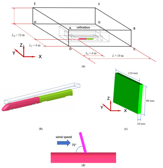
Figure 1.
Calculation model of train: (a) Calculation domain, (b) train model and braking plates, (c) braking plate, and (d) angle of braking plate.
3.2. Simulation Settings
The commercial software Fluent was used to simulate the train’s operation status. Only when the speed is high enough can the braking plate play a greater role. But in actual situations, trains often run at reduced speeds when encountering strong crosswinds. Therefore, the relationship between wind speed and vehicle speed must be weighed when determining the simulated wind speed. The operating speed of current high-speed trains is generally 250 or 300 km/h, and when encountering strong crosswinds, the train speed cannot reach 300 km/h. Therefore, we finally determined that the train speed is 250 km/h, and the wind speed is 15 m/s. The aerodynamics of trains has always been a research hotspot, and many simulation studies on it have been published [14,26,27,28]. Therefore, it can provide references for the selection of related turbulence models and other parameters in this paper. In addition, in the model verification chapter, we have also done a lot of verification to prove the reliability of the simulation. The theory of Fluent software is the finite volume method. Use steady-state mode for simulation. The turbulence model is the k-ω shear stress transport (SST) model. Because, when there are flow separation and reverse pressure gradient phenomena, the prediction performance of this turbulence model is better, . The velocity of the airflow around the train is less than 0.3 times the Mach number, so it can be regarded as an incompressible fluid. We chose the pressure-based solver because it is more suitable for low-pressure or incompressible cases. Using a simple algorithm, momentum, turbulent kinetic energy, and specific dissipation rate are all second-order upwind. In the calculation domain shown in Figure 1a, ABCD and ADHE are velocity inlet, , BCGF and FGHE are pressure outlets, ABFE is a non-slip wall, CDHG is a sliding wall, and sliding speed . The aerodynamic forces in this paper are all expressed in dimensionless form. The definitions of aerodynamic coefficients are as follows:
where , , , and Cp are drag force coefficient, lift force coefficient, side force coefficient, and pressure coefficient. Fd is the drag force, Fl is lift force, Fs is side force, A = 0.1687 m2, ρ = 1.225 kg/m3, is train velocity, and is wind velocity.
3.3. Validation
Since there are currently no publicly available wind tunnel tests’ data conducted on trains with wind brake systems, we adopt a step-by-step verification plan. Firstly, verify whether the simulation method is appropriate, and then perform aerodynamic verification on the train and brake plates separately to determine whether the mesh size is appropriate. Finally, the brake plate is installed on the train to further verify whether the surface pressure of the train caused by the brake plate will be affected by the mesh size.
3.3.1. Simulation Method Verification
The simplified train has been studied by scholars and has detailed surface pressure data [29]. The shape of the simplified train is similar to the shape of the train in this article (both are prismatic structure), and the simulation scene is similar (with crosswind), so it is very suitable for simulation method verification. The simplified train model, the position of the calculation domain, and the loops for extracting the pressure coefficient are shown in Figure 2. The pressure coefficient of each loop is shown in Figure 3.
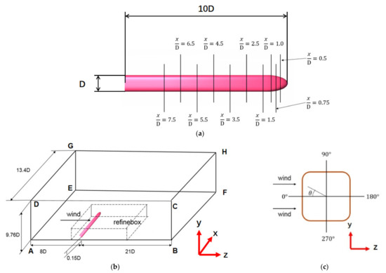
Figure 2.
Calculation model of simplified train: (a) Simplified train, (b) calculation domain, and (c) pressure coefficient angle definition.
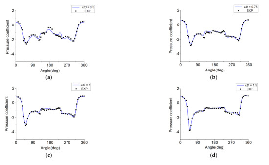
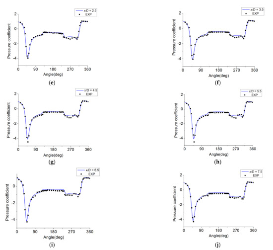
Figure 3.
Pressure coefficient verification of simplified train: (a) Pressure coefficient verification at x/D = 0.50, (b)pressure coefficient verification at x/D = 0.75, (c) pressure coefficient verification at x/D = 1, (d) pressure coefficient verification at x/D = 1.50, (e) pressure coefficient verification at x/D = 2.5, (f) pressure coefficient verification at x/D = 3.5, (g) pressure coefficient verification at x/D = 4.5, (h) pressure coefficient verification at x/D = 5.5, (i) pressure coefficient verification at x/D = 6.5, and (j) pressure coefficient verification at x/D = 7.5.
From the verification results, the simulated value of the model surface pressure coefficient is in good agreement with the experiment, indicating that the simulation method is suitable for this type of problem.
3.3.2. Aerodynamic Verification of Train without Braking Plates
Li et al. [26] have done experiments on the aerodynamics of this model without braking plates in a windless environment. The boundary ADHE of the calculation domain is the velocity inlet, , and BCGF is the pressure outlet. The remaining boundary is set to the wall. The verification is shown in Table 1.

Table 1.
Train aerodynamic verification.
We can see that there is not much difference in the aerodynamic coefficient between EXP and M2 and M3. Since the computational cost is proportional to the number of grids, we choose M2 as the meshing scheme of the train. In addition, we also verified the train aerodynamic forces of different turbulence models (k-epsilon, k-omega, Spalart Almaras) using M2. In order to ensure the consistency of the algorithm, the second-order format is used for spatial discretization. The verification results are shown in Table 2. The k-omega turbulence model still shows advantages.
Table 2.
Train aerodynamic verification.
3.3.3. Flat Plane’s Aerodynamic Verification
The verification of plate aerodynamic force is to verify whether the plate’s grid is reasonable. The drag and lift coefficients of a two-dimensional plate with a large angle of attack can be expressed by the following equations [30]:
where α is the angle of attack.
A two-dimensional flat plate can be regarded as an infinitely long flat plate in three-dimensional space. Therefore, the length, width, and height of the plate we chose are 1, 0.1, and 0.005 m, respectively. The plate model and the computational domain are shown in Figure 4.
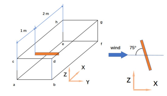
Figure 4.
The calculation domain of the verification model.
In order to increase the length of the plate without increasing the number of grids, the plate is consolidated with the boundary “ache”. The boundary condition of “ache” is set to symmetry. The velocity inlet is “abcd”, velocity is 30 m/s, and “ehgf” is the pressure outlet. Since the angle of the brake plate in this article is 75 degrees, the angle of attack of the plate is also 75 degrees. The verification results are shown in Table 3. The simulated values of aerodynamic coefficient are not much different from the theoretical ones.
Table 3.
Drag force verification of three-dimensional (3D) flat plate.
3.3.4. Overall Verification
Through the above verification, we initially determined the simulation method and the mesh size of each part of the model, and we used this as a benchmark. Now, we install the braking plate on the train and encrypt the grid again to verify whether the surface pressure coefficient of the train with the braking plate is different from the benchmark mesh. We extracted the pressure coefficients of 4 loops, as shown in Figure 5a. Loop 1 is located 0.2 m in front of the first braking plate, loop 2 is located at the midpoint of the two plates, loop 3 is located 0.2 m behind the second braking plate, and loop 4 is located 0.15 m from the rear end of the head car. On each loop, we extract the surface pressure coefficient. The angle of each point on the loop relative to the center of the cross-section is displayed by Figure 5b. The verification result is shown in Figure 6. The results show that the pressure coefficients of the three sets of meshes are very close.
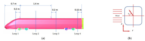
Figure 5.
Location of loops: (a) loops, and (b) pressure coefficient angle definition.
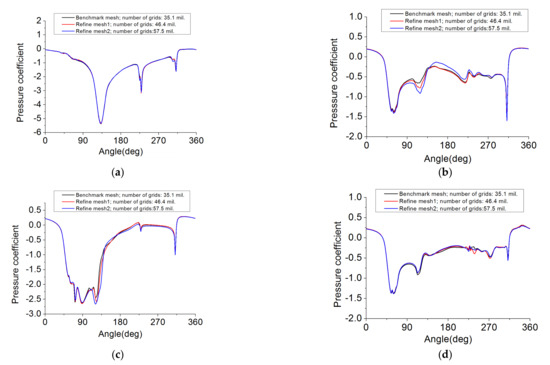
Figure 6.
Pressure coefficient verification of simplified train: (a) Loop 1, (b) loop 2, (c) loop 3, and (d) loop 4.
3.4. Grid Size of Train and Braking Plates
We determined the grid size of the train and braking plates. The surface grid size of the car body is 8 mm, and the braking plates’ grid size is 0.5 mm. The total number of grids is 35.1 million. The number of boundary layers is 12. In order to achieve the maximum potential of the SST model, “y+” had better be less than or equal to 1. “y+” has a great relationship with the height of the first boundary layer, and the height can be roughly estimated by the formula:
where H is the height of the first boundary layer, is the kinematic viscosity of the fluid, and is reference length.
Through calculation, the height of the first boundary layer is 0.01 mm. The growth rate of the last two boundary layers is 1.4 and the rest are 1.2. The boundary layer and y+ of the train are shown in Figure 7.
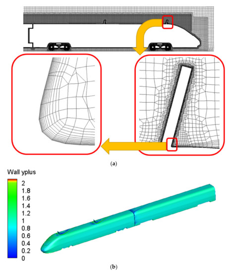
Figure 7.
Model’s grid and y+. (a) Grid and boundary layer of train body and braking plates. (b) y+ of train body and brake plates.
4. Result
4.1. Influence of Installation Position of Braking Plates on the Aerodynamic Loads of the Head Car
In the field of engineering optimization, the surrogate model method is widely used [31,32]. This paper studied the relationship between the position of the braking plates and the aerodynamic loads. Therefore, it requires that the surrogate model must have high accuracy in the entire design space. The design variables are the arrangement positions of the two braking plates: the position of the first plate is , and the position of the second plate is . Two boundaries of the design variables are the end of the streamlined shape and 2.5 m away from the end of the streamlined shape. The range of variables is shown in Figure 8. Two plates are arranged on the two boundaries of the design space, namely . In actual situations, in order to ensure that there is no assembly interference between the braking plates, the distance between the two plates cannot be infinitely short. This paper also limits the minimum distance between two braking plates. The distance between the two braking plates is not less than 0.1 m. Therefore, constraint can be described by inequalities (19)–(21):
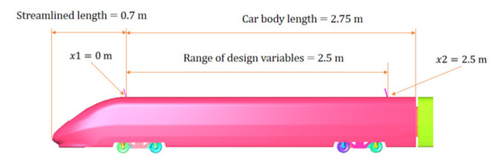
Figure 8.
Range of design variables.
The different arrangements of the braking plates constitute the sample point set. The aerodynamic force (by CFD simulation) of each sample point is used as the response values of the surrogate model. The sample points required by the model are obtained by the Latin hypercube method [33]. Then, the candidate sample points that meet the constraint conditions are selected as the initial samples to construct the surrogate model. The surrogate model built on the initial sample points is often not accurate enough. We need to add points in the follow-up. The follow-up adding point plan mainly consists of two parts. The first part is to explore potential undiscovered areas, so random adding sample points are used. The second part is to encrypt the areas that have been explored. The steps are as follows: Firstly, we used the leave-one-out method [34] to calculate the error between the simulation value of each sample point and the model’s output. Then, the area where the sample point with large error is located is regarded as the key area. The surrogate model needs to add more sample points in this area. By supplementing the sample points many times, the mapping accuracy of the surrogate model has been greatly improved. We have a total of 99 samples. The average error is shown in Table 4. The average error is defined as follows:
where N is 99, is the predicted value of sample i, and is the simulation value of sample i.
Table 4.
Average error of surrogate model.
The average errors of the surrogate model in drag, side, and lift force are less than 3%. From this, we get a surrogate model with global high accuracy. Then, the relationship between the positions of the braking plates and the aerodynamic loads of the head car can be described by the surrogate model, as shown in Figure 9.
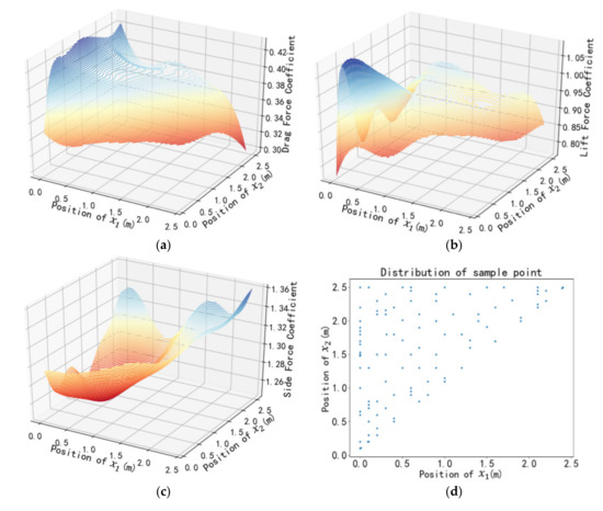
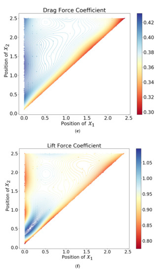
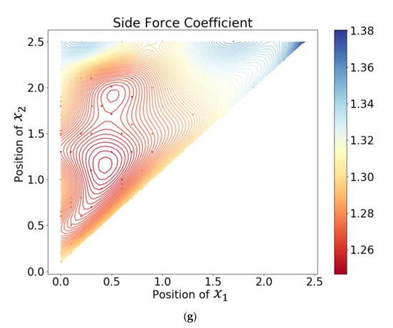
Figure 9.
Relationship between braking plate positions and aerodynamic loads: (a) Relationship between positions and drag force (three-dimensional (3D) format), (b) relationship between positions and lift force (3D format), (c) relationship between positions and side force (3D format), (d) sample points, (e) relationship between positions and drag force (contour format), (f) relationship between positions and lift force (contour format), and (g) relationship between positions and side force (contour format).
Figure 9a–c shows the relationship between the positions of the braking plate and the aerodynamic loads in the form of a three-dimensional (3D) format. Although the three-dimensional image allows us to intuitively understand the shape of the function, it is also difficult to see the full appearance of the function because of the occlusion of the curved surface. Therefore, we supplement Figure 9e–g. The subfigures show the relationship between the positions of the braking plate and the aerodynamic load in the form of a contour map and use color to indicate the amplitude of the aerodynamic load. The denser the contour lines’ distribution, the more drastic the aerodynamic load changes in this area. The points in Figure 9e–g are the sample points of the surrogate model. We observed that the color difference between most of sample points and the contour lines is so small that some points are even difficult to identify. This also indicates that the mapping precision of the surrogate model is high. The specific distribution of sample points is shown in Figure 9d. The entire design space is a triangle in the coordinate system because of the constraint of inequality (21). The sample points are located inside or on the boundary of this triangle. From a global perspective, the average differences between the drag, side force, and lift coefficients by the Kriging model and the CFD simulation are 2.474%, 2.944%, and 0.791%, respectively. Therefore, the global accuracy of the Kriging method used in this article is relatively high. But, considering that CFD simulation will have errors compared with experimental values, the surrogate model is constructed based on simulation values, so there will inevitably be a superposition of errors. Therefore, we should pay more attention to areas with obvious trends shown by the model, such as extreme areas, because these areas show strong consistency in both simulation value and model output values. In addition, the extreme value areas are also areas of more concern in engineering.
Combining Figure 9a,e, we see that the drag coefficient presents a trend of changing from high left to low right and flat in the middle in the design space. We roughly divide it into three areas, namely high-drag area, middle-drag aera, and low-drag area. The high-drag area is at the far left of the design space, that is, when the first braking plate is near (end of streamlined shape). In this area, as long as the second braking plate is not very close to the first plate, the vehicle can obtain a larger drag force. This shows that the position of the first braking plate has a great effect on resistance. The color of the low-drag area is red. The low-drag area is at the right end of the design space. In this area, the position of the first braking plate is very close to the second braking plate. This means that the braking plates cannot be too close together, and being too close will affect each other, reducing the drag performance. The middle-drag area is located between the two areas. The color of the contour line in this area is light blue, and the distribution of the contour lines is relatively sparse. It shows that the change of drag force in this area is not obvious. When the first braking plate is not near the end of the streamlined shape and it is also aloof from the second plate, the position of the braking plate has little effect on the drag force.
Figure 9b,f shows the relationship between the positions of the braking plate and the lift force. We noticed that in a specific area, the function is shaped like a very steep mountain. The steeper the mountain, the greater the lift force. We call this area a mountain area. Lift force will deteriorate the safety of the train, so we do not recommend placing braking plates in this area. We noticed that the mountain area is in the lower left corner of the design space. This shows that when both the first and the second braking plates are arranged at the forepart of the car body, the lift force will be greatly increased. We noticed that there is a part of overlap between the mountain area of lift force and the high drag area, but the area of overlap is not large. In addition, we also found two areas with less lift force. One of them completely coincides with the low-drag area. That is, when the two braking plates are very close, the lift force is small. Another area is also near . When the first braking plate is located at the end of the streamlined shape and the second braking plate is not close to the car’s head, head car’s resistance is large, and the lift force is small.
Figure 9c,g shows the relationship between the positions of the braking plate and the side force. The function is shaped like a basin. The contour line of the bottom of the basin is relatively sparse, indicating that the bottom is flat. The high value area of side force is basically distributed at the top of the design space, that is, when the position of the second plate is located at the rear of the vehicle body, it is possible to increase the side force. Excessive side force will also affect the safety of the train. From this, we can get a series of engineering conclusions: Firstly, the two braking plates cannot be arranged very close together. Although the closer distance can reduce the lift increase, it will also suppress the drag force increase. Secondly, when the first braking plate is placed at the end of the streamlined shape, the head car can obtain greater drag force. However, the two braking plates cannot be near the car’s head all at once, otherwise the lift force will be increased a lot. Thirdly, the second braking plate cannot be placed at the rear of the car body, otherwise head car’s side force may be increased. Under crosswind, the best arrangement is that the first plate is arranged at the end of the streamlined shape, and the second plate is arranged at the middle of the car body.
4.2. Comparison in Aerodynamic Characteristics
In combination with the conclusion of Section 4.1, we selected the head car with the braking plate position to compare with the head car without braking plates, as shown in Table 5. The drag force increased by 85.7%, the lift force increased by only 7.6%, and the side force decreased by 5.9%. We made the slice and loops as shown in Figure 10 to analyze the differences between the two models. The slice is located at the symmetry axis of the train. The comparison result is shown in Figure 11.
Table 5.
Aerodynamic coefficients of the two models.
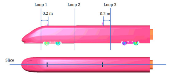
Figure 10.
Location of slice and loops.
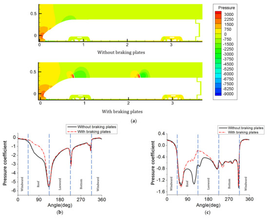
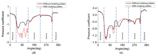
Figure 11.
Comparison of aerodynamic characteristics of the two models. (a) Pressure comparison slice between two models (Pa), (b) pressure coefficient comparison of loop 1, (c) pressure coefficient comparison of loop 2, (d) pressure coefficient comparison of loop 3, and (e) pressure coefficient comparison of loop 4.
Figure 11a is the pressure distribution slice of the two models. We noticed that the two models have obvious differences in pressure distribution. The model without a braking plate shows a clear zone of negative pressure at the end of the streamline shape. In the model with braking plates, this negative pressure zone is destroyed by the braking plate. The streamlined part of the original model’s head car is an arc structure, and the negative pressure area at the top of the streamlined shape will weaken the resistance of the train. Placing a brake plate on the end of the streamlined shape not only allows the brake plate to obtain resistance gain, but the streamlined shape can also obtain a certain resistance gain. At the front of the two braking plates, obvious positive pressure zones appeared. At the rear of the braking plates, obvious negative pressure zones appeared accordingly. This is led by the blocking effect of the braking plate. Because there is no other braking plate in front of the first braking plate to disturb the flow field, the airflow impact on the first braking plate is greater than that of the second brake plate, which causes the negative pressure area behind the first brake plate to be more severe. The front of the braking plate is positive pressure, and the rear of the brake plate is negative pressure. This pressure distribution does bring additional resistance to the running train. The pressure change on the roof will also influence the lift force. So, the two models will be different in side and lift force. The biggest difference of loop 1 is at the top. The negative pressure coefficient of the train without braking plates is larger than that of the train with braking plates. This means that the braking plate will weaken the upward lift force in this area.
The biggest difference in loop 2 is at the upper side and the leeward of the head car. We noticed that the coefficient of the train without braking plates is larger than the train with braking plates. This shows that the braking plates can also weaken the lift and side forces in this area.
The biggest difference in loop 3 is at the roof of the head car. Different from the first two loops, the negative pressure coefficient at the upper side of the vehicle with braking plates is larger than the train without plates. This is due to the blocking effect of the braking plates causing eddies to appear at the rear of the plate [9,10].
The biggest difference in loop 4 is at the upper and leeward side of the vehicle. The coefficient of the vehicle with braking plates is larger than the model without braking plates. On the leeward side, the negative pressure coefficients of the two models are also different at different angles.
According to the data of each loop, the pressure coefficients of the two models differ greatly at the top and the leeward side. The pressure coefficients at the bottom of the two models are not very different. On the windward side, the pressure coefficients of the two models are almost the same. This shows that the top and the leeward side of the train are more susceptible to braking plates. This is the result of the combined action of the braking plate and the crosswind. When the train is running, the fluid turbulence behind the braking plate becomes stronger, and the effect of the crosswind will bring the influence of the turbulence to the leeward side of the train.
5. Conclusions
By studying the influence of the angle and placement of the braking plates on aerodynamic force of the train under the crosswind, the following conclusions can be obtained:
- The braking plate will not only change the drag force, but also significantly change the side and lift force when the train is running under a crosswind. Therefore, the influence of the braking plate on the aerodynamic force of the train should also be taken into account when designing and arranging it.
- The installation positions of the braking plate will also significantly affect the aerodynamic force of the head car. When the positions of the two braking plates are very close to each other, the drag increase will be suppressed. When the first braking plate is located near the end of the streamlined shape, the drag force of the head car is often relatively large, but if both braking plates are close to the car’s head, the lift force may increase. When the second plate is located at the rear of the vehicle body, the side force may increase. Therefore, we recommend that the first braking plate be placed at the end of the streamlined shape, and the second braking plate be placed at the middle of the car body.
- The braking plate has a huge influence on the pressure coefficient of the leeward side and the upper side of the head car, especially the upper side. The braking plate has little effect on the pressure coefficient at the bottom of the train and has almost no effect on the windward side.
Author Contributions
Conceptualization, L.Z. and T.L.; methodology, L.Z. and J.Z.; software, L.Z.; validation, L.Z. and T.L. writing, L.Z. All authors have read and agreed to the published version of the manuscript.
Funding
This project was supported by The National Key Research and Development Program of China (2020YFA0710902), China Postdoctoral Science Foundation (No. 2019M663550) and Self-determined Project of State Key Laboratory of Traction Power (2019TPL_T02).
Institutional Review Board Statement
Not applicable.
Informed Consent Statement
Not applicable.
Data Availability Statement
The raw/processed data required to reproduce these findings cannot be shared at this time as the data also forms part of an ongoing study.
Conflicts of Interest
The authors declare no conflict of interest.
References
- Tian, H. Review of research on high-speed railway aerodynamics in China. Trans. Saf. Environ. 2019, 1, 1–21. [Google Scholar]
- Sawada, K. Development of magnetically levitated high speed transport system in Japan. IEEE Trans. Magn. 1996, 32, 2230–2235. [Google Scholar] [CrossRef]
- Yoshimura, M.; Saito, S.; Hosaka, S.; Tsunoda, H. Characteristics of the aerodynamic brake of the vehicle on the Yamanashi Maglev test line. Q. Rep. RTRI 2000, 41, 74–78. [Google Scholar] [CrossRef]
- Zuo, J.Y.; Wu, M.L.; Tian, C. Aerodynamic braking device for high-speed trains: Design, simulation and experiment. Proc. Inst. Mech. Eng. Part F J. Rail Rapid Transit 2014, 228, 260–270. [Google Scholar]
- Lee, M.; Bhandari, B. The application of aerodynamic brake for high-speed trains. J. Mech. Sci. Technol. 2018, 32, 5749–5754. [Google Scholar] [CrossRef]
- Puharić, M.; Matić, D.; Linić, S.; Ristic, S.; Lucanin, V. Determination of braking force on the aerodynamic brake by numerical simulations. FME Trans. 2014, 42, 106–111. [Google Scholar] [CrossRef]
- Wu, M.L.; Zhu, Y.Y.; Tian, C.; Fei, W.W. Influence of aerodynamic braking on the pressure wave of a crossing high-speed train. J. Zhejiang Univ. Sci. A 2011, 12, 979–984. [Google Scholar] [CrossRef]
- Gao, L.; Xi, Y.; Wang, G.; Wang, G.; Zhang, P.; Zuo, J. Opening Angle rules of the Aerodynamic Brake Panel. J. Donghua Univ. 2016, 33, 20–24. [Google Scholar]
- Niu, J.Q.; Wang, Y.M.; Wu, D.; Liu, F. Comparison of different configurations of aerodynamic braking plate on the flow around a high-speed train. Eng. Appl. Comp. Fluid Mech. 2020, 14, 655–668. [Google Scholar] [CrossRef]
- Niu, J.Q.; Wang, Y.M.; Liu, F.; Chen, Z. Comparative study on the effect of aerodynamic braking plates mounted at the inter-carriage region of a high-speed train with pantograph and air-conditioning unit for enhanced braking. J. Wind Eng. Ind. Aerodyn. 2020, 206, 104360. [Google Scholar] [CrossRef]
- Tian, C.; Wu, M.L.; Zhu, Y.Y.; Chen, M.T. Running Safety of High-speed Train Equipped with Aerodynamic Brake under Cross Wind. In Proceedings of the 2nd International Conference on Energy, Environment and Sustainable Development, Jilin, China, 12–14 October 2012. [Google Scholar]
- Zhai, Y.J.; Niu, J.Q.; Wang, Y.M. Unsteady flow and aerodynamic behavior of high-speed train braking plates with and without crosswinds. J. Wind Eng. Ind. Aerodyn. 2020, 206, 104309. [Google Scholar] [CrossRef]
- Chen, Z.W.; Liu, T.H.; Yan, C.G.; Yu, M.; Guo, Z.J.; Wang, T.T. Numerical simulation and comparison of the slipstreams of trains with different nose lengths under crosswind. J. Wind Eng. Ind. Aerodyn. 2019, 190, 256–272. [Google Scholar]
- Munoz-Paniagua, J.; Garcia, J.; Lehugeur, B. Evaluation of RANS, SAS and IDDES models for the simulation of the flow around a high-speed train subjected to crosswind. J. Wind Eng. Ind. Aerodyn. 2017, 171, 50–66. [Google Scholar]
- Zhang, J.; He, K.; Xiong, X.; Wang, J.; Gao, G. Numerical Simulation with a DES Approach for a High-Speed Train Subjected to the Crosswind. J. Appl. Fluid Mech. 2017, 10, 1329–1342. [Google Scholar]
- Premoli, A.; Rocchi, D.; Schito, P.; Tomasini, G. Comparison between steady and moving railway vehicles subjected to crosswind by CFD analysis. J. Wind Eng. Ind. Aerodyn. 2016, 156, 29–40. [Google Scholar]
- Guo, Z.J.; Liu, T.H.; Yu, M.; Chen, Z.; Li, W.; Huo, X.; Liu, H. Numerical study for the aerodynamic performance of double unit train under crosswind. J. Wind Eng. Ind. Aerodyn. 2019, 191, 203–214. [Google Scholar] [CrossRef]
- Liu, D.R.; Wang, T.T.; Liang, X.F.; Meng, S.; Zhong, M.; Lu, Z. High-speed train overturning safety under varying wind speed conditions. J. Wind Eng. Ind. Aerodyn. 2020, 198, 104111. [Google Scholar] [CrossRef]
- Yang, W.C.; Deng, E.; Zhu, Z.H.; Lei, M.; Shi, C.; He, H. Sudden Variation Effect of Aerodynamic Loads and Safety Analysis of Running Trains When Entering Tunnel under Crosswind. Appl. Sci. 2020, 10, 1445. [Google Scholar]
- Montenegro, P.A.; Calcada, R.; Carvalho, H. Stability of a train running over the Volga river high-speed railway bridge during crosswinds. Struct. Infrastruct. Eng. 2020, 16, 1121–1137. [Google Scholar]
- Yang, W.C.; Deng, E.; Lei, M.F.; Zhu, Z.H.; Zhang, P.P. Transient aerodynamic performance of high-speed trains when passing through two windproof facilities under crosswinds: A comparative study. Eng. Struct. 2019, 188, 729–744. [Google Scholar]
- Liu, T.H.; Chen, Z.W.; Zhou, X.S.; Zhang, J. A CFD analysis of the aerodynamics of a high-speed train passing through a windbreak transition under crosswind. Eng. Appl. Comp. Fluid Mech. 2018, 12, 137–151. [Google Scholar] [CrossRef]
- Noguchi, Y.; Suzuki, M.; Baker, C.; Nakade, K. Numerical and experimental study on the aerodynamic force coefficients of railway vehicles on an embankment in crosswind. J. Wind Eng. Ind. Aerodyn. 2019, 184, 90–105. [Google Scholar] [CrossRef]
- Jones, D.R.; Schonlau, M.; Welch, W.J. Efficient Global Optimization of Expensive Black-Box Functions. J. Glob. Optim. 1998, 13, 455–492. [Google Scholar] [CrossRef]
- Hoer, A.E.; Kennard, R.W. Ridge Regression: Biased Estimation for Nonorthogonal Problems. Technometrics 2000, 42, 80–86. [Google Scholar] [CrossRef]
- Li, T.; Li, M.; Wang, Z.; Zhang, J. Effect of the inter-car gap length on the aerodynamic characteristics of a high-speed train. Proc. Inst. Mech. Eng. Part F J. Rail Rapid Transit 2019, 233, 448–465. [Google Scholar] [CrossRef]
- Li, T.; Hemida, H.; Zhang, J.Y.; Rashidi, M.; Flynn, D. Comparisons of shear stress transport and detached eddy simulations of the flow around trains. J. Fluid Eng. 2018, 140, 111108. [Google Scholar] [CrossRef]
- García, J.; Crespo, A.; Berasarte, A.; Goikoetxea, J. Study of the flow between the train underbody and the ballast track. J. Wind Eng. Ind. Aerodyn. 2011, 99, 90–105. [Google Scholar] [CrossRef]
- Chiu, T.W.; Squire, L.C. An experimental-study of the flow over a train in a crosswind at large yaw angles up to 90-degress. J. Wind Eng. Ind. Aerodyn. 1992, 45, 47–74. [Google Scholar] [CrossRef]
- Jiang, H.B.; Li, Y.R.; Cheng, Z.Q. Relations of lift and drag coefficients of flow around flat plate. In Proceedings of the International Conference on Experimental and Applied Mechanics, Miami, FL, USA, 20–21 January 2014. [Google Scholar] [CrossRef]
- Munoz-Paniagua, J.; García, J. Aerodynamic surrogate-based optimization of the nose shape of a high-speed train for crosswind and passing-by scenarios. J. Wind Eng. Ind. Aerodyn. 2019, 187, 139–152. [Google Scholar] [CrossRef]
- Montoya, M.C.; Nieto, F.; Hernandez, S.; Kusano, I.; Álvarez, A.J.; Jurado, J.Á. CFD-based aeroelastic characterization of streamlined bridge deck cross-sections subject to shape modifications using surrogate models. J. Wind Eng. Ind. Aerodyn. 2018, 177, 405–428. [Google Scholar] [CrossRef]
- Helton, J.C.; Davis, F.J. Latin hypercube sampling and the propagation of uncertainty in analyses of complex systems. Reliab. Eng. Syst. Saf. 2003, 81, 23–69. [Google Scholar] [CrossRef]
- Vehtari, A.; Gelman, A.; Gabry, J. Practical Bayesian model evaluation using leave-one-out cross-validation and WAIC. Stat. Comput. 2017, 2, 1413–1432. [Google Scholar] [CrossRef]


Publisher’s Note: MDPI stays neutral with regard to jurisdictional claims in published maps and institutional affiliations. |
© 2021 by the authors. Licensee MDPI, Basel, Switzerland. This article is an open access article distributed under the terms and conditions of the Creative Commons Attribution (CC BY) license (http://creativecommons.org/licenses/by/4.0/).