Quantitative Analysis of Degradation Modes of Lithium-Ion Battery under Different Operating Conditions

Abstract

The degradation mode is of great significance for reducing the complexity of research on the aging mechanisms of lithium-ion batteries. Previous studies have grouped the aging mechanisms into three degradation modes: conductivity loss (CL), loss of lithium inventory (LLI) and loss of active material (LAM). Combined with electrochemical impedance spectroscopy (EIS), degradation modes can be identified and quantified non-destructively. This paper aims to extend the application of this method to more operating conditions and explore the impact of external factors on the quantitative results. Here, we design a quantification method using two equivalent circuit models to cope with the different trends of impedance spectra during the aging process. Under four conditions, the changing trends of the quantitative values of the three degradation modes are explored and the effects of the state of charge (SoC) and excitation current during EIS measurement are statistically analyzed. It is verified by experiments that LLI and LAM are the most critical aging mechanisms under various conditions. The selection of SoC has a significant effect on the quantitative results, but the influence of the excitation current is not obvious.

1. Introduction

To cope with the energy crisis and increasingly prominent environmental issues, research and development of electric vehicles has become an important trend [1]. Compared with other types of batteries, lithium-ion batteries have been widely used in electric vehicles because of their higher energy density and longer cycle life [2]. Some advanced post-lithium batteries will have a wider perspective application after the improvement of safety issues and cycle stability [3]. In the field of lithium-ion battery research, the study of the aging mechanism has always been regarded as an essential subject, which has great significance for the trend analysis of power and capacity degradation as well as the prediction of remaining useful life [4]. Finding out the change in the aging process will help guide the rational use of lithium-ion batteries in electric vehicles and prolong battery life.

There are many types of aging mechanisms of lithium-ion batteries, and the interactions between them are very complicated. Researchers are looking for entry points to study the aging mechanism. The impacts of specific aging mechanisms on batteries have been widely studied. Braithwaite et al. [5] analyzed the aging phenomenon of the current-collector in lithium-ion batteries and studied the effects of current-collector wear and peeling on the capacity and impedance of lithium-ion batteries. Christensen et al. [6] focused on the potential failure mechanism caused by particle fracture and electronic isolation of active electrode material in lithium-ion batteries and built a mathematical model to quantify the influence of lithium insertion and extraction. Petzl et al. [7] analyzed the effect of lithium deposition on lithium-ion batteries and the manifestation of lithium deposition at low temperatures. These studies on specific aging mechanisms have provided insight into the diversified analysis of the aging phenomenon in lithium-ion batteries. However, their application is limited due to the lack of a comprehensive review of the aging characteristics.

To address this limitation, some researchers have turned to classify primary aging mechanisms. Christensen et al. [8] partitioned all the aging mechanisms of lithium-ion batteries into two modes: the loss of lithium inventory (LLI) and the loss of active material (LAM). Dubarry et al. [9] built a mechanistic model that can synthesize a variety of aging scenarios mainly based on these two modes. Pastor-Fernández et al. [10] supplemented a degradation mode of conductivity loss (CL) to describe the increase of the ohmic resistance due to degradation in electrode contact or electrolyte conduction. The representative aging mechanisms included in the three degradation modes are summarized in

Table 1. The representative aging mechanisms included in the three degradation modes.

Degradation Mode	Representative Aging Mechanism
CL	Damage of current collectors, peeling and degradation of binder [11].
LLI	Formation, growth and degradation of solid electrolyte interface (SEI) [12,13], electrolyte decomposition [14], lithium plating [15].
LAM	Physical damage [16], chemical reaction decomposition [17], contact isolation [6].

. Compared with the direct study on the aging mechanisms, analyzing the aging process from the perspective of degradation modes significantly reduced the research complexity.

Schindler [18], Zhu [19], and Pastor-Fernández [10,20], among others, inherited the concept of degradation mode and further studied the methods of identifying and quantifying different degradation modes. Schindler et al. [18] built a model-based framework for analysis of degradation pathways and realized the aging contributions separation from LLI and LAM. However, Schindler’s approach relies on destructive half-cell experiments to determine initial electrode balancing, which is inconvenient to implement. Non-destructive methods include incremental capacity analysis (ICA), differential voltage analysis (DVA) and electrochemical impedance spectroscopy (EIS). Zhu et al. [19] combined quantification method using DVA and EIS with post-mortem analysis to enhance the analysis of the aging mechanisms. Pastor-Fernández et al. [20] made a comparison of quantitative results between EIS and incremental capacity-differential voltage (IC-DV) and concluded that the EIS method offer a better resolution of the degradation modes. Combined with the onboard EIS measurement system proposed in [21,22,23], this method is also suitable for real-time quantitative analysis of degradation modes.

Pastor-Fernández et al. [10] established the corresponding relationship between the resistances change of a type of second-order equivalent circuit model and each degradation mode (CL, LLI and LAM), which provided an important idea for identifying and quantifying aging mechanisms using the EIS method. To enhance the application value of this method in more scenarios, we can make improvements on three points. The first point is that only one set of battery cycle life tests is carried out, which leads to a lack of experimental data under different conditions for comparative analysis. The second point is that selecting a single second-order equivalent circuit model cannot guarantee the acquisition of circuit component values consistent with the aging mechanisms. It is necessary to select appropriate equivalent circuit models for different characteristics of EIS and analyze the applicability. The last point is that the EIS measurement may be affected by various external factors such as state of charge (SoC) and alternating current (AC) excitation amplitude. The impact of these external factors on quantitative analysis of degradation modes needs to be further studied.

To achieve these three improvements, this paper designs four sets of battery cycle life tests and conducts a quantitative analysis of the degradation mode using two types of equivalent circuit model under different operating conditions. The rest of the article is presented as follows. Section 2 introduces the battery cycle life test matrix and the EIS measuring process. Section 3 presents methods for quantification of degradation modes under different conditions. Section 4 discusses the quantitative results under different conditions and the effect of SoC and excitation current. Finally, the main findings are summarized in Section 5.

2. Experimental

Cycle life tests and EIS measurements under different operating conditions were carried out to study the change of resistance values and analyze the corresponding degradation modes of lithium-ion batteries.

The test samples are commercial 2.75 Ah nickel-cobalt-aluminum (NCA) lithium-ion batteries with the graphite anode (Samsung INR18650-29E). Experiments were performed on the platform consisting of a Chroma Battery Testing System for battery charge and discharge, a BA500-50 Battery Analyzer for EIS measurement, a thermal chamber for ambient temperature stabilization and a host computer for data sampling.

2.1. Battery Cycle Life Test Matrix

To compare the difference between degradation modes at normal temperature and high temperature and analyze the effects of charging current rates, we designed the experimental matrix recorded in

Table 2. Cycle life experimental matrix of NCA lithium-ion batteries under different conditions.

Group Number	Temperature (${}^{°}$C)	Rate (Charge-Discharge)	Code Name
1#	25	1–1 C	25 ${}^{°}$C@1–1 C
2#	25	0.5–1 C	25 ${}^{°}$[email protected]–1 C
3#	45	1–1 C	45 ${}^{°}$C@1–1 C
4#	45	0.5–1 C	45 ${}^{°}$[email protected]–1 C

. The cycle life test scheme is the constant current (CC) charge and CC discharge. In the tests, the operating voltage ranged from 2.5 to 4.2 V, and the discharging current rate was set as 1 C (C is a unit of charge and discharge rate, equivalent to 2.75 A in this paper) to achieve a balance between the experiment time and the effects of discharging process on battery degradation.

2.2. EIS Measuring Process

The EIS measurements were taken every 50 cycles under each condition. Before the measurement, the tested battery was fully charged and then discharged to the three SoC points of 80%, 50% and 20% in turn. At each SoC, the battery was left to stand for 3 h to eliminate interference from polarization effects. During the entire process of SoC adjustment and EIS measurement, the battery was kept at an ambient temperature of 25 ${}^{°}$C.

The internal resistance of the battery to be tested is about 20 m$\mathrm{\Omega }$. Referring to Huet’s research on EIS [24], the applied voltage amplitude should be around 10 mV to ensure that the impedance measurement is performed under linear conditions. Thus, the impedance spectrum is relatively ideal when an AC stimulus with an amplitude (root mean square) of 500 mA is applied. To explore the influence of the AC excitation amplitude on the EIS measurement results, we set three amplitude conditions of 300, 500 and 800 mA in the experiment. The complete EIS measuring process of lithium batteries under each specific condition is shown in Figure 1.

After 250 cycles of life test under 45 ${}^{°}$[email protected]–1 C condition, the impedance spectrum obtained at 20% SoC with 500 mA excitation is plotted in Figure 2. The AC impedance sampling frequency was set from 10,000 to 0.02 Hz to obtain impedance characteristics from high frequency to low frequency. According to the frequency change, the impedance spectrum can be divided into ultra-high frequencies, high frequencies, mid frequencies and low frequencies. Two separate semi-circles mainly characterize the high-frequency region and the mid-frequency region. The impedance spectrum presented in this shape is typical but not suitable for all conditions. The impedance spectra of all four experimental groups obtained at 20% SoC with 500 mA excitation are shown in Figure 3.

When it is not far from the initial state, only one semi-circle can be clearly identified from the impedance spectrum of each experimental group. As the aging process progresses, all groups show two separate semi-circles except for the group under 25 ${}^{°}$C@1–1 C condition shown in Figure 3a. We obtained similar results under other EIS measurement conditions. This experimental phenomenon indicates that the impedance spectrum of the lithium-ion battery may show two changes under different operating conditions. One is that the impedance curve always maintains the shape with one semi-circle. The other is that the impedance curve gradually separates into two distinguishable semi-circles in the medium-high frequency region. Before establishing the quantification method of degradation modes under different conditions, it is necessary to consider the two types of curve shape comprehensively.

3. Quantification of Degradation Mode

3.1. Quantification Method Based on the Second-Order Equivalent Circuit Model

For impedance curves with two semi-circles, it is appropriate to use the second-order equivalent circuit model shown in Figure 4 for fitting [25,26]. This model is divided into four parts, which is fully corresponding to the frequency division in the impedance spectrum shown in Figure 2. The resistances in this model are associated with some electrochemical phenomena and can be used as indicators for evaluating the state of health (SoH) [27,28]. After simplification, an approximate correspondence between various degradation modes and resistances can be established [10].

The ultra-high frequency band is represented by an inductive structure including two components: an inductance L and an ohmic resistance $R_{\mathrm{ohm}}$. L is a lumped inductance for the stray inductance introduced by the current collector and leads. $R_{\mathrm{ohm}}$ explains the voltage drops from the current collector, binder, electrode and electrolyte electronic particles, all of which are representatives of CL.

In the high-frequency band characterized by the SEI structure, an SEI layer resistance called $R_{\mathrm{sei}}$ is connected with a constant phase element (CPE) called $CP{E}_{\mathrm{sei}}$ in parallel. The formation of SEI between the negative electrode and the electrolyte hinders the transfer of lithium ions between the positive and negative electrodes. Furthermore, the quantity of intercalated and deintercalated lithium ions during the charging and discharging process is reduced [29]. Therefore, $R_{\mathrm{sei}}$ is closely related to LLI. $CP{E}_{\mathrm{sei}}$ is employed to represent the film capacitance considering the dispersion effect.

The charge transfer resistance $R_{\mathrm{ct}}$ on behalf of the medium-frequency band and the Warburg element $Z_{\mathrm{w}}$ on behalf of the low-frequency band are connected in series in the model. Both of them are connected in parallel with a CPE called $CP{E}_{\mathrm{dl}}$, representing a capacitor-like effect called double-layer during charge accumulation progress. $R_{\mathrm{ct}}$ is another important representative of LLI. The irreversible loss of lithium ions reduces the lithium-ion concentration for chemical reactions, making the charge transfer process more difficult [20,28]. $Z_{\mathrm{w}}$ stands for the diffusion impedance of lithium ions in the electrode solid particles, and its real part is called Warburg resistance $R_{\mathrm{w}}$. The diffusion phenomenon describes the motion of charged and uncharged particles (mass transport) to balance concentration differences produced by the change in the electrochemical potential. Besides, the concentration difference is mainly affected by structural transformations of active materials [10]. Thus, $R_{\mathrm{w}}$ can be used to characterize LAM.

To facilitate the impedance fitting work, we set up this model in the commercial ZView Version 3.5f (Scribner Associates, Inc., Southern Pines, NC, USA) software. We fitted the impedance spectrum in the frequency range of 0.02–2000 Hz. Based on the initial value of each resistance estimated through the module fitting function, we obtained further adjusted and optimized fitting results through the overall fitting function. Taking the impedance fitting work of the impedance spectrum shown in Figure 2 as an example, we obtained the fitted curve shown in Figure 5. The fitted curve captures the feature of two semi-circles in the impedance spectrum well, and the sum of square errors (SSE) is 0.0062.

The impedance fitting results under 45 ${}^{°}$[email protected]–1 C condition obtained at 20% SoC with 500 mA excitation are plotted in Figure 6. During the aging process, $R_{\mathrm{ct}}$ and $R_{\mathrm{w}}$ show a clear increasing trend, and $R_{\mathrm{ohm}}$ also rises by a lower rate. Their changes are consistent with the corresponding aging mechanisms. Meanwhile, $R_{\mathrm{sei}}$ floats around 10 m$\mathrm{\Omega }$, which is related to the complex mechanism of the SEI layer. Although the SEI film usually grows and thickens as the battery is aged, the original composition of the film may change to a new composition with higher ionic conductivity, causing $R_{\mathrm{sei}}$ to decrease instead [28,30]. In general, the little SSE of the impedance spectrum fitting and the regular change trend of the resistance values jointly indicate the reasonableness of the second-order model for fitting curve contains two semi-circles.

After obtaining each resistance value in the aging stage, the degradation modes can be quantified by the relative change of its associated resistances. Combined with the mechanism analysis conducted earlier in this section, we use $R_{\mathrm{ohm}}$ to represent CL, $R_{\mathrm{sei}}$ and $R_{\mathrm{ct}}$ to jointly represent LLI and $R_{\mathrm{w}}$ to represent LAM. Admittedly, the aging mechanisms contained in each degradation mode cannot be fully expressed by the resistances representing them. Besides the relevance of the mechanism, the rationality and validity of this simplified correspondence relationship was further proved by comparing the quantitative results obtained with EIS and IC-DV technique [20].

The quantification equations are described as follows, where $Q{V}_{\mathrm{CL}}$, $Q{V}_{\mathrm{LLI}}$ and $Q{V}_{\mathrm{LAM}}$ represent the quantitative values of the respective degradation mode.

$${\displaystyle Q{V}_{\mathrm{CL}}=\frac{R_{\mathrm{ohm}}-R_{\mathrm{ohm},0}}{R_{\mathrm{ohm},0}}}$$

(1)

$${\displaystyle Q{V}_{\mathrm{LLI}}=\frac{R_{\mathrm{sei}}+R_{\mathrm{ct}}-(R_{\mathrm{sei},0}+R_{\mathrm{ct},0})}{R_{\mathrm{sei},0}+R_{\mathrm{ct},0}}}$$

(2)

$${\displaystyle Q{V}_{\mathrm{LAM}}=\frac{R_{\mathrm{w}}-R_{\mathrm{w},0}}{R_{\mathrm{w},0}}}$$

(3)

It is worth noting that the consistency of the EIS measurement conditions must be ensured when calculating the quantitative values because the impedance fitting results may be affected by selecting the SoC point and the excitation current. Throughout the life test process, the quantified values change continuously with the change of the impedance values. $R_{\mathrm{ohm},0}$, $R_{\mathrm{sei},0}$, $R_{\mathrm{ct},0}$ and $R_{\mathrm{w},0}$, respectively, represent the ohmic resistance, SEI layer resistance, charge transfer resistance and Warburg resistance obtained at fresh status. It is not difficult to see from the formula that all modes are zero in the initial state.

3.2. Quantification Method Based on the First-Order Equivalent Circuit Model

During the entire life test of the experimental group under 25 ${}^{°}$C@1–1 C condition, there is only one semi-circle in the impedance curve. This phenomenon is because the frequency bands of the SEI structure and the charge transfer structure are too concentrated, which causes the semi-circles to coincide. In this case, if we continued to use the second-order model for fitting, we would obtain the results shown in Figure 7a. Compared with the data in Figure 6, the changes of $R_{\mathrm{sei}}$ and $R_{\mathrm{ct}}$ are more than irregular. An important reason is that the initial value estimated by the module fitting function is inaccurate under the condition without two obvious semi-circles, which further leads to a lack of reliability for the final fitting results of $R_{\mathrm{sei}}$ and $R_{\mathrm{ct}}$.

However, when observing Figure 7a, we found that the sum of $R_{\mathrm{sei}}$ and $R_{\mathrm{ct}}$ basically conforms to the law of increasing, which brought us ideas for changing the second-order equivalent circuit model to the first-order equivalent circuit model, as illustrated in Figure 8. Other researchers also use this model to fit impedance spectra with a semi-circle [31,32]. The overlap of two semi-circles indicates the time constants of the internal processes are similar [26], so it is reasonable to merge SEI structure and charge-transfer structure in the equivalent circuit. Compared with the second-order model, the first-order model retains the two parts of $R_{\mathrm{ohm}}$ and $R_{\mathrm{w}}$ and mainly alters the corresponding circuits of the medium-frequency and high-frequency parts. The original SEI layer resistance $R_{\mathrm{sei}}$ and the charge transfer resistance $R_{\mathrm{ct}}$ are composited into a newly combined resistance called $R_{\mathrm{c}}$ and connected in parallel with a newly combined CPE called $CP{E}_{\mathrm{c}}$. From the perspective of mechanism, we can regard $R_{\mathrm{c}}$ as the common characterization of the SEI layer and charge transfer process.

The fitting results based on the first-order model are plotted in Figure 7b. The utilization of the first-order model reduces the error caused by the separate fitting of $R_{\mathrm{sei}}$ and $R_{\mathrm{ct}}$ and provides fitting values consistent with the aging mechanisms for each resistance. Besides, the fitting accuracy of the impedance spectrum is also guaranteed. The impedance fitting after 150 cycles life test under 25 ${}^{°}$C@1–1 C condition is shown in Figure 9 as an example. The fitted curve well shows the characteristics of a single semi-circle, and the SSE is 0.0228, close to the SSE of the second-order model (0.0218) under the same condition. Comprehensively considering the fitting accuracy and the regularity of resistance change, the first-order model is more suitable for fitting curves with a single semi-circle.

Due to the modification of the model structure, we must adjust the previous quantitative method based on the second-order model. The structure of $R_{\mathrm{ohm}}$ and $R_{\mathrm{w}}$ has not changed, so Equations (1) and (3) can still be used to quantify CL and LAM, respectively. As for LLI, it was previously characterized by $R_{\mathrm{sei}}$ and $R_{\mathrm{ct}}$. Considering that the two resistances are composited into $R_{\mathrm{c}}$ in the first-order model, it is reasonable to use the change of $R_{\mathrm{c}}$ as a new indicator. The value of LLI based on the first-order model is calculated by:

$${\displaystyle Q{V}_{\mathrm{LLI}}=\frac{R_{\mathrm{c}}-R_{\mathrm{c},0}}{R_{\mathrm{c},0}}}$$

(4)

Compared with the second-order model, the quantification method using the first-order model differs only in the calculation of LLI, where $R_{\mathrm{c}}$ replaces $R_{\mathrm{sei}}$ and $R_{\mathrm{ct}}$. Combined with the impedance fitting results in Figure 7, the sum of $R_{\mathrm{sei}}$ and $R_{\mathrm{ct}}$ is close to $R_{\mathrm{c}}$ in value and change trend. That means the quantitative values of LLI calculated by Equations (2) and (4) are still comparable in subsequent analysis. Besides, the results of $R_{\mathrm{ohm}}$ and $R_{\mathrm{w}}$ fitted by the two models are very similar, so the combination of methods will also not affect the comparability of the quantitative results for CL and LAM.

3.3. Quantification Schemes

After establishing suitable equivalent circuit models for impedance spectra with different characteristics, we need to formulate corresponding quantification schemes according to the trend of impedance curves obtained by different experimental groups. For the group under 25 ${}^{°}$C@1–1 C condition, the impedance spectra obtained at different SoCs with different current excitations all maintain a single semi-circle, so the application of the first-order model is more appropriate. In contrast, the other groups are more suitable to use the second-order model to deal with the arc separation during the aging process. The developed quantification schemes under different EIS measurement conditions and operating conditions are listed in

Table 3. Quantification schemes under different EIS measurement conditions and operating conditions.

EIS Measurement Conditions		Operating Conditions
SoC	Excitation	25 ${}^{°}$C@1–1 C	25 ${}^{°}$[email protected]–1 C	45 ${}^{°}$C@1–1 C	45 ${}^{°}$[email protected]–1 C
		First-order model	Second-order model
20%	300 mA	${\displaystyle Q{V}_{\mathrm{CL}}=\frac{R_{\mathrm{ohm}}-R_{\mathrm{ohm},0}}{R_{\mathrm{ohm},0}}}$	${\displaystyle Q{V}_{\mathrm{CL}}=\frac{R_{\mathrm{ohm}}-R_{\mathrm{ohm},0}}{R_{\mathrm{ohm},0}}}$
	500 mA
	800 mA
50%	300 mA	${\displaystyle Q{V}_{\mathrm{LLI}}=\frac{R_{\mathrm{c}}-R_{\mathrm{c},0}}{R_{\mathrm{c},0}}}$	${\displaystyle Q{V}_{\mathrm{LLI}}=\frac{R_{\mathrm{sei}}+R_{\mathrm{ct}}-(R_{\mathrm{sei},0}+R_{\mathrm{ct},0})}{R_{\mathrm{sei},0}+R_{\mathrm{ct},0}}}$
	500 mA
	800 mA
80%	300 mA	${\displaystyle Q{V}_{\mathrm{LAM}}=\frac{R_{\mathrm{w}}-R_{\mathrm{w},0}}{R_{\mathrm{w},0}}}$	${\displaystyle Q{V}_{\mathrm{LAM}}=\frac{R_{\mathrm{w}}-R_{\mathrm{w},0}}{R_{\mathrm{w},0}}}$
	500 mA
	800 mA

.

4. Results and Discussion

4.1. Quantitative Results of Degradation Modes under Different Conditions

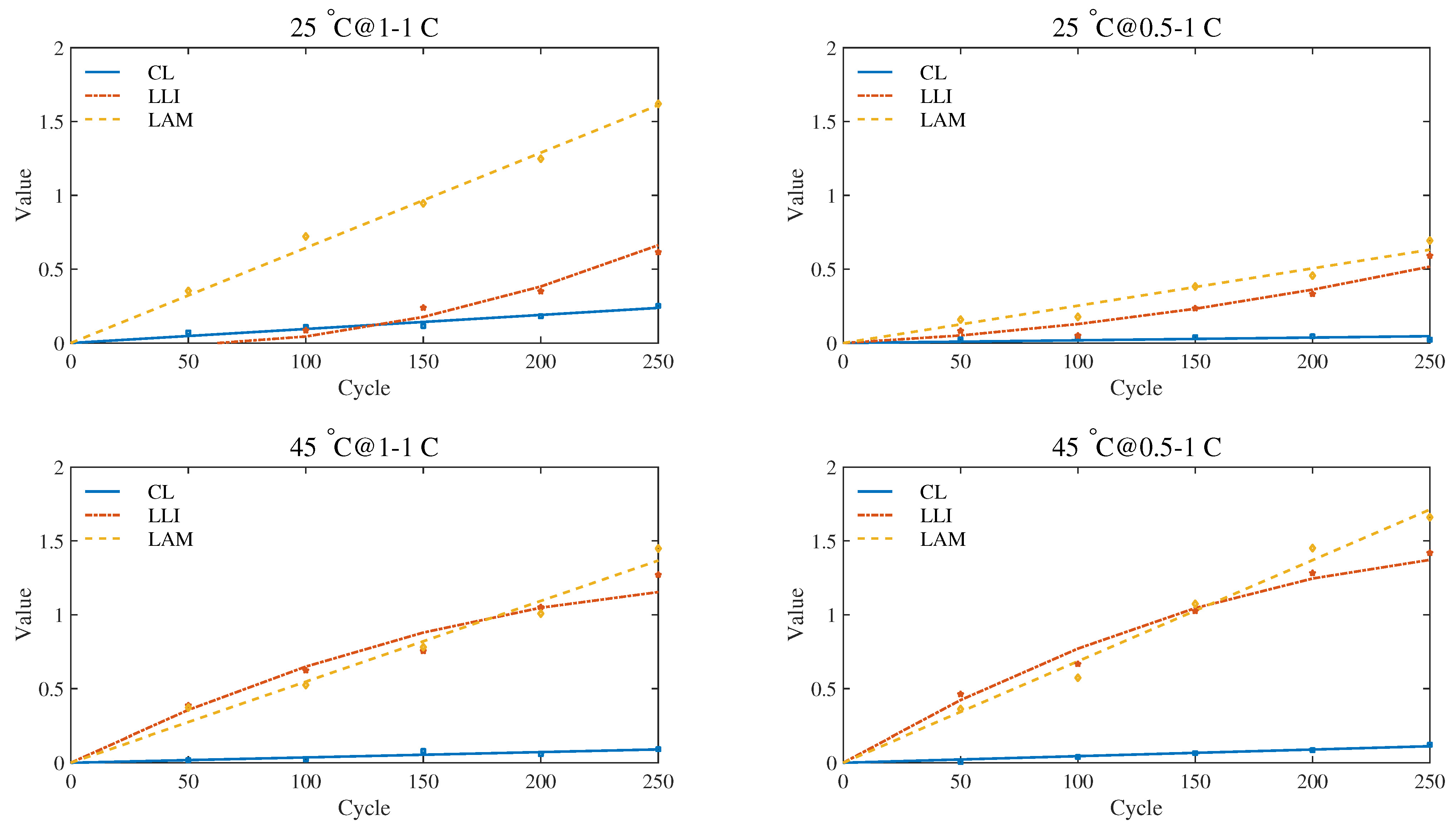
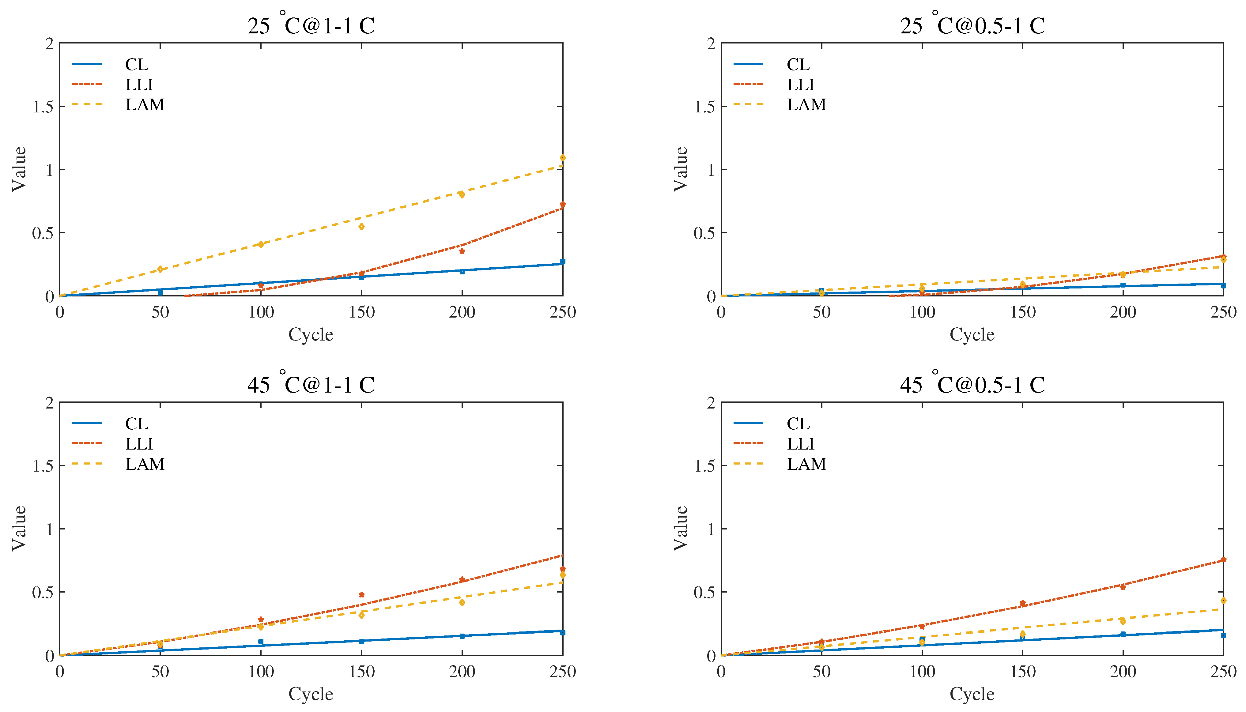
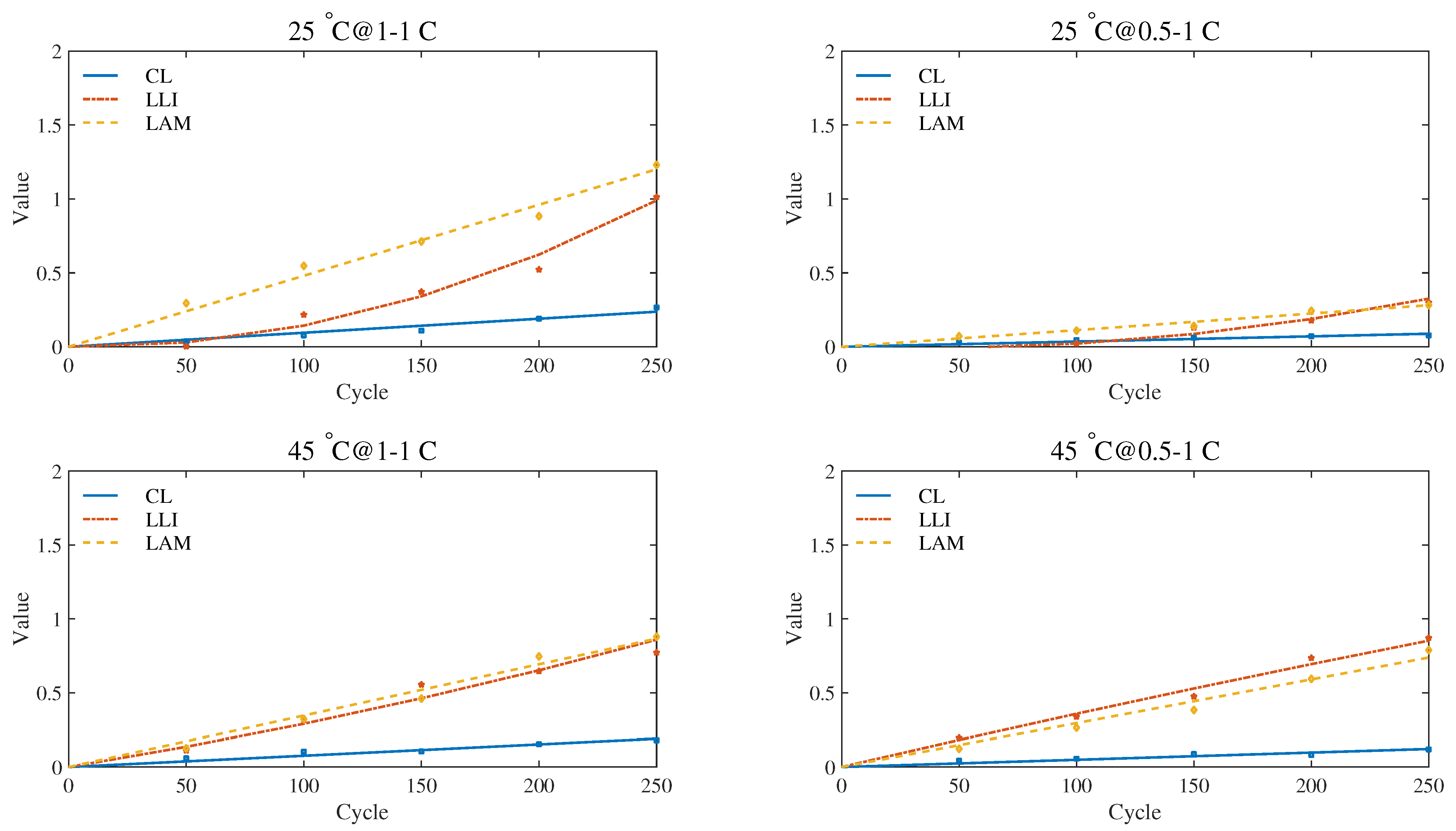
According to the quantification schemes proposed above, the quantitative values of the degradation modes in the first 250 test cycles of the four experimental groups were calculated. When EIS measurement condition is uniformly selected with 500 mA current excitation, the quantitative results recorded at 20%, 50% and 80% SoC are plotted in Figure 10, Figure 11 and Figure 12, respectively.

Observing the quantitative results, we found that, as the aging process progresses, the quantitative values of the three modes show a clear upward trend. Compared with CL, LLI and LAM show more significant growth. This result is consistent with previous studies on aging mechanisms and degradation modes of lithium-ion batteries [20,33,34]. The rapid rise of LLI is mainly due to the continuous growth of SEI films on the surface of the anode materials particles, which is also considered as the main reason for capacity fade in previous studies [35]. However, we found that LAM occupied a similar proportion with LLI, sometimes even higher. This phenomenon has a lot to do with the charge and discharge mode of the cyclic life tests we set, making the batteries always work in a wide SoC range. Frequent deep insertion and extraction of lithium ions will induce greater mechanical stress within the active material particles, which further causing more damage to the electrode material, such as lithiated material loss and particle cracking [19].

Meanwhile, the impact of the operating conditions on the aging mechanism is also well reflected by the quantitative results. Compared with the conditions at 25 ${}^{°}$C, the values of LLI change more significantly at 45 ${}^{°}$C. An important reason for that is the SEI layer on the graphite electrode grows faster at elevated temperatures [36]. The influence of charging current mainly manifests in LAM. As the current decreases, the impact applied to the electrode material during the charging process will be weakened. Accordingly, the increase in the values of LAM is slowed down. CL also shows dependency on charging current and is accelerating at high currents. This result is similar to the ohmic resistance change for various charging rates obtained by Schuster et al. [37]. It indicates that the reaction between the current collector and the electrolyte components is directly or indirectly promoted. Although previous studies [38] have shown that high charging current will also aggravate some side reactions that consume the lithium inventory, such as lithium plating, there is no significant difference in LLI between 0.5 and 1 C. Some scholars [39] have drawn a similar conclusion through ICA. One possible explanation is that a charging current setting of no more than 1 C is not enough to trigger obvious side reactions.

4.2. Effect of SoC and Current Excitation on Quantitative Results

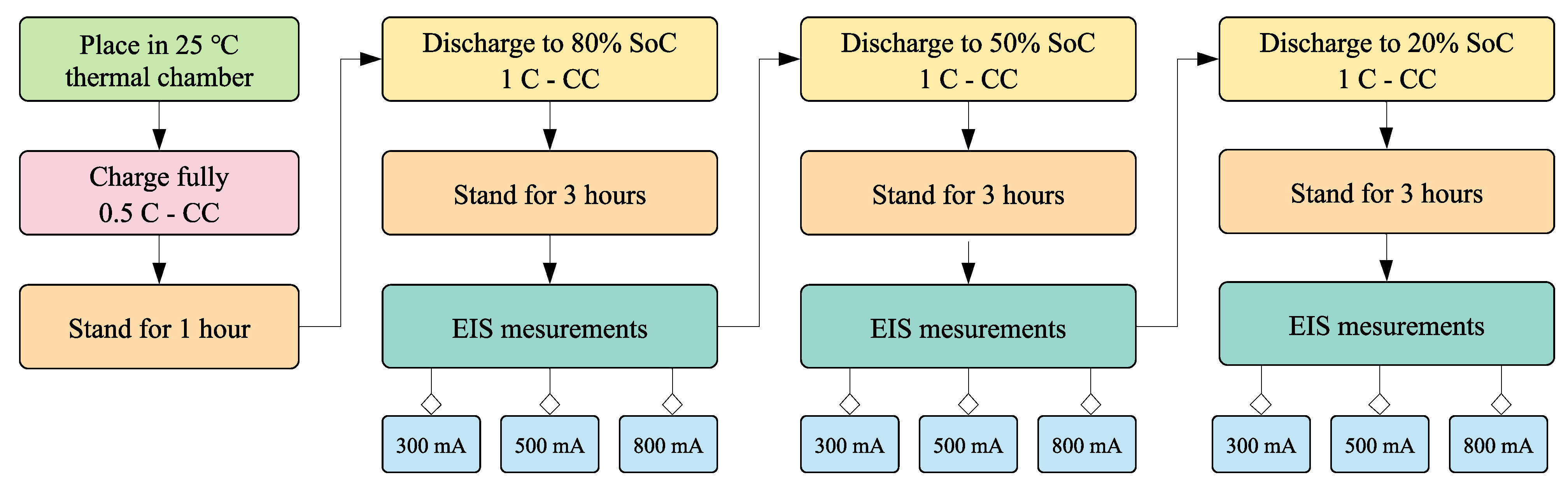
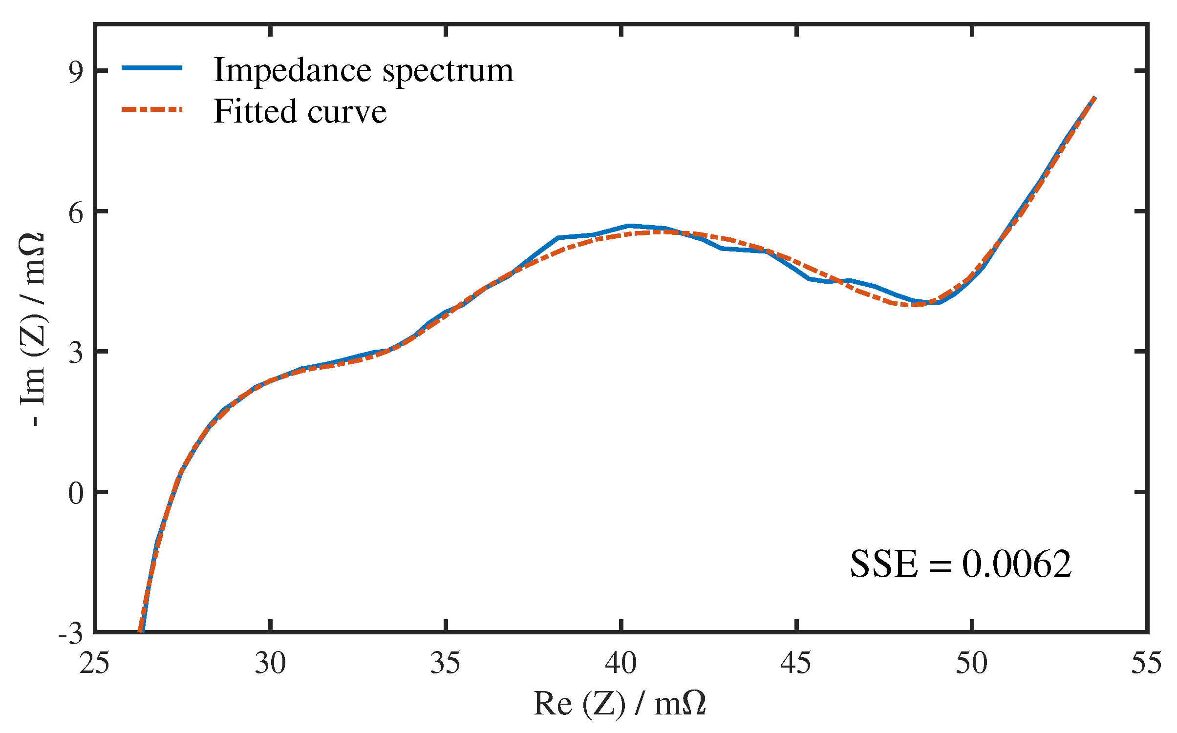
When quantifying the degradation modes, the measuring conditions of EIS were strictly controlled. Different SoC and excitation amplitudes may affect the impedance spectrum curve, which will further affect the resistance values obtained by the equivalent circuit fitting and make the quantitative results change.

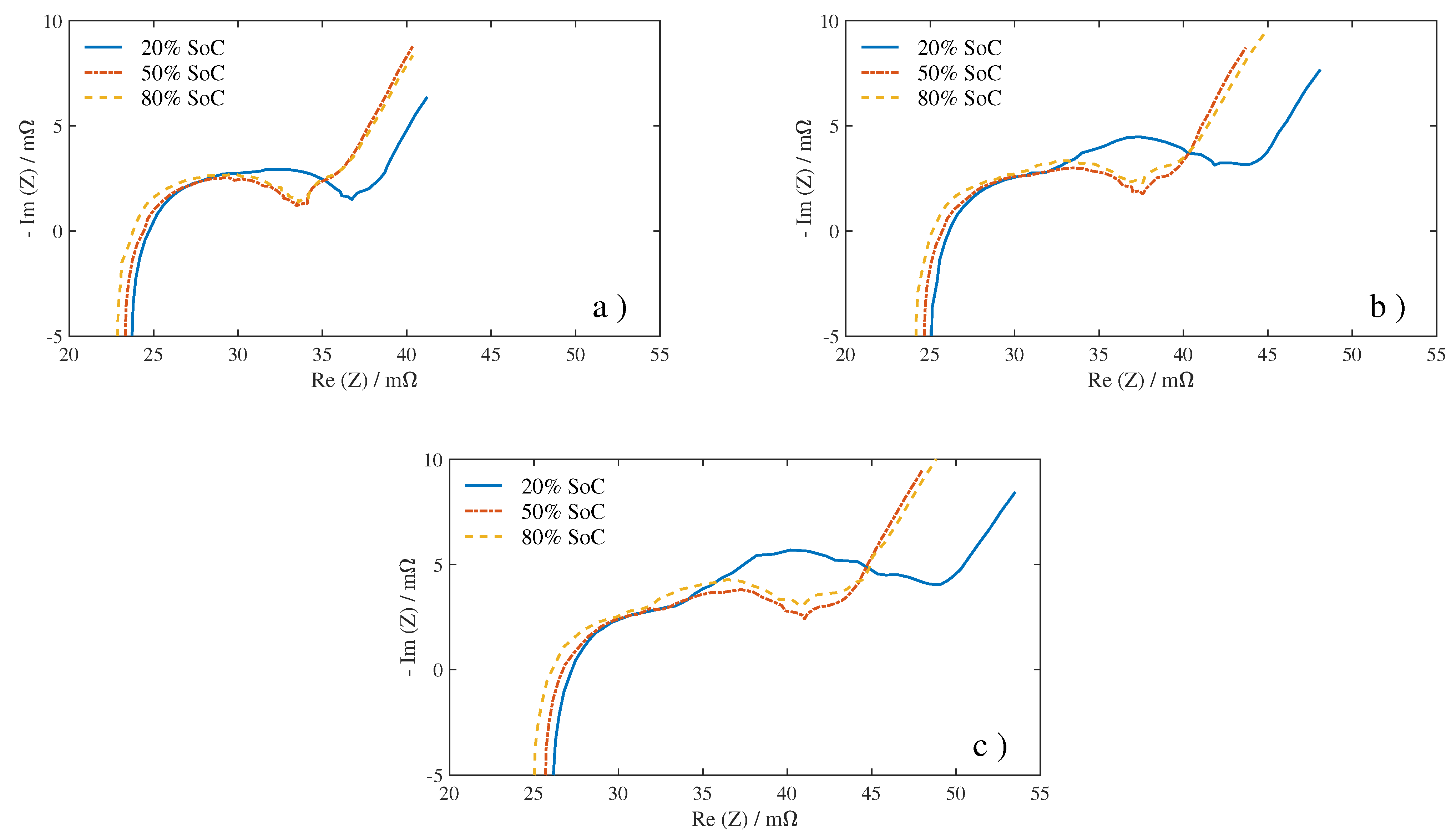
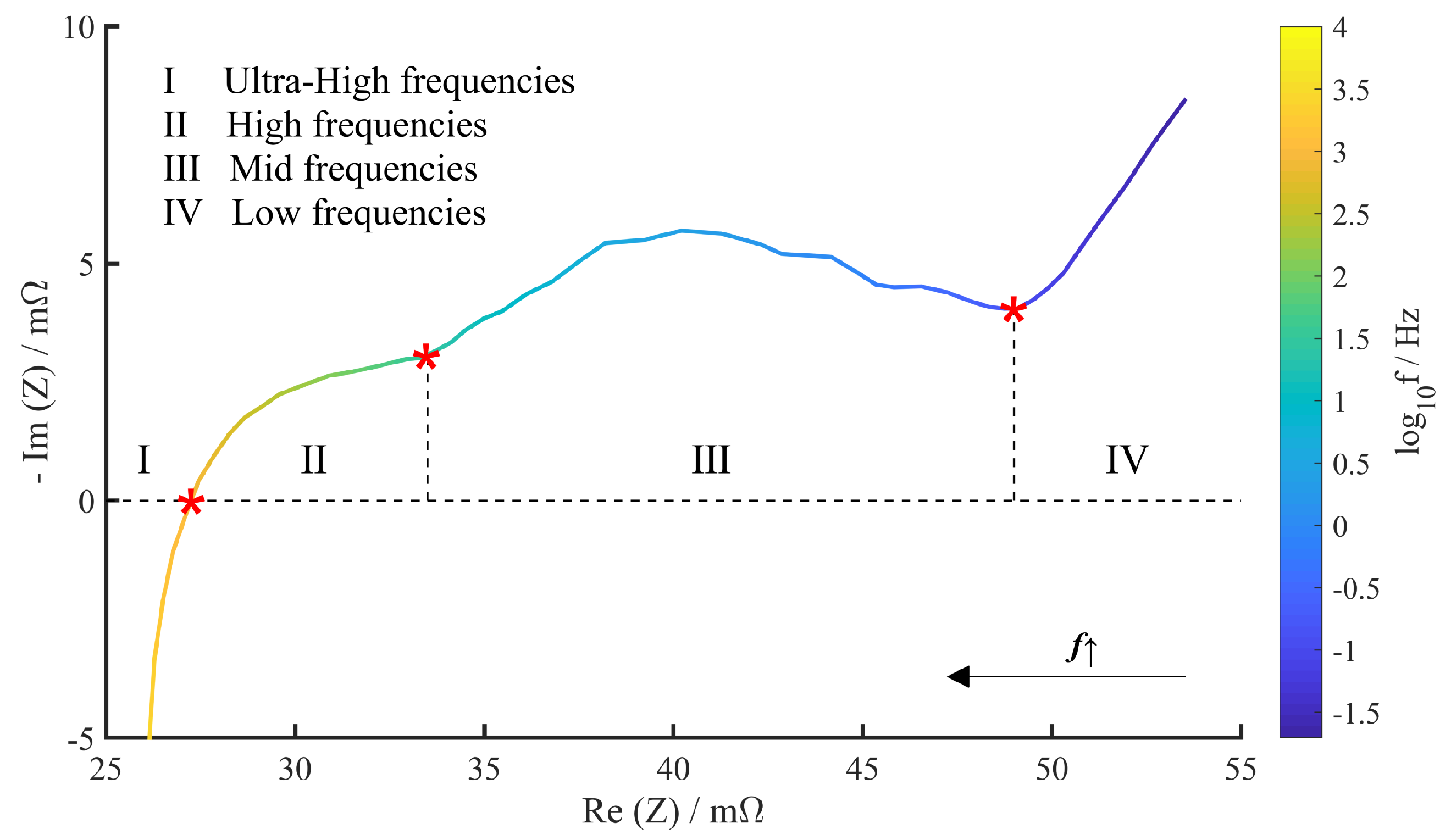
First, we analyzed the influence of SoC and excitation current amplitude on the impedance spectra. The impedance measuring results under 45 ${}^{°}$[email protected]–1 C condition at different SoCs are shown in Figure 13, and the current excitation amplitude is uniformly selected as 500 mA. It can be seen that there is a clear difference between the curves of the three SoCs, especially in mid frequencies and low frequencies. This result is consistent with other studies on EIS. Andre et al. [26] found that the first semi-circle of the spectrum curve shows no significant SoC dependency, but the second semi-circle will spread strongly with declining SoC for SoCs lower than 30%. Since the second semi-circle is closely related to $R_{\mathrm{ct}}$, this phenomenon can also be explained from the perspective of the battery model. Wang et al. [28] conducted a model derivation on the relationship between $R_{\mathrm{ct}}$ and SoC based on the dynamic of the electrode processes, and the results show that $R_{\mathrm{ct}}$ will increase significantly at low SoC.

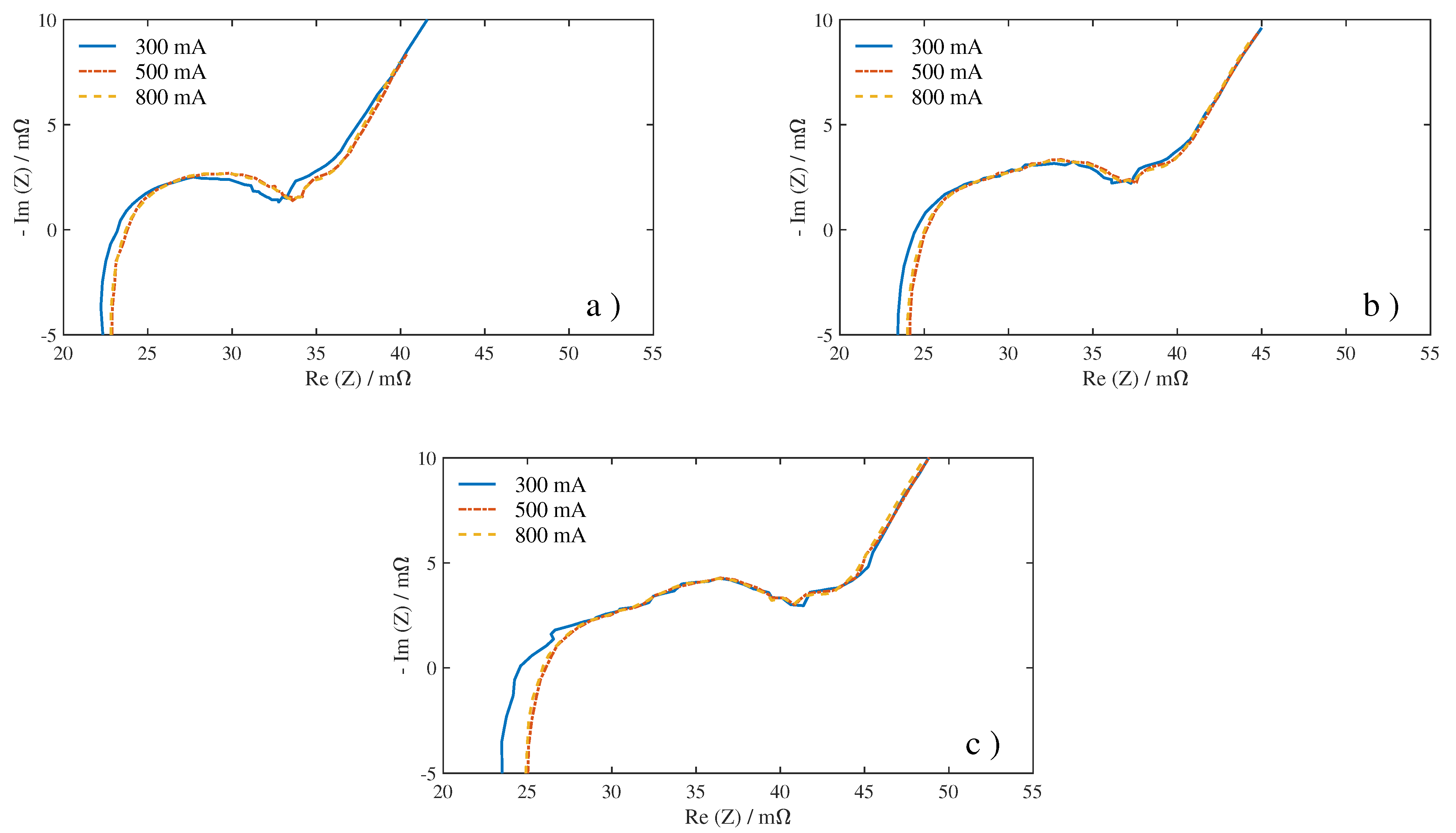
The impedance measuring results under 45 ${}^{°}$[email protected]–1 C condition with different current excitations are illustrated in Figure 14, and the SoC is uniformly selected as 80%. The curves of the three excitation amplitudes roughly overlap together, which means that the excitation has little effect on the change of the impedance spectra. However, compared with 500 and 800 mA, the impedance curve under 300 mA excitation has obvious glitches and bulges. It indicates that the measurement under low current excitation is more sensitive to external noise signals. To avoid the deviation caused by noise, we only consider 500 and 800 mA in the subsequent analysis of the effect of excitation on the quantitative results.

Then, based on the analysis of the impedance spectra, we used two-way analysis of variance (ANOVA) to study and analyze the effect of SoC and current excitation on the quantitative results. ANOVA is a procedure for determining whether variation in the response variable arises within or among different experimental groups [40]. Here, we have two potential influence factors: SoC and excitation current. ANOVA takes the variation due to the factor or interaction and compares it to the variation due to error. If the ratio of the two variations is high, then the effect of the factor or the interaction effect is statistically significant. The statistical significance can be measured using an F-statistic that has an F-distribution [41,42]. A p-value < 0.05 for the F-statistic was considered to be significant. The statistical analysis was accomplished using the function anova2 in Matlab R2018a (The MathWorks, Inc., Natick, MA, USA). For the quantitative results calculated every 50 cycles in the first 400 cycles under 45 ${}^{°}$[email protected]–1 C condition, the statistical results are summarized in

Table 4. The results of two-way analysis of variance under 45 ${}^{°}$[email protected]–1 C condition.

Mode	Source	SS	df	MS	F-Statistic	p-Value
CL	SoC	0.02475	2	0.01237	3.98	0.0253
	Excitation	0.00152	1	0.00152	0.49	0.4887
	Interaction	0.00887	2	0.00443	1.42	0.2506
	Error	0.14939	48	0.00311
	Total	0.18452	53
LLI	SoC	4.8149	2	2.40647	6.79	0.0025
	Excitation	0.0461	1	0.04607	0.13	0.7199
	Interaction	0.1328	2	0.06639	0.19	0.8297
	Error	17.0013	48	0.35419
	Total	21.9931	53
LAM	SoC	12.3921	2	6.19603	10.8	0.0001
	Excitation	0.0837	1	0.08365	0.15	0.7042
	Interaction	0.0764	2	0.03821	0.07	0.9356
	Error	27.5339	48	0.57362
	Total	40.0861	53

. The definitions of the output arguments are listed in

Table 5. The definitions of the output arguments of two-way ANOVA.

Type	Name	Definition
Column	Source	Source of the variability
	SS	Sum of squares due to each source
	df	Degrees of freedom associated with each source
	MS	Mean squares for each source, which is the ratio SS/df
	F-statistic	Ratio of the mean squares
	p-value	Probability that the F-statistic can take a value larger than the computed test-statistic
Row	SoC	Variability due to the differences among the means of SoCs (20%, 50% and 80%)
	Excitation	Variability due to the differences among the means of current excitations (500 and 800 mA)
	Interaction	Variability due to the interaction between SoCs and excitations
	Error	Remaining variability not explained by any systematic source
	Total	Total variability

.

For all degradation modes, the F-statistics corresponding to the SoC factor are far more than one, indicating that the influence of SoC is out of the range of random errors. The p-value for CL is between 0.01 and 0.05, which corresponds to a significant level of more than 95%. The F-statistics and significant level (99%) for LLI and LAM are much higher.

Regarding the excitation factor, the F-statistics of the three modes are all less than one, and the corresponding p-values also far exceed 0.05, which shows that the change of excitation has no significant effect on the quantitative results of each mode.

In addition, for the interaction between SoC and excitation, although the F-statistic value exceeds 1 in CL, the corresponding p-value is higher than 0.05. Therefore, it can be considered that there is no evidence of the interaction effect of the two.

The results of two-way ANOVA show that there is a correlation between SoC and the quantitative results of the degradation modes, especially for LAM and LLI. Next, we further analyzed the specific differences between different SoCs through multiple comparisons using the function multcompare in Matlab R2018a (The MathWorks, Inc., Natick, MA, USA). Multiple comparisons were used to judge whether there is a difference between the estimated group means [43], giving a 95% confidence interval for the true mean difference. The p-value is still used for a hypothesis test that the corresponding mean difference is equal to zero. A p-value < 0.05 was considered a significant difference between the two groups. The results under 45 ${}^{°}$[email protected]–1 C condition and 500 mA excitation are summarized in

Table 6. The results of multiple comparisons between SoCs under 45 ${}^{°}$[email protected]–1 C condition and 500 mA excitation.

Mode	Group	Estimate	95% Confidence Interval		p-Value
			Lower Bound	Upper Bound
CL	20–50%	−0.0516	−0.0966	−0.0066	0.0210
	20–80%	−0.0338	−0.0788	0.0111	0.1743
	50–80%	0.0178	−0.0272	0.0628	0.6076
LLI	20–50%	0.6401	0.1603	1.1199	0.0063
	20–80%	0.6263	0.1465	1.1061	0.0076
	50–80%	−0.0138	−0.4936	0.4660	0.9973
LAM	20–50%	1.1398	0.5292	1.7504	0.0001
	20–80%	0.8114	0.2008	1.4220	0.0065
	50–80%	−0.3284	−0.9390	0.2822	0.4017

.

Observing the data, we found that the difference mainly existed between low SoC (20%) and medium-high SoC (50%, 80%). There is a very significant statistical difference in LLI and LAM values between 20% SoC and the other two SoCs, featured with the confidence intervals excluding zero and the p-values less than 0.01. In contrast, the difference between 50% SoC and 80% SoC is not significant (p-value ≫ 0.05). Combined with the quantitative results of the same condition at different SoCs shown in Figure 10, Figure 11 and Figure 12, this difference is mainly manifested in the larger LAM and LLI values at 20% SoC, which is in agreement with the study of Pastor-Fernández et al. 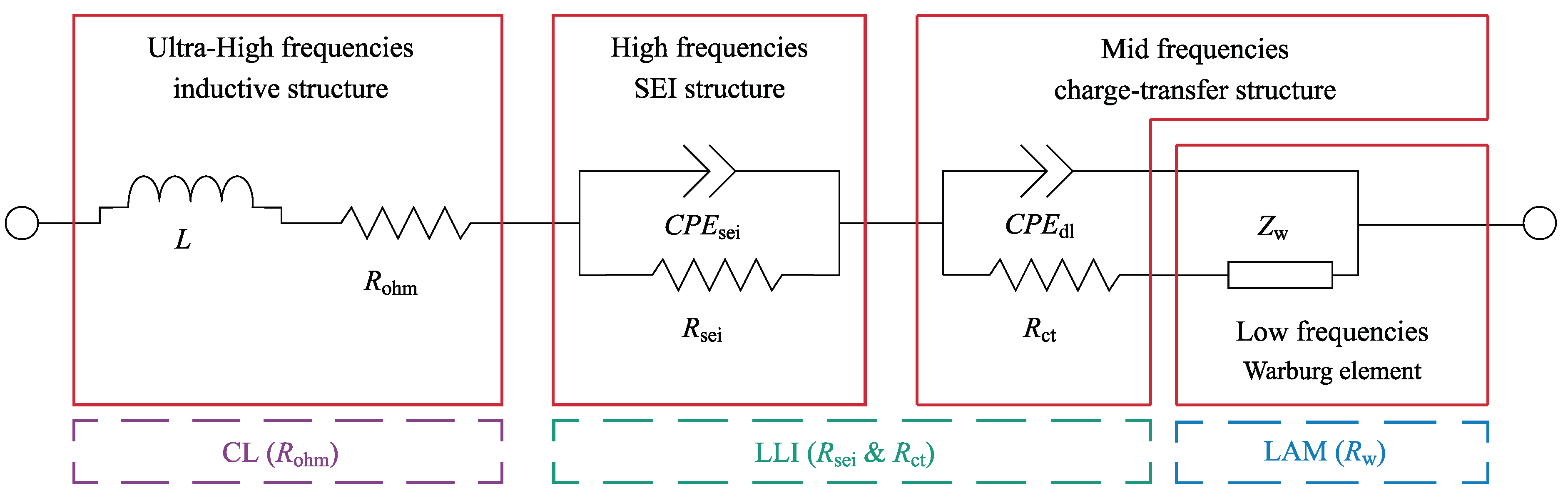[10] under 25 ${}^{°}$[email protected]–1 C condition. This phenomenon is related to the characteristics of the impedance spectrum, as described above. Due to the expansion of the second semi-circle, the fitted values of $R_{\mathrm{ct}}$ ($R_{\mathrm{c}}$) and $R_{\mathrm{w}}$ are significantly different at 20% SoC, and then bring the difference in the quantified values of LLI and LAM. For CL, the difference is principally between 20% SoC and 50% SoC (0.01 < p-value < 0.05), but, overall, the significant level is much lower than the other two modes. Combining the quantification method, this result is determined by the characteristics of $R_{\mathrm{ohm}}$, which shows no significant dependency on SoC [44].

5. Conclusions

Based on the EIS method, this paper proposes a new quantification method that uses two equivalent circuit models to fit the impedance curves jointly and extends the quantitative study of degradation modes to various conditions. Combining the two external factors of SoC and excitation current, the quantified values of degradation modes under different conditions are explored. The main conclusions are summarized as follows.

(1)

The shapes of the impedance spectra may show two different change trends during the aging process. For conditions where there are not two distinguishable semi-circles in the medium-high frequency region, the second-order model is changed to the first-order model according to the characteristics of impedance changes. Besides good impedance curve fitting results, a proper model also provides resistance values consistent with aging mechanisms for subsequent quantitative analysis. The quantification methods based on the two models not only ensure the corresponding relationship between degradation modes and resistance characteristics but also provide accurate and comparable results for quantitative analysis under different conditions.

(2)

It was verified by experiments that, under different conditions, LLI and LAM always dominate the aging process. For LLI, ambient temperature is the deciding factor, and a higher temperature means a larger lithium-ion loss rate. By contrast, LAM and CL are more closely related to the charging current and can be restrained by reducing the current. Even though many studies have confirmed that large currents promote side reactions such as lithium plating, no significant correlation between charging current and LLI is observed under conditions designed in this article.

(3)

The selection of SoC during EIS measurement has an important influence on the quantitative result. The effects of SoC on LAM and LLI are mainly manifested between low SoC (20%) and medium-high SoC (50%, 80%). At low SoCs, larger quantified values can be obtained. However, CL is relatively consistent at different SoCs on account of the characteristics of ohmic resistance. The effect of excitation current on the results is not significant. However, from the perspective of the reliability of quantified values, it is necessary to avoid selecting an excitation current that is too low to prevent excessive noise during EIS measurement.