Study on Outlet Temperature Control of External Receiver for Solar Power Tower

Abstract

Due to the change of direct normal irradiance (DNI) and the change of output power load, the receiver of the solar tower is in an unstable state in the actual operation. In this paper, a 100 MW external cylindric receiver is designed and modelled. The dynamic and comprehensive model is established for the receiver, including the thermal and mechanical equations. The temperature control strategy is applied to the receiver model. The validity of the control strategy is verified by disturbance experiments, including DNI, the inlet temperature of the heat transfer fluid (HTF), and the weather data on a cloudy day. The response characteristics of the receiver are demonstrated. Its thermal lag characteristics and restraining effect on the fluctuating environment are revealed. The dangerous occasion of the receiver during operation are detected, including the overheat of the local panel, and the dissociation point of the molten salt. Both the robustness and the deficiency of the control strategy of the receiver are pointed out. The research results will contribute to the control strategy formulation of the SPT (solar power tower) station.

1. Introduction

Growth in carbon emissions slowed down in the previous year, as primary energy consumption decelerated and renewables displaced coal from the energy mix. Renewable energy posted a record increase in consumption in energy terms. As a promising renewable utilization technology, integration of concentrated solar energy and heat storage provide a stable power source for the power grid. The intermittent and volatility of solar energy can be harnessed by thermal energy storage, so as can the CSP (concentrated solar power) plant use it for the peak load regulation of the electric power system. Thermal energy storage (TES) is essential to adjust the mismatch between the irregular supply of renewable energy and user demand. Furthermore, the cost reduction of TES (USD 16/kWh-thermal) can reduce the investment of the CSP plant significantly [1,2].

Among all the CSP technologies, tower power is prominent for its merits, such as high efficiency and low investment cost. These benefits contribute to the development of the large-scale (50–1000 MW) CSP power plant [3]. In a multi-energy complementary system, the STP plant equipped with thermal storage can levelize the fluctuation of the power output [4]. The challenges to the STP come from two aspects—the volatility of the solar and wind and the unpredictability of the power load in demand. The heat transport characteristics of such an STP which may work under variable conditions frequently are prominent.

The heat transport characteristics of STP is mainly embodied in the three subsystems—the receiver system, the steam generation system, and the steam turbine power cycle system. The receiver is very sensitive to the constantly changing direct normal irradiation (DNI) as the heat source of the plant.

The previous studies mainly focus on analyzing and improving the thermal performance of the receiver. Some researchers investigate the transient characteristics and operation analysis of the receiver.

For the first category, Sánchez compared the allowable flux density of different materials of the receiver and analyzed the thermal stress [5]. For the receiver efficiency improvement, the fin-like receiver is proposed, and the designed parameters are optimized. Compared with the cylindrical receiver, efficiency is improved by 3.8% [6]. In the case of uneven heat flux, nanofluids were mixed with molten salt to enhance heat transfer and reduce the temperature of the receiver [7]. A single tube is chosen for the object to present the fatigue fracture and thermal stress in the condition of uneven heat flow. The results show that the molten salt thermal distribution along the circumferential and axial directions is obviously non-uniform, and the wall temperature distribution is much related to the inlet velocity of molten salt [8]. For the heat transfer reinforcement, a novel spiral tube is used as the absorber tube in the receiver, and the experimental results display that the Nusselt numbers are in the range of 400–1200, which is about three times the normal one [9].

For the second category, Yu studied the dynamic characteristics of molten salt receivers with step perturbation, and the impact of different parameters on the receiver is studied [10]. Zhang developed a test method for the time constants of the receiver, which is a key indicator of the dynamic characteristics of the receiver [11]. Both the dynamic simulation and the experiment are carried out for the molten salt receiver, and 11 sets of transient working conditions are studied by Zhang [12]. The receiver system, comprised of a receiver and cold and hot surge tanks, is modelled to test the function of surge tanks under the condition of pump failure and downcomer blocker [13]. The thermal stress and tube deflection in the receiver under uneven solar flux is analyzed by transient modelling and experiment [14]. Both the direct-filling and S-type flow mode are tested by Li to demonstrate the flow distribution and surface temperatures, and the results show that the S-type mode has better performance to prevent solidification under cloudy conditions [15].

The previous study focusses on the thermal performance analysis, transient characteristics, and the operational performance of the molten salt receiver. But the control strategy of the molten salt receiver against the frequently changing environment is rarely concerned.

In this study, the comprehensive model of the external cylindric solar receiver utilized in the SPT plant is developed. In the model, the heat absorption of the receiver, the convection loss, and radiation loss under the changing environment are calculated. The coupled solution of velocity and pressure is adopted. The control strategy is applied to the receiver for temperature regulation. The disturbance experiments, including DNI (direct normal irradiation), cloud passage, the molten salt inlet temperature, and the weather data on a cloudy day, are carried out to test the validity of the receiver control strategy. The results show that the control strategy has good robustness. Moreover, the emergency conditions are detected, including the overheat of the absorber tubes and the dissociation of the molten salt. Based on the results, the aiming strategies and control methods can be more accurate for the receiver.

2. Model Description

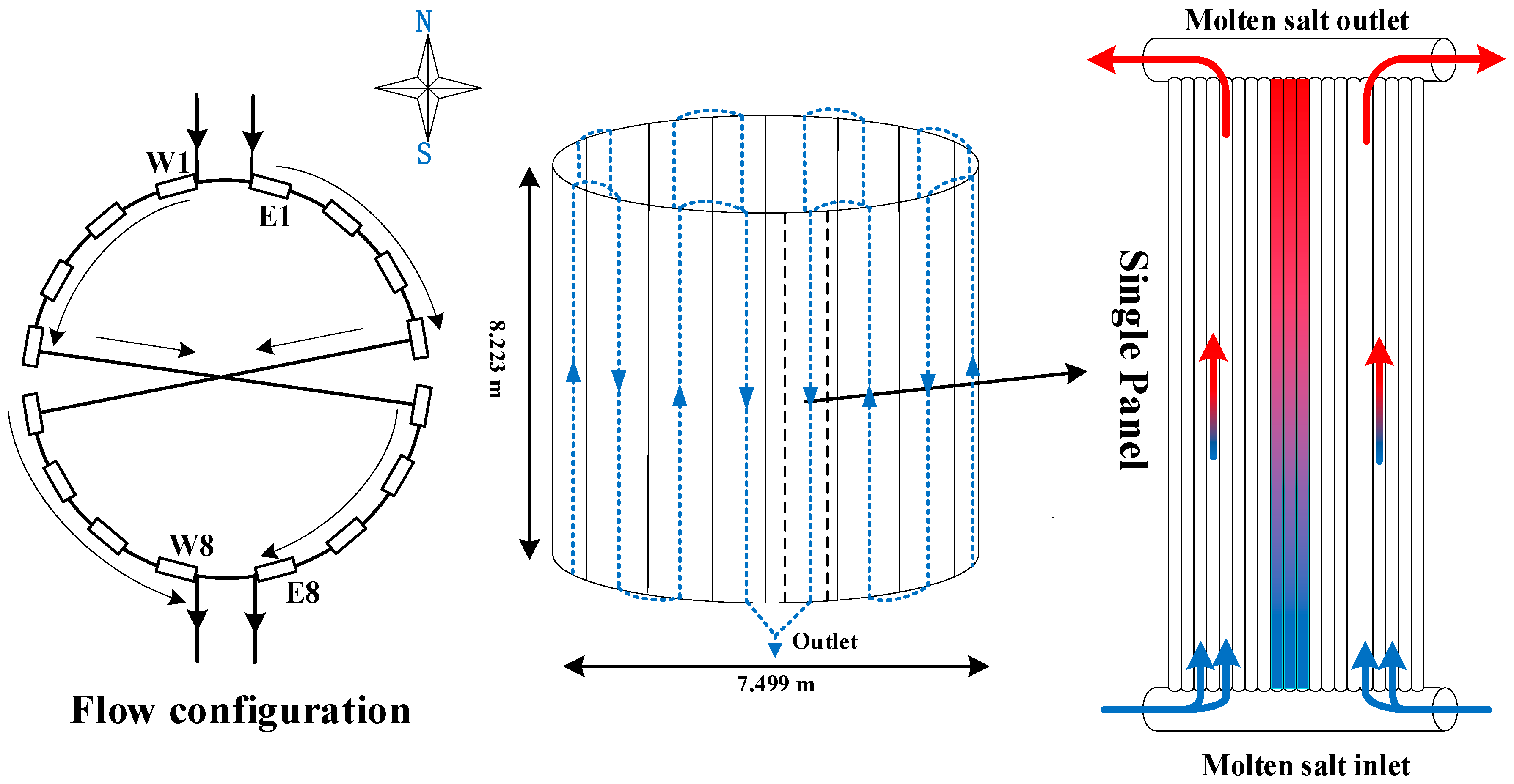
2.1. Designed Receiver Model

Based on the criterion of paper [16], a 100 MW external receiver which uses molten salt as the HTF is designed. The structure of the designed receiver is displayed (Figure 1). The molten salt enters the receiver from the north, and proceeds in sequential panels until the middle of the receiver, then there is a crossover between the east and west.

The dimension parameters are displayed in

Table 1. Receiver parameters.

Key Parameters	Designed Value
Heat load, MW	100
Area, m2	192.49
Aspect ratio	1.11
Tube external diameter, m	0.0209
Tube internal diameter, m	0.0185
Unit width, m	1.463
Tube number/unit	70
Receiver diameter, m	7.499
Receiver height, m	8.223
Panel number	16
Heliostat field efficiency, %	51.026
Mirror aperture, m2	20
Rated DNI, W/m2	800
Number of heliostats	15,310

. The parameters of the receiver are optimized, especially the inner diameter and wall thickness. The material of the receiver is AISI316 stainless steel. The heliostat field efficiency remains constant. The simplification method in the study of Li and Zhang et al. [16,17] is adopted here.

2.2. Material Properties

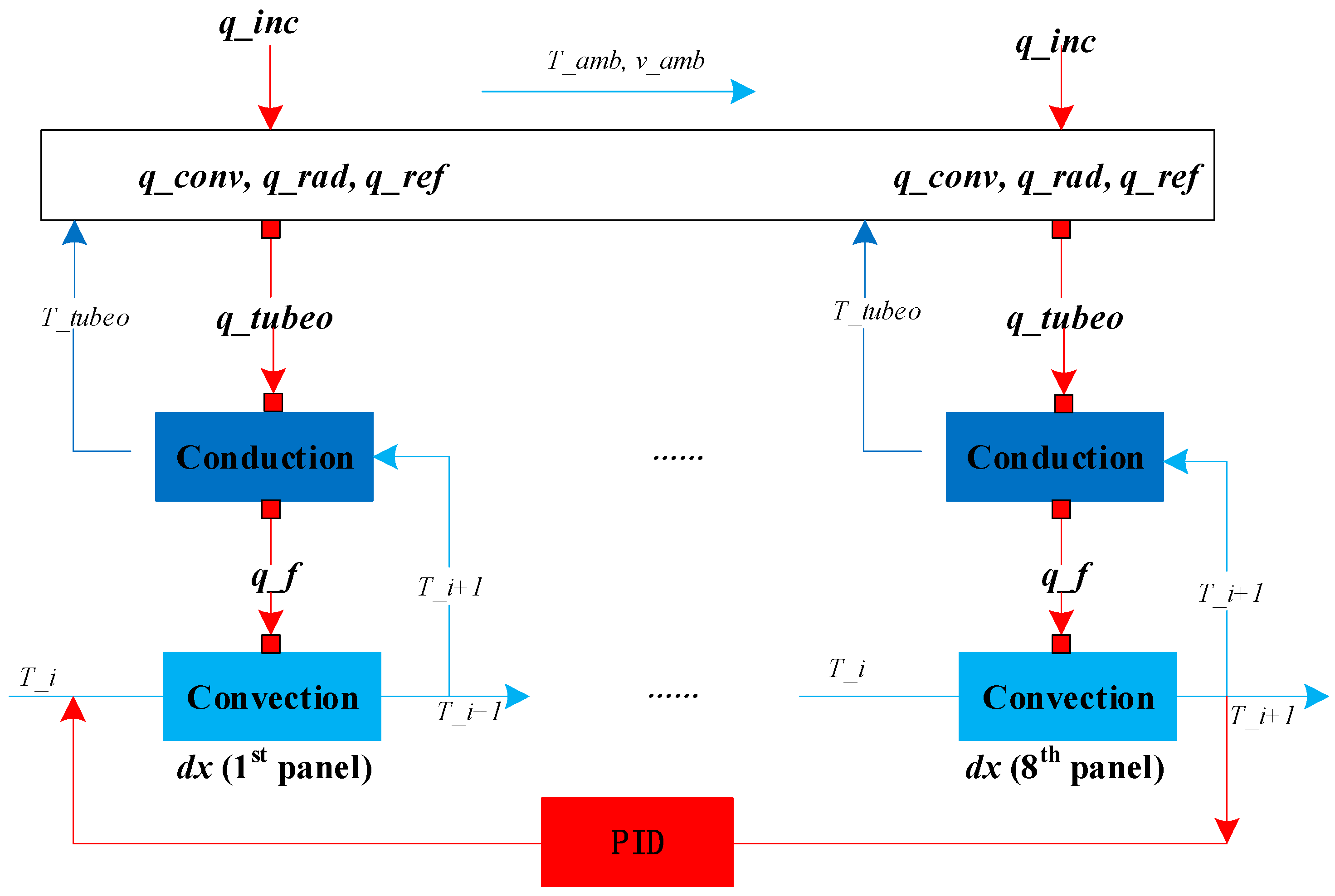
The HTF used in the receiver is the mixture of 60% NaNO₃ and 40% KNO₃. The stability and low cost are the two main reasons for material selection. The physical characteristics of solar salt are shown in our previous paper [17]. The equations of the stainless steel properties are listed in

Table 2. Relations of tube material properties with temperature.

Property	Function
Coefficient of thermal expansion, °C	${\alpha }_{steel}=15.8+0.6\times {10}^{-2}\left(T-24.85\right)$
Specific heat, kJ/kg, °C	$C_{p\_steel}=472+13.6\times {10}^{-2}\left(T-293.15\right)-2.82\times {10}^6/{\left(T-293.15\right)}^2$
Density, kg/m3	${\rho }_{steel}=7950-0.501\left(T-25\right)$

.

2.3. Dynamic Model

The receiver is operated around a high concentrated solar radiant flux (around 600–1200 times of horizontal surface DNI). The design and the operation of the receiver face the great challenge of high flux concentration. Many researchers make efforts on how to allocate the heat flux evenly to avoid thermal failure. The working condition is complicated with ambient conditions. The flux concentration can be affected by many factors such as sky clarity and the heliostat field layout. The change of wind speed, atmospheric temperature, and pressure as weather changes can make the working condition harder for the receiver. For the molten salt in the receiver has to endure high working temperature, corrosion fatigue may appear. During varying output power load, if not designed or operated properly, great thermal stress and fatigue could occur.

To lay a foundation for the heat transport and operation analysis of the receiver, a detailed and comprehensive model is developed. The result of the energy balance for each panel is represented by a single vertical tube and can be scaled by the number of tubes in that panel. Each absorbing tube is discretized into N control volumes along the molten salt flow direction. The energy balance for an element in a single tube is illustrated in Figure 2. The solution to the mathematic model is the Runge–Kutta algorithm. The time step is 0.1 s. Assumptions and simplifications of the model are stated bellow.

(1)

Tube-to-tube conduction and radiation exchange is ignored;

(2)

Axial conduction between the adjacent control volumes is neglected because the convection between the inner wall of the tube and the molten salt dominates the heat transfer in the tube.

2.3.1. Energy Collection

Energy flux density and heat losses calculation of the receiver,

$$q_{\mathrm{tube},\mathrm{o}}=q_{\mathrm{inc}}-\left(q_{\mathrm{ref}}+q_{\mathrm{rad}}+q_{\mathrm{conv}}\right)$$

(1)

$$q_{\mathrm{inc}}=P_{\mathrm{field}}·D_{\mathrm{tube}}·n_{\mathrm{tube}}·dx$$

(2)

$$q_{\mathrm{ref}}=\left(1-\alpha \right)D_{\mathrm{tube}}{P}_{\mathrm{field}}{n}_{\mathrm{tube}}dx$$

(3)

$$q_{\mathrm{rad}}=\sigma \epsilon \pi \frac{D_{\mathrm{tube}}}{2}{F}^{*}{}_{\mathrm{tube}}{D}_{\mathrm{tube}}{n}_{\mathrm{tube}}\left(T_{\mathrm{tube},\mathrm{o}}^4-T_{\mathrm{amb}}^4\right)dx$$

(4)

where ε, σ, α, and $F_{tube}^{*}$ represent the emissivity of Pyromark, Boltzmann constant, hemispherical absorptivity of absorbing tubes, and angular coefficient and their value, respectively [18].

The convection loss of panel unit,

$$q_{\mathrm{conv}}=h_{\mathrm{m}}^{*}{D}_{\mathrm{tube}}{n}_{\mathrm{tube}}\left(T_{\mathrm{tube},\mathrm{o}}-T_{\mathrm{amb}}\right)dx$$

(5)

$$h_{\mathrm{m}}^{*}={\left({{\displaystyle {{\displaystyle h}}_{\mathrm{fo}}^{*}}}^a+{{\displaystyle {{\displaystyle h}}_{\mathrm{nat}}^{*}}}^a\right)}^{1/a}$$

(6)

where $h_{\mathrm{fo}}^{*}$ and $h_{\mathrm{nat}}^{*}$ are the convection coefficient of the receiver surface under different working conditions. When only the forced convection is considered, $h_{\mathrm{fo}}^{*}$ is acquired. $h_{\mathrm{nat}}^{*}$ is acquired when only the natural convection is considered. a is the comprehensive correlation factor of $h_{\mathrm{fo}}^{*}$ and $h_{\mathrm{nat}}^{*}$ [19].

The Nusselt number can be calculated by the following equations,

$$N{u}_{\mathrm{nat}}=0.098G{r}_{\mathrm{rec}}^{1/3}{\left(\frac{T_{\mathrm{tube},\mathrm{o}}}{T_{\mathrm{amb}}}\right)}^{-0.14}$$

(7)

$$G{r}_{\mathrm{rec}}=g·\beta ·\left(T_{\mathrm{tube},\mathrm{o}}-T_{\mathrm{amb}}\right)·\frac{H_{\mathrm{rec}}^3}{v_{\mathrm{amb}}^2}$$

(8)

The value of D_tube/D_rec and the calculation of heat transfer coefficient of forced convection are selected in [20].

2.3.2. Tube Wall Conduction

The solar irradiation is concentrated on the surface of absorber tubes by heliostats. By heat conduction, heat is transmitted through the metal to the inner wall. The conduction and convection are coupled by the following equation The axial conduction is ignored. In the equations of unsteady heat conduction, the thermal inertia of the metal is considered.

$$\{\begin{array}{l}{R}_{\mathrm{tube}}=\frac{ln\left(\frac{r_{\mathrm{tube},\mathrm{o}}}{r_{\mathrm{tube},\mathrm{in}}}\right)}{2\pi k_{\mathrm{s}}dx}\\ q_{\mathrm{tube},\mathrm{in}}=\frac{T_{\mathrm{tube},\mathrm{o}}-T_{\mathrm{tube},\mathrm{in}}}{R}\\ m_{\mathrm{tube}}{c}_{\mathrm{tube}}\frac{d{T}_{\mathrm{tube}}}{dt}=q_{\mathrm{tube},\mathrm{o}}-q_{\mathrm{tube},\mathrm{in}}\\ \end{array}$$

(9)

2.3.3. Internal Convection

By heat convection, heat is transmitted to the HTF from the inner wall. Principle of mass conservation, energy conservation, and momentum conservation are described by the following equations. i represents the control volume (CV), and i + 1 is the next CV.

Mass conservation:

$$\{\begin{array}{l}\frac{d{M}_{\mathrm{i}}}{dt}={\dot{m}}_{\mathrm{i}}-{\dot{m}}_{\mathrm{i}+1}\\ M_{\mathrm{i}}={\rho }_{\mathrm{i}}{V}_{\mathrm{i}}\\ V_{\mathrm{i}}=\pi r_{\mathrm{s},\mathrm{inner}}^2\cdot dx\\ {\rho }_{\mathrm{i}}=f\left(T_{\mathrm{i}}\right)\end{array}$$

(10)

Energy conservation:

$$\{\begin{array}{l}\frac{d\left(M_{\mathrm{i}}{u}_{\mathrm{i}}\right)}{dt}=q_{\mathrm{salt},\mathrm{i}}-\left({\dot{m}}_{\mathrm{i}+1}{h}_{\mathrm{i}+1}-{\dot{m}}_{\mathrm{i}}{h}_{\mathrm{i}}\right)\\ q_{\mathrm{salt},\mathrm{i}}=h_{\mathrm{salt},\mathrm{i}}^{*}{A}_{\mathrm{salt},\mathrm{i}}\left(T_{\mathrm{tube},\mathrm{in},\mathrm{i}}-T_{\mathrm{i}}\right)\\ u_{\mathrm{i}}=h_{\mathrm{i}}-P_{\mathrm{i}}/{\rho }_{\mathrm{i}}\end{array}$$

(11)

The heat absorbed from the sun by the tube is equal to that transmitted to the HTF.

$$q_{\mathrm{salt},\mathrm{i}}=q_{\mathrm{tube},\mathrm{in}}$$

(12)

The calculation method of Nusselt number for convection in the tube can be found in [17].

Momentum conservation:

The relation between the velocity and pressure is included in the model,

$$\{\begin{array}{l}{A}_{\mathrm{tube},\mathrm{in}}\left({\rho }_{\mathrm{i}-1}\cdot v_{\mathrm{i}-1}^2-{\rho }_{\mathrm{i}}\cdot v_{\mathrm{i}}^2\right)=F_{\mathrm{p},\mathrm{i}}+F_{\mathrm{g},\mathrm{i}}+F_{\mathrm{friction},\mathrm{i}}\\ F_{\mathrm{p},\mathrm{i}}=A_{\mathrm{tube},\mathrm{in}}\left(P_{\mathrm{i}}-P_{\mathrm{i}-1}\right)\\ F_{\mathrm{friction},\mathrm{i}}=\frac{1}{2}\left({\rho }_{\mathrm{i}-1}+{\rho }_{\mathrm{i}}\right)\frac{\Delta P_{\mathrm{salt},\mathrm{i}}}{{\rho }_i}\cdot A_{\mathrm{tube},\mathrm{in}}\\ \frac{\Delta P_{\mathrm{salt},\mathrm{i}}}{{\rho }_i}=f_D\frac{dx}{2r_{\mathrm{tube},\mathrm{in}}}\cdot \frac{v_{\mathrm{i}}^2}{2g}\end{array}$$

(13)

In the ideal case, F_g,i can be ignored. The gravity effect is offset for the ascension pipes, and downcomers can complement each other. The friction is considered during the flow process. Darcy formula is adopted to calculate the pressure drop [21].

2.3.4. Thermal Stress

Among all the thermal stresses of the tube, the tangential one has the greatest influence. For a certain type of tube, tangential thermal stress is a function of the temperature gradient,

$${\sigma }_{\mathrm{axial}}=\frac{\Delta T_{\mathrm{w}}\alpha E}{2\left(1-\nu \right)ln\left(\frac{r_{\mathrm{o}}}{r_{\mathrm{i}}}\right)}\left(1-\frac{2r_{\mathrm{i}}{}^2}{r_{\mathrm{o}}^2-r_{\mathrm{i}}^2}ln\left(\frac{r_{\mathrm{o}}}{r_{\mathrm{i}}}\right)\right)$$

(14)

The value of E and v is selected in [17].

2.4. Control Strategy

In the receiver system, the object of the control strategy is to regulate the temperature at the calibration value to escape generating large thermal stresses in the heat exchange components. Therefore, the mass flux of the molten salt should be adjusted to adapt to the real-time DNI. The mass flux is a way to adjust the temperature of the outlet of the receiver.

By the flow rate regulation of the control strategy, the salt outlet temperature is controlled. The salt outlet temperature is also the feedback signal of the controller. In view of the feedback signal and the mass flux of the salt, the control system sends commands to the molten salt pump.

The proportion integration differentiation control algorithm is used in the control system. The control variable of the control system is the flow rate of molten salt. The outlet temperature of the molten salt is the main signal, and the mass flux of the salt is the feedforward signal. The typical unit negative feedback control method is used to regulate the two parameters.

$$v(t)=K_g\left(e(t)+\frac{1}{t_i}{\displaystyle \underset{0}{\overset{t}{\int }}e(\tau )\mathrm{d}\tau +t_d\frac{\mathrm{d}e(t)}{dt}}\right)=P_c+I+D_c$$

(15)

where e is tracking error.

The molten salt pump takes action according to the feedback and the feedforward signals from the control system. The control strategy aims to levelize the salt outlet temperature at the rated value.

2.5. Simulation Method

One of the targets of this paper is to reveal the temperature distribution along the molten salt flow direction. So the one-dimensional fluid flow pattern is chosen. The schematic of the modelling procedure is described in Figure 2. N finite control volumes are acquired by discretizing each tube of the panel. The inlet and outlet temperature of flow fluid control volume are T_i and T_i+1, respectively. The relation between the mass flux and the pressure of adjacent control volumes is specified by the momentum balance equation.

The calculation procedure is displayed in Figure 3. Solar energy is collected by the receiver. Incident energy is cut down by the scattering and absorbing of the air. Given the temperature of the tube, all and ambient parameters, q_rad and q_conv are calculated. By convection, the rest of the heat is transmitted to the HTF. Then T_{_i+1} is sent back to the wall conduction module. Then the value of q_f is renewed. The heat conduction of molten salt is displayed in Figure 2. Heat reduction in the axial direction is ignored. For the equation solution, the Runge–Kutta algorithm is used. MATLAB language is used as the programming language. The single absorbing tube is discretized into 164 control volumes. The time step of the simulation is 0.1 s.

2.6. Model Validation

The receiver design criteria of paper [16] are applied in this paper. Based on the conservation of energy, mass, and momentum, the receiver is modelled mathematically. Then the one-dimensional transient model is calculated and validated by contrast to the designed value. The calibration value of the HTF temperature for a molten salt external receiver is 290 °C (inlet) and 565 °C (outlet) in [22]. The calculation value of the molten salt outlet temperature is 569.74 °C, thus lower than 0.84% relative error is achieved. The reliability of the present model is validated.

To further reinforce the validation, uneven heat flux is adopted to investigate the temperature distribution along the flow direction, and the trends of molten salt temperature are compared with [23]. Although the two receivers in the different article have difference thermal duty (114.7 to 100 MW) and various working conditions, their temperature trends (T__tubeo and T_{_salt}) under uneven heat flux (Gaussian) are coincident (in Figure 4a,b). The molten salt outlet temperature is around the rated value, higher than that in this paper which is below 500 °C. In addition, the design heat flux on the receiver in the reference paper is higher compared with that in this paper (875.29 to 519.5 kW/m² of the design heat flux). The working condition in the reference paper is more ideal. For the security consideration of actual operation, the lower allowable heat flux density is selected for the receiver design. Additionally, it is an optimized value in consideration of the geometric parameters and the thermal efficiency [16]. The temperature difference between the tube and the molten salt is higher than that in the reference paper, since a different material is used. However, the temperature distribution along the flow direction of the two models have the same trend, including the temperature of the tube wall and the molten salt.

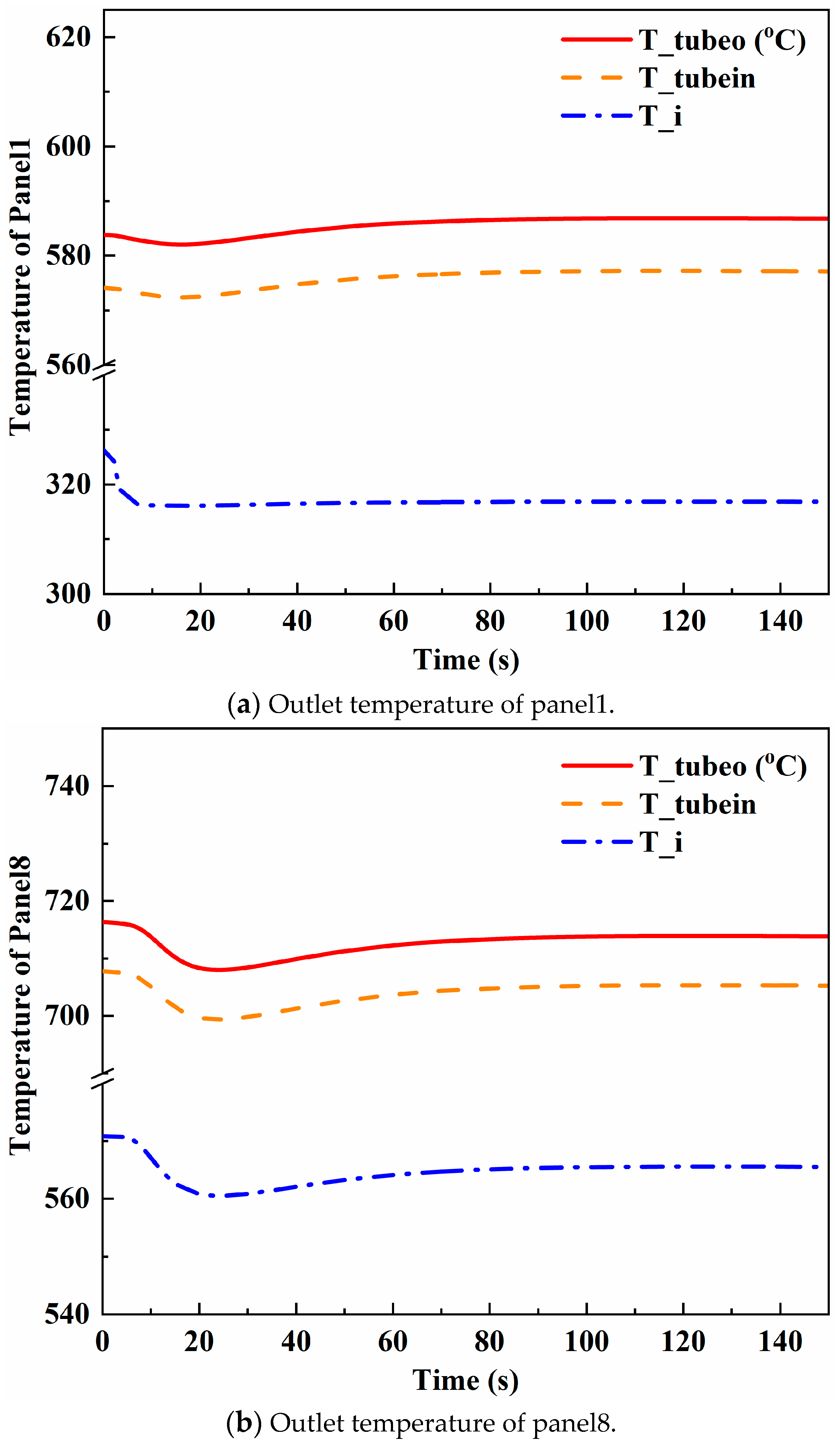
3. Results with Analysis

For the intermittency and volatility of solar energy, the receiver is exposed to fierce operation conditions. Its operation is closely related to its life span and the quality of the energy storage. The outlet temperature of the molten salt should be kept at the rated value to make sure decomposition does not happen, and the high quality steam is generated. Therefore, the safe operation is critical for the economic efficiency and security of the whole SPT plant. Many factors could affect its operation, such as DNI volatility, air temperature, pump failure, the stability of the control strategy, load variation, and the like. Their main disturbance factors are chosen to reveal the operation characteristics of the receiver.

At the beginning (0–2 s), the receiver is operated under the rated condition with the aim to verify the validity of the model. (v_amb = 4 m/s, T_amb = 20 °C, DNI = 800 W/m², $\dot{m}$_salt = 119.89 kg/s, T_{salt_in} = 290 °C). The boundaries of the three cases are restated (in

Table 3. Boundary conditions of each case.

Index	Simulation	DNI (W/m2)	Inlet Temperature (°C)	Mass Flux (kg/s)
A	DNI disturbance	---	290	---
B	Inlet temperature disturbance	800	290–280	---
C	Operation on cloudy day	---	290	---

). The symmetrical receiver can be observed, and it has two flow channels starting from the north and ending in the south. To adjust the temperature of the working fluid under consistent changing environment, the temperature control strategy is introduced. By regulating the mass flux of the working fluid according to the variation of the heat flux collected by the heliostat field, the temperature of molten salt is controlled. The heat transfer characteristics and the response curves of the panels in the beginning and the end are displayed as representatives. To make sure the temperature of the molten salt is unchanged after the regulation, the simulation time is 200 s. But only the data between 0–150 s are selected as a representative, the remainder is the same.

3.1. Case A. DNI Disturbance

3.1.1. Step DNI Disturbance Influence

The DNI dropped suddenly at 2 s (relative time) when the receiver operated at rated condition, from 800 to 600 W/m², with other variables being held constant. The outlet temperatures restored due to the temperature control strategy. The 0.1 s time step was selected for the calculation. The outlet temperatures of panel1 and panel8 are displayed in Figure 5.

The tube wall temperature drops dramatically when DNI drops. Because of the thermal lag, the temperature of the molten salt decreases slowly and the adjustment of the control strategyis made. By comparing the temperature of the tube wall and the molten salt, it can be seen that the influence of DNI on the tube wall is more obvious than the molten salt in the first panel (in Figure 5a). It takes around 110 s for the control strategy to adjust the molten salt temperature to the calibration value (565 °C). As can be seen in Figure 5b, it takes more time (around 130 s) for the last panel. The target of the control strategy is to stabilize the molten salt outlet temperature around 565 °C; therefore, its temperature and the temperature of the tube wall is stabilized after the temperature accommodation with DNI remains constant. The temperature difference of the last panel (5.9 °C) is smaller than that of the first panel (6.05 °C), which means the heat transfer effect of the first panel is better, and the tangential thermal stress of the first panel is higher than the last one according to Equation (14).

The conclusion can be made from the results that the temperature control strategy can levelize the DNI disturbance in a short period (in around 130 s). DNI perturbation can cause larger temperature variation of the tube wall (around 82 °C), rather than that of the molten salt (around 63 °C), when the DNI drops from 800 to 600 W/m², and temperature change of panel8 is larger than that of the first panel. The thermal stress is reduced for the reduction of temperature fluctuation. The time delay for thermal inertia in the last panel is more obvious than the previous panels by the observation of the trough of the response curves.

3.1.2. The Influence of Clouds Covering in a Short Period

During the operation of an SPT, clouds may appear upon the sky of the plants. To simulate the process of the receiver operation when clouds passed by, the following experiment with continuous DNI disturbance is launched. DNI decreases gradually from 800 to 600 W/m² in 10 s, then increases to 800 W/m² gradually at 25 s, as shown in Figure 6a. The DNI disturbance works from the 2 to 25 s.

The outlet temperature of molten salt restored to the rated value (565 °C) by temperature accommodation when disturbance appeared. Compared with the response curves in Figure 6b, it takes more time (around 140 s) to restore to the rated temperature because the DNI disturbance lasts longer. The temperature fluctuation of the molten salt and tube wall is around 45 and 58 °C (Figure 6c), respectively, which is smaller than the temperature variation of the DNI step disturbance experiment. The temperature fluctuation range is 20 °C shorter. For the help of reciprocating DNI disturbance, thermal inertia can levelize temperature fluctuation. Therefore, the covering of the cloud for a short period is better than a long period. The robustness of the control strategy is verified.

3.2. Case B. Molten Salt Inlet Temperature Disturbance

As the plants grow older, insulation failure of the receiver could appear, including that of the delivery ducts. In addition, the inhomogeneity of temperature distribution in tanks is also a factor of temperature interference. Consequently, the molten salt inlet temperature in the receiver could drop, which proposes a challenge for the control strategy. To confirm the effectiveness of the control strategy, and the response properties of the receiver, the step disturbance of the molten salt inlet temperature is chosen. At 2 s, the molten salt inlet temperature has a 10 °C drop from 290 °C.

As the perturbation starts from the molten salt, the outlet temperature of molten salt drops first (Figure 7a). Heat transfer increases when the temperature difference between the tube wall and molten salt increases, which is the reason for the temperature drops of the tube wall. The temperature drops of the molten salt and tube wall are 5 and 8 °C, respectively (Figure 7a). The temperature variation in the last panel is reduced for the thermal inertia and the temperature control strategy. Cold salt is heated to the rated value (565 °C) by the temperature control and stabilized when it comes out of the receiver.

3.3. Case C. The Influence of the Real-Time DNI during a Day

In this section, the temperature control strategy of the receiver is tested during the operation during a period of a cloudy day. In order to save the calculation cost, a period from 9:30 to 11:30 am is selected for the test, which is illustrated in the box with the blue line in Figure 8a.

The response curves can be described in Figure 8b,c. In general, the response curves are smooth except for the sharp spike at 11:15 am. It can be that the DNI increases swiftly from 400 to 835 W/m² at 11:15 am in Figure 8a. Huge thermal stress is generated at each panel. In Figure 8b, the temperature of the tube wall of panel1 reaches to 800 °C, and in panel 8, it reaches to 1100 °C (in Figure 8c), which can cause damage to the tubes. The molten salt temperature in panel8 is over 700 °C. The high temperature can cause the pyrolysis of the molten salt. This case should be escaped during the operation of the receiver for its safety. In Figure 8d, the actions of the control system are stated. By the flow rate regulation of the control strategy, the molten salt temperature is kept well within reasonable bounds around the rated value (565 °C). The molten salt outlet temperature is not only the object of the control strategy but also the feedback signal of the controller. In view of the feedback signal and the feedforward signal (the molten salt mass flux), the controller sends commands to the molten salt pump. Under the DNI disturbance from 9:30 to 11:10 am, the temperature is stabilized at the rated value very well. However, the control strategy is disabled for several minutes under a violent swing during 11:13 to 11:15 am. Therefore, a more accurate control strategy should be applied, such as a double-pulse control system and a three-impulse control system.

The influence of the two main disturbance factors, including DNI and the molten salt inlet temperature, are investigated. Step disturbance of DNI is imposed on the model to explore the response properties of the molten salt external receiver against the unstable environment. DNI changes gradually in a short period during the passage of a cloud. So the reciprocating disturbance of DNI is chosen to study the heat transport properties of the receiver. The DNI data of a typical cloudy day is acquired in Figure 8a. The validity of the temperature control strategy is verified from 9:30 to 11:30 am. The results obtained will contribute to the SPT control strategy formulation.

4. Conclusions

A 100 MW external receiver is designed based on the design criteria of the molten salt cylindrical receiver. A one-dimension comprehensive model is established accordingly. The temperature control strategy is applied to the receiver to make sure the outlet temperature of molten salt stabilized at the rated value. The control strategy is tested under DNI disturbance and molten salt inlet temperature disturbance. The robustness of the control strategy is displayed, and the emergency case is pointed out. The results obtained will contribute to the control strategy formulation of an SPT plant. The conclusions can be summarized below.

(1) The DNI perturbation has a more direct impact on the tube wall rather than the molten salt. The temperature variation of the last panel is larger than the previous ones. The temperature variation of the tube wall is greater than the molten salt under the disturbance of DNI and molten salt inlet temperature. The passage of a cloud in a short period is better than a long period covering of a cloud, which helps reduce the temperature fluctuation. The temperature difference in the former panels is higher than the later ones, which have a higher heat transfer efficiency. Therefore, the tangential thermal stress of the former panels is higher than the last ones.

(2) The thermal inertia of the receiver is demonstrated, and the time constant of the receiver is acquired. The temperature drops can reinforce the heat transfer in the absorber tubes. The thermal inertia has the function of reducing temperature fluctuation. Compared with the DNI disturbance, its influence on the receiver is more mitigatory.

(3) The validity of the temperature control strategy is verified. The response curves of the receiver under disturbances have stated the robustness of the control strategy. Generally, the molten salt outlet temperature is controlled well under the condition of DNI step disturbance, inlet temperature step disturbance, cloud passage, and the real-time DNI variation. However, control strategy failure appears for several minutes under large fluctuation of DNI, which is harmful to the receiver and molten salt. The over-temperature case appears during the typical cloudy day operation. A more accurate control strategy is recommended, such as a double-pulse control system and a three-impulse control system.

References

1. Rashid, K.; Mohammadi, K.; Powell, K. Dynamic simulation and techno-economic analysis of a concentrated solar power (CSP) plant hybridized with both thermal energy storage and natural gas. J. Clean. Prod. 2020, 248, 119193. [Google Scholar] [CrossRef]
2. Hsieh, I.Y.L.; Pan, M.S.; Chiang, Y.M.; Green, W.H. Learning only buys you so much: Practical limits on battery price reduction. Appl. Energy 2019, 239, 218–224. [Google Scholar] [CrossRef]
3. Budischak, C.; Sewell, D.; Thomson, H.; Mach, L.; Veron, D.E.; Kempton, W. Cost-minimized combinations of wind power, solar power and electrochemical storage, powering the grid up to 99.9% of the time. J. Power Sources 2013, 225, 60–74. [Google Scholar] [CrossRef] [Green Version]
4. Heide, D.; Greiner, M.; Bremen, L.; Hoffmann, C. Reduced storage and balancing needs in a fully renewable European power system with excess wind and solar power generation. Renew. Energy 2011, 36, 2515–2523. [Google Scholar] [CrossRef] [Green Version]
5. Sánchez-González, A.; Rodríguez-Sánchez, M.R.; Santana, D. Allowable solar flux densities for molten-salt receivers: Input to the aiming strategy. Results Eng. 2020, 5, 100074. [Google Scholar] [CrossRef]
6. Wang, W.Q.; Qiu, Y.; Li, M.J.; He, Y.L.; Cheng, Z.D. Coupled optical and thermal performance of a fin-like molten salt receiver for the next-generation solar power tower. Appl. Energy 2020, 272, 115079. [Google Scholar] [CrossRef]
7. Ying, Z.; He, B.; Su, L.; Kuang, Y.; He, D.; Lin, C. Convective heat transfer of molten salt-based nanofluid in a receiver tube with non-uniform heat flux. Appl. Therm. Eng. 2020, 181, 115922. [Google Scholar] [CrossRef]
8. Du, B.C.; He, Y.L.; Zheng, Z.J.; Cheng, Z.D. Analysis of thermal stress and fatigue fracture for the solar tower molten salt receiver. Appl. Therm. Eng. 2016, 99, 741–750. [Google Scholar] [CrossRef]
9. Yang, M.; Yang, X.; Yang, X.; Ding, J. Heat transfer enhancement and performance of the molten salt receiver of a solar power tower. Appl. Energy 2010, 87, 2808–2811. [Google Scholar] [CrossRef]
10. Yu, Q.; Fu, P.; Yang, Y.; Qiao, J.; Wang, Z.; Zhang, Q. Modeling and parametric study of molten salt receiver of concentrating solar power tower plant. Energy 2020, 200, 117505. [Google Scholar] [CrossRef]
11. Zhang, Q.; Wang, Z.; Li, X.; Li, Z.; Li, J.; Liu, H.; Ruan, Y.; Xu, L. Preliminary discussion on test method for time constant of molten salt receiver based on two-lumped-elements model. Sol. Energy 2020, 195, 552–564. [Google Scholar] [CrossRef]
12. Zhang, Q.; Li, X.; Wang, Z.; Zhang, J.; El-Hefni, B.; Xu, L. Modeling and simulation of a molten salt cavity receiver with Dymola. Energy 2015, 93, 1373–1384. [Google Scholar] [CrossRef]
13. Zhang, Q.; Li, X.; Wang, Z.; Li, Z.; Liu, H. Function testing and failure analysis of control system for molten salt receiver system. Renew. Energy 2018, 115, 260–268. [Google Scholar] [CrossRef]
14. Fernández-Torrijos, M.; Sobrino, C.; Marugán-Cruz, C.; Santana, D. Experimental and numerical study of the heat transfer process during the startup of molten salt tower receivers. Appl. Therm. Eng. 2020, 178, 115528. [Google Scholar] [CrossRef]
15. Li, Z.; Zhang, Q.; Wang, Z.; Li, J.; Ruan, Y. Numerical and experimental study of solidification dangers in a molten salt receiver for cloudy conditions. Sol. Energy 2019, 193, 118–131. [Google Scholar] [CrossRef]
16. Zhang, Q.M. Study and Design of Heat Transfer Characteristics of Molten Salt Receiver in Solar Tower Power Plant; Zhe Jiang University: Zhejiang, China, 2014. (In Chinese) [Google Scholar]
17. Zhang, Q.; Cao, D.; Ge, Z.; Du, X. Response characteristics of external receiver for concentrated solar power to disturbance during operation. Appl. Energy 2020, 278, 115709. [Google Scholar] [CrossRef]
18. Dong, X.; Bi, Q.; Yao, F. Experimental investigation on the heat transfer performance of molten salt flowing in an annular tube. Exp. Therm. Fluid. Sci. 2019, 102, 113–122. [Google Scholar] [CrossRef]
19. Siebers, D.L.; Kraabel, K.J. Estimating Convective Energy Losses from Solar Central Receivers; Sandia National Laboratories: Albuquerque, NM, USA, 1984. [Google Scholar]
20. Wagner, M. Simulation and Predictive Performance Modeling of Utility-Scale Central Receiver System Power Plants; University of Wisconsin-Madison: Madison, WI, USA, 2008. [Google Scholar]
21. Eloy, C.; Doare, O.; Duchemin, L.; Schouveiler, L. A Unified Introduction to Fluid Mechanics of Flying and Swimming at High Reynolds Number. Exp. Mech. 2010, 50, 1361–1366. [Google Scholar] [CrossRef]
22. Bradshaw, R.W.; Dawson, D.B.; Rosa, D.L.; Gilbert, R.; Goods, S.H.; Hale, M.J.; Jacobs, P.; Jones, S.A.; Kolb, G.J.; Pacheco, J.E.; et al. Final Test and Evaluation Results from the Solar Two Project; National Renewable Energy Laboratory (NREL): Golden, CO, USA, 2002. [Google Scholar]
23. Sanchez-Gonzalez, A.; Rodriguez-Sanchez, M.R.; Santana, D. Aiming strategy model based on allowable flux densities for molten salt central receivers. Sol. Energy 2017, 157, 1130–1144. [Google Scholar] [CrossRef]
Figure 1. The flowchart of the external receiver structure.
Energies 14 00340 g001
Figure 2. Schematic of absorbing tube model discretization and element energy balance.
Energies 14 00340 g002
Figure 3. Calculation flow chart of the model.
Energies 14 00340 g003
Figure 4. Validation of temperature distribution along the flow direction.
Energies 14 00340 g004
Figure 5. Influence of Step DNI disturbance (800–600 W/m2).
Energies 14 00340 g005aEnergies 14 00340 g005b
Figure 6. Influence of reciprocating DNI disturbance (800–600–800 W/m2).
Energies 14 00340 g006aEnergies 14 00340 g006b
Figure 7. Influence of molten salt inlet temperature disturbance.
Energies 14 00340 g007
Figure 8. Response curves on a cloudy day under temperature control strategy.
Energies 14 00340 g008aEnergies 14 00340 g008b