Abstract
The subject of the dynamic analysis presented in the article is the linear drive system with a timing belt utilized in the automatic device for polymer composite belt perforation. The analysis was carried out in two stages. In the first stage, the timing belt was modeled with all the relevant dynamic phenomena; subsequently, the tension force of the belt required for the correct operation of the belt transmission was determined. The necessary parameters for belt elasticity, vibration damping, and inertia are based exclusively on the catalog data provided by the manufacturer. During the second stage, equations of motion were derived for the designed drive system with a timing belt, and characteristics were identified to facilitate the optimal selection of electromechanical drives for the construction solution under analysis. The presented methodology allows for designing an effective solution that may be adapted for other constructions. The obtained results showed the influence of the kinematic parameters on the motor torque and proved the importance of reducing the mass of the components in machines that perform high-speed processes.
1. Introduction
In mechatronic design, the model which can focus on either functional or structural form is a very important tool [1]. By juxtaposing these two models, we are able to examine designs at an early stage [2]. The use of mathematical models to describe the dynamics in a given device not only improves the control process of the machine (e.g., choosing the settings for control systems) but also makes it possible to verify its structural features [3,4,5]. The main challenge is usually the determination of model parameters for the basic mechanical components used in machine construction, such as guides, couplings, bearings, or belt transmissions [6,7]. Manufacturers provide a lot of different information in their product catalogs, but determining or finding the necessary parameters describing elasticity, vibration damping or inertia for the machine components is challenging without experimental studies.
Multiple examples of modeling the dynamics of mechanisms and drive systems with flat belts, V-belts, or timing belts can be found in the literature. Shirafuji et al. [8] proposed and analyzed a novel mechanism used for locking the flat belt and derived analytically the relationship between the tensile force and the frictional force. Balta et al. [9] modeled the speed losses in V-ribbed belt drives and found the correlation between the pulley size and the belt slip. Callegari et al. [10] tested the dynamic behavior of the timing belt transmissions in terms of acoustic radiation. Long et al. [11] analyzed the dynamic performance of the timing belt and presented the influence of the tensioner design and belt pre-tension on the dynamic belt tension. Domek et al. [12] modeled the wear of the timing belt pulley, while Hamilton et al. [13] presented the combination of the computer-based analytical simulation methods coupled with statistical tools to predict the timing belt life. Merghache and Ghernaout [14] focused on studying the heat transfer through the belt transmissions concerning different rotational speeds, engine torque, and setting tension. The computational methods were also used to model the belt passage by the driving drum [15] or to obtain the belt movement characteristics [16]. As can be observed in the above-mentioned research publications, the pre-tension of the belt affects the dynamic properties of the belt the most and should be precisely tested in order to gain the most effective exploitation parameters. Additionally, none of the papers presented above has been concerned with linear drive systems with timing belts. For that reason, before determining the dynamics model of the whole drive system, the focus should be put on modeling the belt itself.
The dynamics of the drive systems have an influence on the power consumption of the designed machine. The rational design of the work drive system may greatly reduce the torque or the force, which has to be generated in order to properly perform the technological process [17]. If the machine is supplied with an electric motor, this value will have an impact on the power consumption of the machine. Electric motors are designed to work in the range between 50–100% of the rated load [18]. Below this value the power factor decreases sharply [19], resulting in inefficient power consumption of the electric device. This implies that performing a complex dynamic analysis of the designed structure may lead to improvements in the energetic efficiency of the device. Based on its results, it is possible to select a motor power very close to the real rated load. Of course, the method of controlling and using proper motor drivers or regulators will also have an effect on power consumption [20]. The dynamic model of the drive system can be also useful in selecting the parameters of the applied PI or PID regulators, which will increase the precision of positioning and prevent the occurrence of resonance.
This article presents the methodology for modeling the dynamics of the designed device based on the catalog data and geometric parameters that are available at the design stage, using linear drive systems with timing belts employed in automatic devices for polymer composite belt perforation as an example. This approach makes it possible to design an effective device structure and analyze it at the design stage. In addition, the article provides the methodology of modeling the timing belt with a view to analyze aspects of drive system dynamics. All these aspects can be used to improve the efficiency and power consumption of the designed electric device.
2. Materials and Methods
The object of research is the automatic device for composite polymer belt perforation (Figure 1) [21]. It features two mirrored perforating heads and one separated working drive unit. The pressure plate connected with the working drive actuators presses on one or two heads at the same time, affecting the motion of the head-punch plate and cutting the hole in the belt using the punch and die. Both punching dies move along a shared linear die, whereas the working drive system has its own guiding system. Since both of the punching dies have significant mass and the process works at rather high speed and acceleration, the inertia will have a crucial influence on selecting the proper drive [22]. Each of those subassemblies is driven by an individual, linear drive system with a timing belt spanning between the driven and idle wheel systems. Each of the belts features a bolt tensioner mechanism.
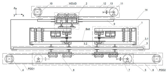
Figure 1.
Schematic of the belt perforation device in a configuration using a punch and a die [23]: 1—punching die, 2—work drive unit (WDU), 3—punching die guide, 4—drive wheel assembly for punching die drive, 5—driven wheel assembly punching die drive (PDD), 6—lower toothed belt, 7—lower belt tensioner, 8—punching die drive mount, 9—WDU guide, 10—WDU drive wheel assembly, 11—WDU driven wheel assembly, 12—upper toothed belt, 13—upper belt tensioner, 14—frame, Belt—perforated belt, PDDi—i-th punching die drive system, WDUD—WDU drive system.
To design an effective automatic device for belt perforation, it is crucial to determine the peak torque, which will be used to select an electric motor and transmission. In the case of the mechatronic applications, this procedure should be supported by the dynamic model of the mechanical structure [24]. By analyzing the stiffness, inertia, and damping of the machine, it is possible to perform the parameter optimization [25], which results in designing effective mechatronic devices.
The analysis was carried out in two stages. In the first stage, the timing belt was modeled with all the relevant dynamic phenomena; subsequently, the tension force of the belt required for the correct operation of the belt transmission was determined. The necessary parameters for belt elasticity, vibration damping, and inertia are based exclusively on the catalog data provided by the manufacturer. During the second stage, equations of motion were derived for the designed drive system with a timing belt using the general form of Lagrangian equations of the second kind. Then, the characteristics were identified to facilitate the optimal selection of electromechanical drives for the design solution under analysis.
3. Results
3.1. Modelling the Timing Belt Dynamic Behavior
In order to correctly model the operation of the linear drive system designed on the basis of a toothed belt, one should begin with modeling the belt itself (Figure 2).
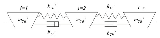
Figure 2.
Model of the toothed belt within the drive system.
Assuming that the tooth i = 1 is acting as support, the tensile force F resultant from the drive torque TM of the belt wheel with diameter D is applied to the tooth i = z, where z is the number of belt teeth on the section with length equal to the distance between the belt wheel axles a; hence, the toothed belt can be modeled as a system comprising z − 1 systems, including body-spring-damper (m-k-b) with parameters as provided on Figure 2, connected in series [26,27].
For a system comprising sets of units connected in series, the displacement of the entire system is equal to the sum of displacement of every constituent, whereas each component is affected by an identical force equal to the global load. Within the m-k-b system, the constituents are connected in parallel, i.e., the displacement of each component is the same, whereas the force is distributed on all the components proportionally to displacement (for the spring), velocity (for the damper), and acceleration (for the body). As the structure of the belt is uniform along its entire length, the coefficients of elasticity kTB’, coefficients of damping bTB’ and single unit weights mTB’ are identical for each m-k-b system.
If the first link is immobilized, and each system is displaced equally by the value x’ the displacement of the solid body i is equal to . Assuming the system number including body , it can be described with the following set of equations:
After summing the equations, we arrive at:
After dividing both sides of the equation by (z − 1) and introducing the dependency (3), the following characteristic is obtained (4).
Applying the replacement model as a single system of body-spring-damper with parameters mTB, kTB, and bTB, we arrive at the following dynamic equation:
Considering that the weight of the entire belt on the examined section can be calculated with Equation (6), we receive the following substitute parameters for the model as provided in Equations (7)–(9).
3.2. Dynamic Analysis of the Timing Belt Linear Drive Systems
The above model of the toothed belt is used in the dynamic models of linear drive systems for perforating heads as well as the working drive unit. All three systems are implemented in an analogous manner to Figure 3 and Figure 4. In these systems, the moving component is rigidly connected via toothed plates to the toothed belt which spans between the two toothed belt wheels. The analyzed component travels along a profiled linear guide on carriages with rolling components. The driven wheel uses a brushless direct current drive (BLDC), its shaft is connected to the wheel shaft via the dog clutch with a polyurethane insert.
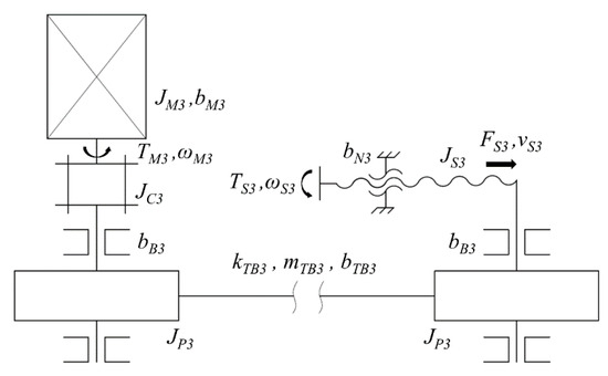
Figure 3.
General schematic of the linear drive system with a toothed belt.
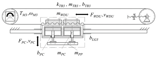
Figure 4.
Schematic of the linear drive system of the work drive unit (WDU) [23].
To ensure the correct operation of the presented linear drive system, correct belt tensioning is required. With a too-low initial belt tension, the teeth of the idle belt section collide or overlay with the teeth of the wheel and increased surface wear occurs due to friction as teeth are engaged. Furthermore, forced breakage of the belt may occur due to excessive elongation caused by complete overlap of teeth. On the other hand, excessive belt tension causes a high load on shaft bearings, reduces transmittable power, and increases wear of the belt teeth. It is therefore critical to select the correct belt tensioning for the designed system. The tensioning in the current design is achieved with an adjustable bolt mechanism (Figure 3 and Figure 4).
In order to apply the simplifying solutions, in which the relative belt displacement in relation to the fastened head is 0, belt tensioning with force Ft, which fulfills the following inequality resultant from d’Alembert’s principle, is required:
To maintain the rigidity of the coupling, the force resulting from the belt’s flexibility should compensate for the inertial force of the moving component:
As the peak value of force Ft is known, we are able to calculate the displacement value to be affected on the belt to ensure correct tensioning:
Once this value is known, the belt tensioning process, together with controlling the correctness of tensioning, can be easily automated. With known parameters of the thread used in the bolt tensioning mechanism (fine thread M10×1 with pitch diameter d2 = 9.35 mm and pitch Pt = 1 mm) and the coefficient of friction between the bolt and the nut (μ = 0.2), the moment of friction between the bolt and the nut can be calculated from the equation:
where:
- lead angle of helix ,
- apparent angle of friction .
The selection of the toothed belt with the selected pitch is carried out on the basis of displaced component and maximum assumed acceleration. The design assumes the mass of a single perforating head mPD = 90 kg and the mass of the work drive system mWDU = 50 kg. Based on the catalog data, AT10 belts (Pbelt = 10 mm) with widths 32 mm and 25 mm, respectively, (Figure 5) were selected for the drive systems.
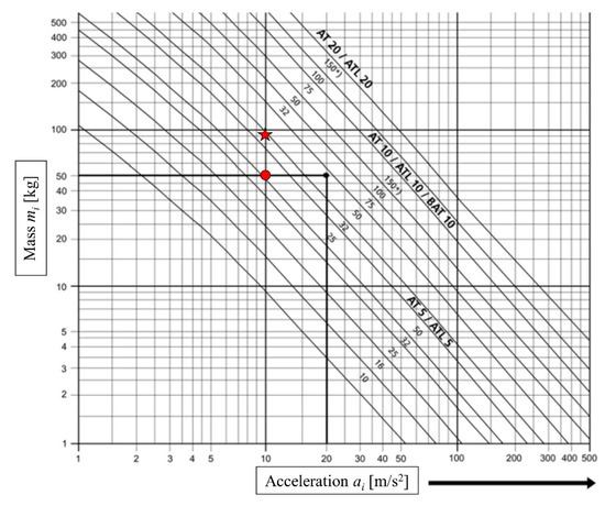
Figure 5.
Methodology of the selection of the toothed belt on the basis of the manufacturer’s catalog data [28]: red dot and star represents the combination of mass and acceleration for WDUD and PDD respectively.
In order to determine the model parameters of the belt as an m-k-b system, the manufacturer data provided in the catalog were used as provided in Figure 6 and Figure 7. For the purpose of calculations, it is further required to identify the distance between the belt wheel axles a, which for the working drive system is 1245 mm and for the perforating head drive is 795 mm. It is used to calculate the number of belt teeth on the examined section (Equation (14)), as well as the actual mass of the belt mbelt (Equation (15)), which is used to determine the substitute mass mTB according to the Equation (7).
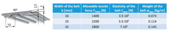
Figure 6.
Belt catalog data including weight, and elasticity [28].
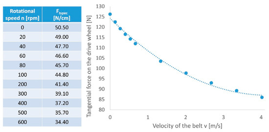
Figure 7.
The catalog data for the belt regarding the influence of rotation speed n (rpm) on the allowable distributed load on a single tooth Ftspec (N/cm) together with the characteristic of the tangential force as a function of the belt linear velocity for belt wheel diameter D = 128 mm and belt width W = 25 mm [28].
Using the data in the manufacturer’s catalog, it is possible to calculate maximum belt deformation ε (Equation (16)), and after multiplying it by the distance between the wheel axles, we obtain the threshold belt displacement value x. Dividing the allowable tensioning force value FTadm by displacement x, we obtain belt elasticity kTB.
The major challenge is in determining the b coefficient, which defines the rheological characteristics of the belt. To this end, the information on the maximum distributed load per one tooth for different rotation speeds of the driven wheel is required. This information is transformed into the characteristics of the tangential force as a function of the belt linear velocity Ft(v).
The decreasing allowable force load on the belt is a consequence of the allowance established from process dynamics. Therefore, if the value Ft (v = 0) = Ft0 is assumed to be static and by calculating the difference between the obtained force value and static force Ft0 for every point of measurement, we receive the characteristic curve Fb(v). Approximating the characteristic curve to a linear function, we arrive at the belt damping constant bTB (Figure 8).
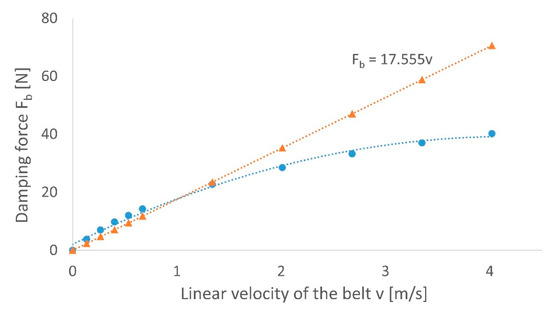
Figure 8.
Modeling the coefficient of damping bTB for the toothed belt.
Assuming the bolt acceleration is equal to 0.1 m/s2 and maximum bolt speed 5 mm/s, we arrive at the maximum force value Ftpeak = 505.1 N. Therefore, the belt is to be tensioned until the displacement value by 1.15 mm is achieved. Calculating this as the torque for the tensioning bolt, one needs to use a drive with nominal torque 0.63 Nm.
To establish the equations of motion for the linear drive system, the general form of Lagrangian equations of the second kind were used together with the diagrams provided in Figure 3 and Figure 4.
The kinetic energy in the system under examination for the working drive system is expressed with the below equation:
Considering the ratio of the belt transmission ip = 1 and identical moments of inertia for both belt wheels JP3 = JP3′ together with the dependency between linear and angular velocity , as well as vS3 = 0 due to correct belt tension, we arrive at the following:
Considering that all the constituents of the analyzed system move along a horizontal axis and the height of their centers of gravity remain unchanged during motion, the potential energy does not include the energy originating from gravity, only the elasticity of the toothed belt:
If therefore , as well as the derivative .
To describe the mechanical losses in the device, it is required to calculate the power of dissipation :
Considering the kinematic correlations as described above and the transmission ratio together with the identical bearing of both belt wheels we arrive at:
Generalized force: .
The dynamic equation for the examined system has the following form:
Calculating the drive torque of the BLDC motor, we receive the characteristic curve :
The values of moments of inertia together with the masses of individual system components were derived from the manufacturer’s catalog or the CAD software for 3D modeling. In order to model the coefficient of damping bM3, which defines mechanical losses resulting primarily from friction, the catalog data on drive efficiency were used.
Regarding roller guides employed in the design, the guide frictional resistance may constitute only 1/20 to 1/40 of the frictional resistance of a comparable slide rail. This is observable in particular for static friction, which is significantly lower for the roller bearing. Moreover, the difference between the static and dynamic friction is very low; therefore, the problem of the so-called stick-slip effect is not present. Due to such low friction, relatively low powered drive motors are suitable for the guides. The friction resistance of linear guides may vary within a specific range due to load, initial tension, lubricant viscosity, the number of seals, and other factors. The frictional resistance of the guide can be calculated using a formula based on working load and packing friction. Generally speaking, the coefficient of friction for ball-type guides is 0.002–0.003 (without packing), and for roller type guides is 0.001–0.002 (without packing) [29]. Therefore, this constituent can be omitted in the model, but in the literature, we can find some models to determine the dynamics of such machine components [30]. However, for slide rails, these losses need to be accounted for.
Similar phenomena are observed in the case of roller bearings. The breakaway torque can be determined based on manufacturer catalog data [31]; however, its value is low in comparison to resistances resulting from inertia.
In order to determine the torque parameters of motors M1 and M2 driving the perforating heads, the model developed above was also utilized. the only difference was in regard to the generalized force value Qj, which was calculated using the principle of virtual work, including an additional resistance force caused by the belt adhering to the perforating head or uncut strands being caught on the punch. The drive torque of the motor should enable continued operation of the process in case such resistances occur (sever the strand or separate the belt from the head).
The design for both drive systems is identical, therefore a single dynamic equation was used for its mathematical description:
Based on the equations of motion 26 and 28, example drive characteristics for various accelerations (Figure 9 and Figure 10) and velocities (Figure 11 and Figure 12) were derived. To obtain the characteristic which will enable selecting the proper drive for chosen kinematic parameters, the peak torque values were compared with the rotational acceleration and presented in Figure 13.
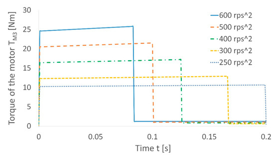
Figure 9.
Characteristic curves of the WDU drive motor torque for various rotational acceleration ε and maximum rotational speed ω = 3000 rev/s.
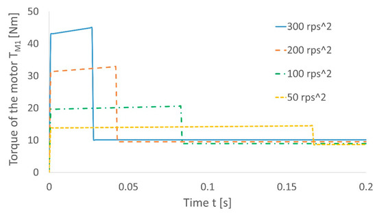
Figure 10.
Characteristic curves for the perforating head drive motor torque for various rotational acceleration ε and maximum rotational speed ω = 500 rev/s and assuming uncut strand resistance force of FR = 50 N.

Figure 11.
Characteristic curve of the WDU drive motor torque for rotational acceleration ε = 500 rev/s2 and various maximum rotational speed ω.
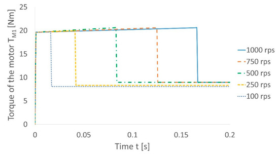
Figure 12.
Characteristic curve for the perforating head drive motor torque for rotational acceleration ε = 100 rev/s2 and various maximum rotational speed ω and assuming uncut strand resistance force of FR = 50 N.
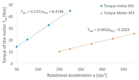
Figure 13.
The influence of the rotational acceleration ε on the peak head/WDU drive motor torque for maximum rotational speed ω = 500 rev/s (for head drive) or ω = 3000 rev/s (for WDU drive).
4. Discussion
Based on the obtained results presented in the previous section, the analysis of the influence of the kinematic parameters (rotational speed and acceleration) on the selected motor torque can be performed. By combining these results, it is possible to calculate the amount of energy used in the acceleration phase, which can be used to evaluate the power consumption of the machine.
As can be observed in Figure 9 and Figure 10, by increasing the acceleration and maintaining constant maximal rotational speed, the maximum torque rises sharply. The significance of this growth is caused by the inertia of the mass of the punching dies. After achieving the maximum constant speed, the static torque falls down to 10 times lower values (for the greatest value of acceleration). This shows the importance of reducing the mass of the components in machines that perform high-speed processes. Comparing both analyzed drive systems, the static torque is much higher for a drive of the punching die than for the drive of the work driving unit. It is caused by the drag from the uncut fibers of the perforated belt, which was taken into consideration in the model derivation. If we analyze the energy used in the acceleration phase for both cases (Figure 14), which can be estimated as a product of peak torque Tmax, maximum angular velocity ωmax, and time of acceleration ta (Equation (29)) [32], it remains almost constant, but for very low acceleration (below 100 rev/s2), it starts to grow. This implies that working at very low speeds is not recommended, taking into account the power consumption of the machine, especially since it will require greater time to go the same positioning distance as for higher speeds.
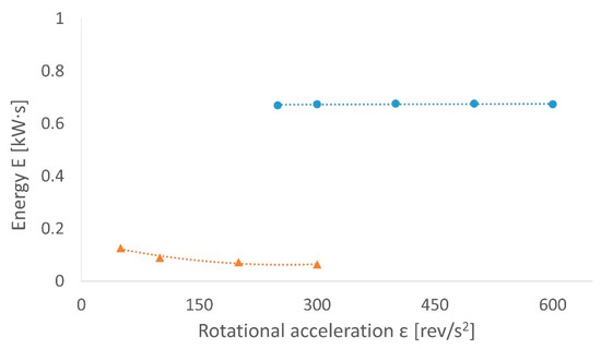
Figure 14.
The correlation between the consumed energy in the acceleration phase and the rotational acceleration ε for a constant maximum rotational speed ω for WDU (orange) and perforating head (blue) drives.
For varying maximum rotational speed (Figure 11 and Figure 12), the value of the peak torque is always the same regardless of the speed. However, it affects the time of acceleration as it decreases when the torque value gets lower. If we analyze the energy used during the acceleration phase in the function of maximum rotational speed for a constant rotational acceleration, for both discussed drive units (Figure 15), the non-linear correlations are obtained. It implies that the power consumption can be reduced by rational limitation of the positioning velocity. On the other hand, it may greatly increase the time of operation, which is a negative effect for high-speed processes.
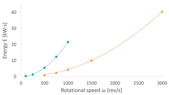
Figure 15.
The correlation between the consumed energy in the acceleration phase and the rotational speed ω for a constant maximum rotational acceleration ε for WDU (orange) and perforating head (blue) drives.
Although it was proved that the rotational acceleration ε does not have a significant influence on energy consumption, it still has a crucial impact on the peak motor torque. As can be observed in Figure 13, in both cases, we obtain a linear positive correlation. Taking into consideration both power consumption and torque necessary to put the mass into motion, it is advantageous to select the acceleration which lies in the middle of the analyzed range to find the compromise (in the case of the described device, approx. 200 rev/s2).
If we discuss the application of the presented model, the methodology of its derivation and obtained characteristics, aside from the torque and power consumption estimation, it can be used to determine the value of the resistance force caused by the belt adhering to the perforating head or uncut strands being caught on the punch. The value of the resistance force can be determined by measuring the torque on the drive and comparing the obtained characteristics based on the dynamics analytical model. Additionally, it can be also used to determine the parameters of the positioning regulator for selected kinematic parameters. As was stated in the introduction, by performing such analysis for a drive selection, it is possible to almost fully exploit the motor and avoid working with the load below 50% of the rated power. It will also enable designing lighter and more effective solutions.
5. Conclusions
The conclusions of the presented research can be divided into two groups based on their impact: the general ones connected with the presented methodology of modeling and its application and the detailed ones connected with the analyzed design solution.
First of all, it is worth mentioning that the presented methodology of modeling facilitates the analysis of dynamics in the designed device based on the information made available by manufacturers in product catalogs. It can therefore be successfully employed in the design process of mechatronic devices in order to develop an effective solution with optimal drive systems, without oversizing the structure and working with a load below 50% of the rated power, which leads to lower efficiency.
Secondly, the analysis of the timing belt behavior showed the significance of determining the suitable belt tensioning in the belt transmission, which can be achieved based on the dynamic model as presented in the paper.
Based on the obtained results, it was shown that although using greater rotational acceleration will cause a significant increase of the torque generated by the motor (to values even ten times greater than the static torque), which highlights the importance of minimizing the inertia of the mechanical parts, especially the ones used in high-speed process machines. However, limiting the acceleration too much may lead to greater power consumption. Although the greater velocity of positioning does not affect the peak torque, it will increase the power consumption in the acceleration phase, but due to the shorter positioning time, it may still have a positive effect on overall exploitation. As discussed, selecting kinematic parameters is crucial and it is required to find the compromise without tending to neither maximization nor minimization.
Lastly, in the example of the linear drive system utilized in the automatic device for belt perforation, it was demonstrated that Lagrangian equations of the second kind are usable in the process of selecting the mechatronic device based on characteristics obtained from equations of motion. It may also have some additional applications, i.e., in the measurement methods for resistance force or to adjust the positioning regulator parameters. However, it can still be made more detailed e.g., by a more accurate description of the phenomenon of friction in the guides and bearings.
Author Contributions
Conceptualization, D.W. (Dominik Wojtkowiak) and K.T.; methodology, D.W. (Dominik Wojtkowiak) and K.T.; validation, D.W. (Dominik Wojtkowiak), K.T., D.W. (Dominik Wilczyński), J.G. and K.W.; formal analysis, D.W. (Dominik Wojtkowiak), K.T., D.W. (Dominik Wilczyński), J.G. and K.W.; investigation, D.W. (Dominik Wojtkowiak); resources, D.W. (Dominik Wojtkowiak); data curation, D.W. (Dominik Wojtkowiak), J.G. and K.W.; writing—original draft preparation, D.W. (Dominik Wojtkowiak); writing—review and editing, K.T. and D.W. (Dominik Wilczyński); visualization, D.W. (Dominik Wojtkowiak); supervision, K.T.; project administration, D.W. (Dominik Wojtkowiak); funding acquisition, K.T. All authors have read and agreed to the published version of the manuscript.
Funding
This research received no external funding.
Institutional Review Board Statement
Not applicable.
Informed Consent Statement
Not applicable.
Data Availability Statement
Data sharing not applicable.
Conflicts of Interest
The authors declare no conflict of interest. The funders had no role in the design of the study; in the collection, analyses, or interpretation of data; in the writing of the manuscript, or in the decision to publish the results.
References
- Pietrusiewicz, K. Projektowanie mechatroniczne. Projektowanie bazujące na modelach. Napędy Sterow. 2015, 11, 122–126. [Google Scholar]
- Heimann, B.; Gerth, W.; Popp, K. Mechatronika: Metody, Komponenty, Przykłady; Wydawnictwo Naukowe PWN: Warszawa, Poland, 2001. [Google Scholar]
- Vasylius, M.; Augustaitis, V.K.; Barzdaitis, V.; Bogdevicus, M. Dynamics of the air blower with gyroscopic couple. Acta Mech. Autom. 2008, 2, 95–98. [Google Scholar]
- Magdziak, Ł.; Malujda, I.; Wilczyński, D.; Wojtkowiak, D. Concept of Improving Positioning of Pneumatic Drive as Drive of Manipulator. Procedia Eng. 2017, 177, 331–338. [Google Scholar] [CrossRef]
- Wojtkowiak, D.; Talaśka, K.; Malujda, I.; Górecki, J.; Wilczyński, D. Modelling and static stability analyses of the hexa-quad bimorph walking robot. MATEC Web Conf. 2019, 254, 02029. [Google Scholar] [CrossRef]
- Zheng, Y.; Yang, Y.; Wu, R.-J.; He, C.-Y.; Guang, C.-H. Dynamic analysis of a hybrid compliant mechanism with flexible central chain and cantilever beam. Mech. Mach. Theory 2021, 155, 104095. [Google Scholar] [CrossRef]
- Song, N.; Peng, H.; Xu, X.; Wang, G. Modeling and simulation of a planar rigid multibody system with multiple revolute clearance joints based on variational inequality. Mech. Mach. Theory 2020, 154, 104053. [Google Scholar] [CrossRef]
- Shirafuji, S.; Matsui, N.; Ota, J. Novel frictional-locking-mechanism for a flat belt: Theory, mechanism, and validation. Mech. Mach. Theory 2017, 116, 371–382. [Google Scholar] [CrossRef]
- Balta, B.; Sonmez, F.O.; Cengiz, A. Speed losses in V-ribbed belt drives. Mech. Mach. Theory 2015, 86, 1–14. [Google Scholar] [CrossRef]
- Callegari, M.; Cannella, F.; Ferri, G. Multi-body modelling of timing belt dynamics. Proc. Inst. Mech. Eng. Part K J. Multi-Body Dyn. 2003, 217, 63–75. [Google Scholar] [CrossRef]
- Long, S.; Zhao, X.; Yin, H.; Zhu, W. Modeling and validation of dynamic performances of timing belt driving systems. Mech. Syst. Signal Process. 2020, 144, 106910. [Google Scholar] [CrossRef]
- Domek, G.; Kołodziej, A.; Wilczyński, M. Modelling of wear out of timing belt’s pulley. IOP Conf. Ser. Mater. Sci. Eng. 2020, 776, 012069. [Google Scholar]
- Hamilton, A.; Fattah, M.; Campean, F.; Day, A. Analytical Life Prediction Modelling of an Automotive Timing Belt. In SAE Technical Paper Series; SAE International: Warrendale, PA, USA, 2008. [Google Scholar]
- Merghache, S.M.; Ghernaout, M.E.A. Experimental and numerical study of heat transfer through a synchronous belt transmission type AT10. Appl. Therm. Eng. 2017, 127, 705–717. [Google Scholar] [CrossRef] [PubMed]
- Mikušová, N.; Millo, S. Modelling of Conveyor Belt Passage by Driving Drum Using Finite Element Methods. Adv. Sci. Technol. Res. J. 2017, 11, 239–246. [Google Scholar] [CrossRef]
- Yang, G.; Yang, L.; Cao, M. Simulation analysis of timing belt movement characteristics based on RecurDyn. Vibroeng. Procedia 2019, 22, 13–18. [Google Scholar] [CrossRef]
- Warguła, Ł.; Kukla, M. Determination of maximum torque during carpentry waste comminution. Wood Res. 2020, 65, 771–784. [Google Scholar]
- McCoy, G.A.; Douglass, J.G. Energy Efficient Electric Motor Selection Handbook; U.S. Department of Energy: Washington, DC, USA, 1996.
- Burt, C.; Piao, X.; Gaudi, F.; Busch, B.; Taufik, N.F.N. Electric Motor Efficiency under Variable Frequencies and Loads; Irrigation Training and Research Center Report No. R 06-004; Irrigation Training and Research Center: San Luis Obispo, CA, USA, 2006. [Google Scholar]
- Wieczorek, B.; Warguła, Ł.; Rybarczyk, D. Impact of a Hybrid Assisted Wheelchair Propulsion System on Motion Kinematics during Climbing up a Slope. Appl. Sci. 2020, 10, 1025. [Google Scholar] [CrossRef]
- Wojtkowiak, D.; Talaśka, K. Determination of the effective geometrical features of the piercing punch for polymer composite belts. Int. J. Adv. Manuf. Technol. 2019, 104, 315–332. [Google Scholar] [CrossRef]
- Zhang, T.; Zhang, D.; Zhang, Z.; Muhammad, M. Investigation on the load-inertia ratio of machine tools working in high speed and high acceleration processes. Mech. Mach. Theory 2021, 155, 104093. [Google Scholar] [CrossRef]
- Urządzenie do Perforacji Pasów Transportujących. Patent Application P.431889, 2019.
- Cusimano, G. Choice of electrical motor and transmission in mechatronic applications: The torque peak. Mech. Mach. Theory 2011, 46, 1207–1235. [Google Scholar] [CrossRef]
- Liu, H.; Zhu, D.; Xiao, J. Conceptual design and parameter optimization of a variable stiffness mechanism for producing constant output forces. Mech. Mach. Theory 2020, 154, 104033. [Google Scholar] [CrossRef]
- Sopouch, M.; Hellinger, W.; Priebsch, H.H. Prediction of vibroacoustic excitation due to the timing chains of reciprocating engines. Proc. Inst. Mech. Eng. Part K J. Multi-Body Dyn. 2003, 217, 225–240. [Google Scholar] [CrossRef]
- Domek, G. Research on the Contact Area between the Timing Belt and the Toothed Pulley. In Proceedings of the World Congress on Engineering 2011, London, UK, 6–8 July 2011; Volume III. [Google Scholar]
- WHM Wilhelm Herm Muller BRECO Catalog: Pasy Zębate BRECO i BRECOFLEX. Available online: https://www.whm.pl/ (accessed on 21 October 2020).
- PMI Linear Motion Systems Catalog: Prowadnice Liniowe i Śruby Kulowe. Available online: https://archimedes.pl/ (accessed on 21 October 2020).
- Xu, D.; Feng, Z. Research on Dynamic Modeling and Application of Kinetic Contact Interface in Machine Tool. Shock. Vib. 2016, 2016, 5658181. [Google Scholar] [CrossRef]
- SKF Catalog: Łożyska Toczne. Available online: https://www.skf.com/ (accessed on 21 October 2020).
- Warguła, Ł.; Krawiec, P. The research on the characteristic of the cutting force while chipping of the Caucasian Fir (Abies Nordmanniana) with a single-shaft wood chipper. IOP Conf. Ser. Mater. Sci. Eng. 2020, 776, 012012. [Google Scholar] [CrossRef]
Publisher’s Note: MDPI stays neutral with regard to jurisdictional claims in published maps and institutional affiliations. |
© 2021 by the authors. Licensee MDPI, Basel, Switzerland. This article is an open access article distributed under the terms and conditions of the Creative Commons Attribution (CC BY) license (http://creativecommons.org/licenses/by/4.0/).