A New Tool for Building Energy Optimization: First Round of Successful Dynamic Model Simulations

Abstract

Several tools and pieces of software support building energy modelling for optimization, certification and comparisons of different scenarios and usages. Nevertheless, the consistent rise in accessible computational power and the expansion of ICT are pushing the development of new software functionalities and tools able to support cross-disciplinary work on smart building optimization. This paper introduces a new platform (under development) that combines the EnergyPlus dynamic simulation tool with extra-functionalities and pre-defined usage scenarios based on automatic actions to manage massive simulations and correlation analyses. The tool’s utility was tested in three experiments, with goals that we consider to be fundamental requirements: comparing simple retrofit actions to reduce net energy needs; analyzing the free-running potential of a demo building and the impacts of different low-energy technologies in terms of increasing thermal comfort (shading and ventilative cooling); and comparing measured sensor data indicators with simulated ones under real weather conditions for model verification. The results demonstrate the ability of the tool to automatically generate hundreds of EnergyPlus input building models by acting on building geometry; we focused on the most common uses for parametric dynamic simulations. Additionally, the way in which the tool combines the automatic modification of the building’s design and the parallel launching of multiple simulations allows the labor to be reduced. The user can execute complex tasks without spending any time working with model editing software and aggregating the results from multiple simulations.

1. Introduction

Energy simulations are an essential means of support for building-correlated actions and relate to the whole life of a building, from preliminary design to day-to-day building operations and end of life procedures. The background for this paper focuses on the use of hourly dynamic simulations at early design and operational stages to support building energy performance-related choices and/or evaluations.

EnergyPlus [1], along with TRNSYS [2], is one of the most common simulation tools used in the building sustainability domain to execute performance-driven energy analyses and optimization. EnergyPlus is free and open-source simulation software that works with multiple operating systems (guaranteeing cross-platform functionality) and is funded by the U.S. Department of Energy (DOE). The program has a console, and I/O are based on text files, providing many possibilities for integration and expansions. Particularly, *.idf files are used to define the building model and are based on a dictionary structure described in detail in the *.idd file associated with each software release; moreover, *.epw files contain weather information for an annual period. Several graphical interfaces have been developed to support professionals during EnergyPlus usage [3,4]. Among them, one can mention OpenStudio [5], an open-source software development kit which is also funded by DOE, and DesignBuilder [6], which is a commercial interface. Both programs are periodically updated and have multiple functionalities.

In addition to the possibilities given by the base functions of the EnergyPlus interface (geometry modelling, model visualization, simulation runs and output analyses), several projects expanded the usage of the software thanks to the development of specific interface functionalities and modules. For example, some versions of DesignBuilder allow one to consider costs, perform optimizations with chosen parameters and support CFD (computational fluid dynamic) simulations. Similarly, OpenStudio has a large set of functionalities, allowing one to largely increase the list of possible outputs and functions thanks to additional measures, e.g., to support parametric analyses—see examples reported in [7].

Additionally, devoted tools are available to support sensitivity or parametric analyses and optimization. These may be based on graphical user interfaces (GUIs), such as jEPlus [8] and the standard EnergyPlus IDF-Editor [1], or scripting, such as EPPy [9] and BESOS [10], which is based on EPPy for *.idf handling. In particular, EnergyPlus IDF-Editor is the reference interface of EnergyPlus and allows one to modify an *.idf manually by knowing its internal structure.

JEPlus is a free open-source Java cross-platform allowing manual editing of *.idf files thanks to the possibility of assigning tags to fields that are intended to be modified. Unlike the tool proposed here, jEPlus does not support pre-defined actions, requiring the manual identification of the variables needed and a deep knowledge of the *.idf file structure, which can be rather variable, depending on the specific building model. Sample applications may be found in the literature, such as the sensitivity analysis on ventilative cooling indicators introduced in [11].

Focusing on coding tools, the interest in developing EnergyPlus based tools to perform optimizations was underlined in recent publications. E.g., in [12] a new application (EplusLauncher API) was described that is able to run EnergyPlus simulations and to potentially support some input changes and facilitate output analyses. Nevertheless, controlled parameters are limited to simulation running periods and temperature setpoints for all thermal zones because of the MATLAB^® code.

A previous method using MATLAB^® to perform parametric changes in EnergyPlus input files was developed in [13] to optimize roof shapes, and the same approach was adopted to perform a large set of simulations to analyze the direct evaporative cooling potential in the Mediterranean Basin, supporting a sensitivity analysis [14]. Although this approach is very innovative, changes in the EnergyPlus input file are performed by manually modifying the code to change different *.idf lines. Manual changes of EnergyPlus *.idf lines were also performed in previous works based on Python, supporting parametric changes of simple parameters identified by line-to-line comparisons—see the analyses on energy needs reported in [15] combining ventilative cooling and building insulation levels—or by adopting the above-mentioned EPPy library—see, for example, ref. [16] concerning the optimization of window-to-wall ratios in buildings.

Focusing on existing scripting-based tools, the BESOS platform (Building and Energy Systems Optimization and Surrogate-modelling) supports professionals who are developing more sustainable buildings [17]. The platform merges EnergyPlus and EnergyHub software and can support optimization by performing parametric simulations to feed machine learning (ML) models. It also integrates different existing optimization algorithms and ML surrogate models—see, for example, BESOS correlated applications [18,19]. The BESOS approach is mainly based on Jupyter Notebooks; Web documents organized in cells featuring Python code; live running and visualization. It is hosted on a customized JupyterHub platform, which allows one to create scripts in order to define which *.idf fields vary parametrically, run simulations and analyze the results.

This paper introduces a new (under development) Python tool that is able to perform automatic editing and parallel runs of dynamic building energy simulations based on EnergyPlus™, supporting parametric and sensitivity analyses for different purposes. Differently from previous tools, the proposed tool aims to fill the need for simplified and more intensive *.idf file editing without requiring any user competencies in programming, as is required by other tools such as BESOS, or knowledge of file formats, as is required when working with JEPlus, EPPy or EnergyPlus IDF-Editor. Considering these limitations and that existing tools for *.idf editing are mainly based on making feasible value changes of specific building characteristics (material thickness or conductivity changes, orientation degree, etc.), more massive parametric analyses have been precluded. Indeed, the main use cases (retrofitting, design choices, free-running optimization, model verification with respect to real cases) have been impeded due to the time-wasting manual creation of multiple initial building models to feed the simulations. The proposed tool is also able to support large geo-climatic analyses while reducing simulation time and preparation time (no need to manually feed models and elaborate outputs for KPI calculations, as there is in traditional EnergyPlus graphical interfaces).

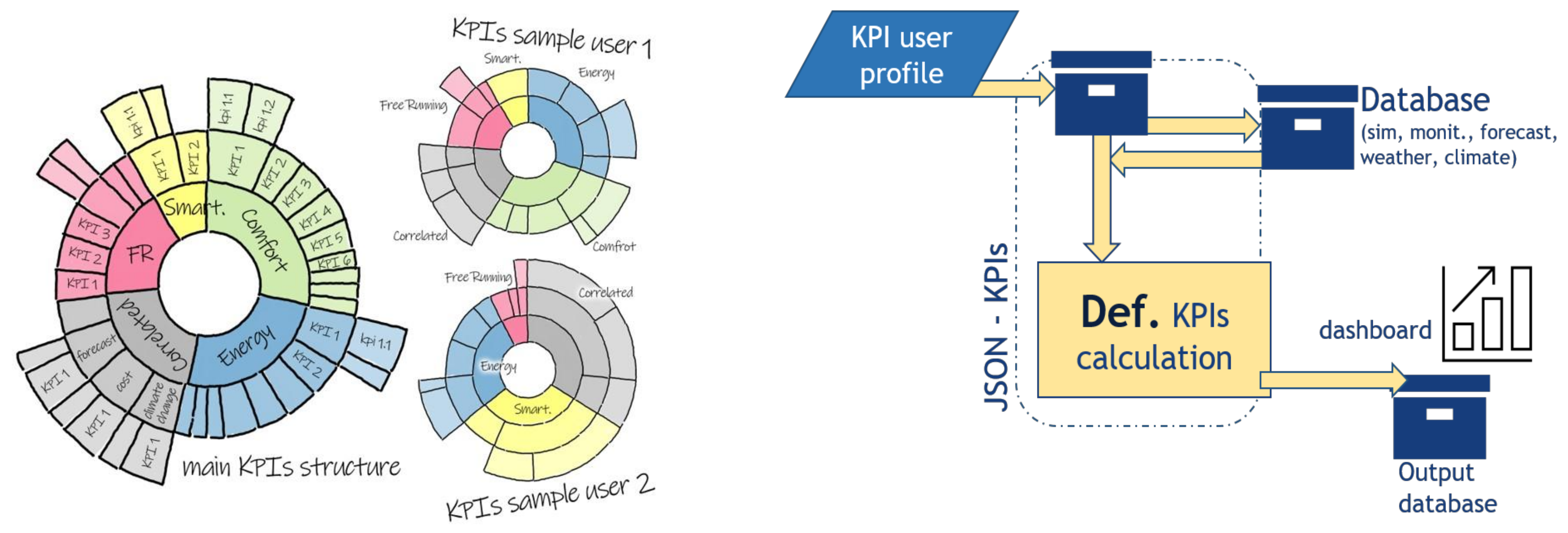
The proposed tool also includes graphical output analyses and the possibility to compute a large list of key performance indicators (KPIs), and other ones are being considered. Despite EnergyPlus already providing the possibility to compute a very large set of KPIs according to both US and European norms, a structured way of applying the same KPI computation methodology to both simulated results and data from the field is not common in the literature. Additionally, the tool is conceived to support free-running usage for buildings (potential, exploitation, controlling actions), and other functionalities, such as including buildings without mechanical systems (especially cooling ones)—e.g., historical and traditional Mediterranean buildings—in a dynamic labelling approach. Moreover, the tool also works as a library so that expert users can exploit the already present classes and methods to create different sets of code with their own approaches and expand the potentialities of the tool.

Objectives and Structure

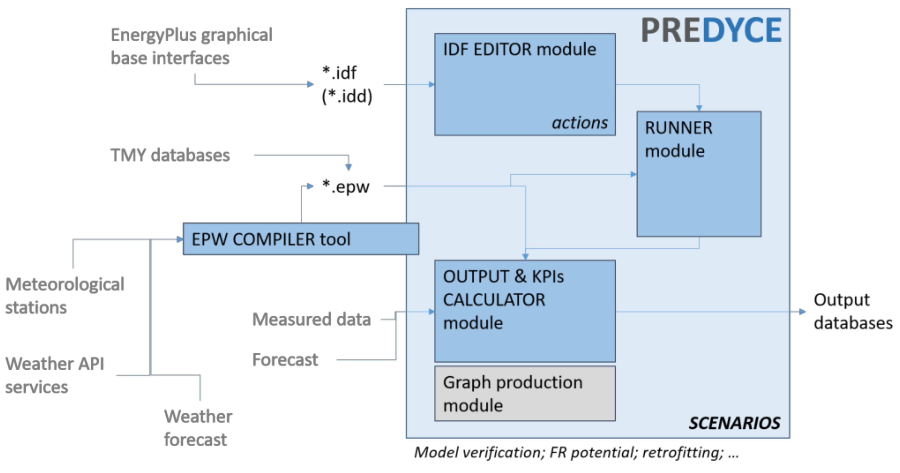
This paper introduces the initial architecture of a new Python-based tool which is able to script existing EnergyPlus input files, support sensitivity analysis, elaborate outputs and calculate KPIs (e.g., thermal comfort, indoor air quality, free-running potential, ventilative cooling), manage parallel simulation runs with an asynchronous multiprocessing approach and support the integration of extra modules. The tool, which is named PREDYCE (Python Realtime Energy DYnamics and Climate Evaluation), was/is being developed in two stages (development actions): (i) the “DYCE” action, and (ii) the “PRE” action.

In particular, the “DYCE” action included the definition of the initial tool structure, the development of a set of methods to modify EnergyPlus inputs according to a specific action list and the addition of calculation methods for KPIs connected to building design and post-operational data elaboration. Differently, the “PRE” action includes a set of extra scripting actions, including advanced functionalities—e.g., EnergyPlus-calculated natural ventilation, the possibility of scripting the simulation flow by integrating energy management system (EMS) objects to simulate control choices and running simulations on forecasted data to maximize free-running building potential; and developing user suggestions. In this second development action, more KPIs (e.g., climate correlated analyses and climate change resilience) and extra functions to support optimization actions (e.g., to maximize the exploitation of local free-running potential) will be added. The proposed tool also includes extra components to compile EnergyPlus weather files (*.epw) and functional actions to compare measured and simulated data. This paper focuses on the “DYCE” part of the tool, describing its main structure.

Hence, the paper’s main objectives are:

A.

To introduce the new tool, PREDYCE, supporting Python scripting for EnergyPlus runs and output elaborations focusing on the “DYCE” part of the tool.

B.

To show simple examples of use of “DYCE” functionalities of the tool, demonstrating the tool’s capabilities in typical use cases of parametric building analysis.

This last objective is composed of three more specific objectives:

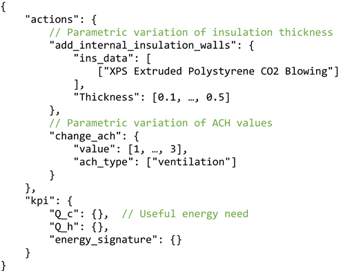
• To report an experiment involving a series of EnergyPlus input coding actions using a built-in JSON approach to test retrofitting functionalities (i.e., add insulation, change insulation thickness and substitute windows) on a mechanically heated and cooled sample building, and generating regression curves connecting variations in design inputs with changes in retrieved energy needs—early design steps.
• Report on a series of simulations of the same building with the same typical meteorological data (TMY) but focusing on free-running during the summer season alone. For this, simulations were performed in a second climate as well, to analyze results in a hotter area. During this test, automatic output elaboration was performed to calculate adaptive thermal comfort KPIs and to represent results using intuitive graphical outputs generated via the Python tool—early design steps.
• Report on a series of simulations of one of the E-DYCE demo buildings that involved automatically feeding EnergyPlus with measured weather data and automatically comparing simulation results with monitored data retrieved by sensors—operational steps.

These three specific objectives allowed us to test the initial version of the proposed tool for basic “DYCE” functionalities considering a mechanical building scenario, a free-running summer building scenario and an simple operational scenario.

Considering the mentioned objectives, the paper is organized as follows: (i) An overview of existing state-of-the-art tools able to modify EnergyPlus input files and/or to support manual or automatic parametric simulations—see Section 1. (ii) A materials and methods section introducing the general architecture of the tool and detailing the initial “DYCE” modules and functionalities—see Section 2.1 (Ob. A). (iii) Descriptions of the three testing scenarios, including adopted actions and parameter variations—see Section 2.2 (Ob. B). (iv) A section reporting and discussing the mentioned examples of use, including limitations, focalized on the outputs of the scenarios—see Section 3 (Ob. B.a, B.b and B.c). (v) A section devoted to conclusions and future development phases—see Section 4.

2. Materials and Methods

Section 2 is subdivided into two parts according to the two identified main objectives of the paper: Section 2.1 (Ob. A) and Section 2.2 (Ob. B).

2.1. Initial Architectural Scheme of PREDYCE

PREDYCE is a Python package with different modules which can be imported from other scripts in order to perform actions and analyses. A general scheme of the architecture is shown in Figure 1. The tool is based on three main modules—i.e., (i) the EnergyPlus input file (*.idf) editor, (ii) the KPI calculator and (iii) the runner module which is able to automatically manage multiple parallel simulations—along with extra modules supporting specific functionalities, e.g., to compile weather input files (*.epw) from different data sources. Moreover, input and database *.json files are used inside the tool to both define actions and KPIs to be performed and calculated, respectively, during a pool of simulations; and to store information necessary to modify *.idf files (e.g., compositions of materials, schedules and construction elements) in a dictionary form.

The integration of the described modules allows for a high level of automation in parametric building analyses, minimizing the user’s manual effort and not requiring or knowledge of Python. Additionally, the proposed tool being able to run on both personal computers and servers allows for massive simulations.

Table 1. Workflow of a generic PREDYCE application.

Not automated actions	(1) Create a base building model for EnergyPlus (*.idf file). (2) Compile an input *.json file, listing desired actions and ranges to be applied parametrically to the building model (e.g., Listing 1). (3) Script launch from command line, specifying as parameters at least the building model, the weather file and the input *.json file.
Automated actions	(4) Create a structured table listing all combinations of building parameters to be modified: each line will correspond to a specific building simulation and each column to building characteristics (e.g., insulation thickness, ventilation ACH, type of window system, …). (5) Asynchronous parallel launch of N simulations (automatically chosen by the code according to CPU characteristics or defined by the user). The N rows of the previously built table allow for the creation of N different *.idf files with the chosen characteristics. After each simulation KPIs are computed and building specific graphs produced. Numeric results are appended in new table columns and graphs saved in rows dependent folders. (6) Creation of a *.csv file containing aggregated and lightweight results for all simulations performed.
Not automated actions	(7) Analysis and plots generation from aggregated results.

summarizes the steps of a generic application workflow, highlighting the automated and still not automated processes. Particularly, steps (2) and (3) have the potential to be further simplified through the development of a simple GUI to launch simulations and choose among the list of pre-built actions. This is true thanks to the easy to compile *.json input file, which could future automatically created in future. Regarding step (3), the EnergyPlus command line launch structure made of options and an input *.idf file was kept (e.g., -w option is followed by the *.epw weather file) for users already used to EnergyPlus software. Furthermore, step (7) could be integrated into the automated process through the development of a post-process graph production module.

Algorithm 1. Example of an input *.json file to feed PREDYCE.

In the following, the functionalities of the tool’s main module are briefly described. The *.idf editor module is able to read, edit and save EnergyPlus input files. Such files are handled thanks to EPPy [9] scripting language. The complexity of the editing actions exclusively depends on how the different elements of the file are interconnected and interpreted by EnergyPlus during a simulation run; for this reason, manual editing of the input file could be very complex. The editor module instead offers a way to perform some such complex actions by means of Python methods that are easily callable from a custom script, simplifying the editing procedure. For example, when looking at Algorithm 1 it is possible to identify the add_internal_insulation_wall action that automatically modifies the base *.idf by adding a new layer in external walls (in this case in the innermost layer) composed by the mentioned material (selected from a *.json database internal to the tool) and whose thickness is varied in a given range by producing a large set of modified *.idf files.

The KPI calculator module is able to perform calculations and analyses, and graph plots by accessing EnergyPlus output files. Such actions can be automatically performed after each simulation, called by the runner module or manually executed by a custom Python script. The analyses usually consist of resampling output data and applying formulas to compute indicators based on European standards. Some calculations can also include graphs that can be saved in a subfolder structure in order to be associated with single simulations and visualized when needed. In the common case in which KPI methods are called by the runner module, all results are aggregated together in a final *.csv file in which each row represents a simulation and each column an output (including EnergyPlus base outputs if needed) or a computed KPI. KPIs are organized according to a modular approach—see Figure 2—considering five main domains (energy and energy efficiency; free-running operation and exploitation; comfort/quality; smartness, readiness and end-users; correlated indicators) and an implementable list of specific indices. The current version is available at [20]. This module was conceived to treat not only EnergyPlus outputs, but also data retrieved by monitoring campaigns or simulated by other tools to calculate and potentially compare relevant KPIs in multiple datasets. Hence, the module may treat simulated and monitored data about both buildings and climate issues. The specific KPIs adopted in this paper are described in Section 2.2 and are calculated via the code from the KPI module.

The runner module is a script including a Python class that can be instantiated and used by a user or by other tool modules to perform multiple simulations and analyses at once. The runner is in charge of creating a pool of simulations which are then executed in an asynchronous way by multiple instances of EnergyPlus on the same machine; this pool of simulations can be a simple combination of all possible actions described in the input *.json file by the user. Each simulation is executed on a building which has been modified by one or more actions from the input file. After each simulation phase, all KPIs are calculated and appended in the final output file. In the end, a final data frame of all simulated buildings is saved on a *.csv file in order to be further analyzed.

2.2. Test Scenarios (Examples of Use)

As mentioned before, three scenarios have been considered to initial test the proposed tool.

• Scenario A (Ob. B.a)—Mechanical building testing scenario.

Scenario A simulated a demo building implementing mechanical heating and cooling systems (simple HVAC) to calculate net energy needs and compute energy signatures in different retrofit cases. The base building model was parametrically modified by adding external insulation to the boundary walls and ceiling insulation in selected zones in a defined thickness range (range 2.5–30 cm, step 2.5 cm). Additionally, two types of window systems were tried (double glazing, clear, Low-E, with argon; and triple glazing, clear, Low-E, with air).

KPIs adopted in Scenario A were net energy needs and energy signature calculated in line with EN 15603:2008 [21]. The energy signature, 1D (based on external temperature) or 2D (external temperature and global horizontal solar irradiation), is a well-known indicator reported in several studies for different purposes, including comparisons of retrofitting scenarios—see, for example, ref. [22,23].

• Scenario B (Ob. B.b)—Summer testing scenario without mechanical cooling.

Scenario B simulated the demo building for the sole summer period (assumed from 1st of June to the 30th of September) without any cooling systems. The building was set to work in a free-running mode supporting ventilative cooling strategies—see the definitions of ventilative cooling reported in [24,25]. Different free-running modes were compared by parametrically changing ventilation ACHs (with values 0, 2.5 and 5), the length of a shading overhang (range 0.2–1 m, step 0.2 m) and the external shade rolls’ control strategy based on outdoor dry bulb temperature (range 20–30 °C, step 2 °C) and horizontal global solar irradiation (range 100–500 W/m², step 50 W/m²) thresholds. The shading control strategy was not differentiated based on zone or orientation, but was applied to all windows.

With the demo building being located in a cold climate area—Torre Pellice municipality, northwest of Italy, in a mountain valley—the summer discomfort expected was limited, so the same building was simulated also in a hotter climate (Rome) to demonstrate the tool’s potential for supporting free-running indicators and suggesting correlated early design choices.

The KPIs adopted in Scenario B are related to building free-running mode. In particular, distribution of datapoints in adaptive comfort model categories was calculated assuming the adaptive thermal comfort model of EN 16798-1:2019 [26]. Additionally, the percentage outside the range (POR) was calculated—see Equation (1).

$$POR=\frac{{{\displaystyle \sum }}_{i=1}^{Oh}wf ·h_i}{{{\displaystyle \sum }}_{i=1}^{Oh}{h}_i \left[0-1\right]}$$

(1)

POR returns the percentage of cumulated occupied hours ($Oh$) when thermal comfort is not reached (weighting factor discomfort hours $wf=1$, comfort hours $wf=0$) with respect to total occupied hours in the calculation period—see, for example, ref. [11]—assuming as the thermal comfort boundary a predicted mean vote (PMV) value (Fanger thermal comfort model, i.e., ISO 7730 [27]) or an operative temperature threshold in an adaptive comfort model. Considering the residential usage of the demo and the COVID pandemic, the calculations were performed for this paper for the whole period rather than typical occupancy hours. Considering the PMV-PPD model, boundaries of comfort category III were assumed, i.e., $\mathrm{abs}\left(PMV\right)=0.7$, which corresponds to a predicted percentage of dissatisfied (PPD) of 15% [26]. For the latter model, a metabolic rate of 1.2 met was assumed [28] as the average for domestic spaces, and clothing values were set, respectively, to 1 clo and 0.5 clo for Torre Pellice (mountain site) and Rome. Considering instead an adaptive comfort model, ACM discomfort was defined as the percentage of hours outside category II boundaries. The proposed tool also already integrates additional indicators, e.g., climate correlated indices of the location, including degree-days/degree-hours, ventilative cooling and other low-energy technology indices—see IEA EBC Annex 62 [24,29].

• Scenario C (Ob. B.c)—Operational testing scenario (simulation and measured data).

Scenario C focused on operational analyses. The same demo building was, for this scenario, simulated with measured weather data. Simulation results were compared with measured environmental conditions for the same period, June 2021, taking into account internal air temperatures $T_{db}^i$. Considering the building’s specific usage, average values of main zones were used for analyzing simulation results and real data. The proposed tool is able to support real-time or post-analyses by comparing simulated data with measured data to analyze the free-running potential and its exploitation, and to support decision making. Additionally, calibration supporting actions were performed to include the possibility of implementing the model verification method described in [30] and advanced methodologies for more automatic procedures. The original model was compared with the verified model after the application of the calibration signature methodology mentioned before—see also Equation (2)—exploiting the massive simulation potential of the proposed tool.

$$\mathrm{Calibration} \mathrm{signature}=\frac{\mathit{measured} T_{db}^i-\mathit{simulated} T_{db}^i}{\mathit{max}\mathit{measured} T_{db}^i}\cdot 100\%$$

(2)

The optimization procedure was meant to reduce the combined error measure defined by Equation (3) and was based on parametric changes in the U-value for both walls and roofs, changes in the windows’ thermal characteristics (U-value and SHGC), changes in internal mass, changes in equipment’s internal gains and changes in ACH for both ventilation and infiltration.

$${\mathrm{Error}}_{\mathrm{tot}}=\sqrt{RMS{E}^2+MB{E}^2}$$

(3)

where RMSE and MBE are, respectively, the well-known statistical indices root mean square error and mean bias error.

In particular, by selecting each time a subset of parameters to be varied in specified ranges (e.g., −30% to +30% of base model values), a pool of simulations was created from which the building variant which gave the lowest error was taken as a local minimum. This step was executed at first on the building envelope; then on ACH; and finally, on the other parameters until all of them were tested (around 600 simulations in total) in order to find an optimized subset for all parameters, despite not leading to a global minimum. In line with the mentioned reference, different parameters may be assumed according to the specific type of building and the inspection plan followed (e.g., if verified dimensions of windows are missing, their area may be included in variations).

The Simulated Demo Building

An existing residential building was selected for the tests. The building is representative of typical Italian houses located in small municipalities. The specific building is located in Torre Pellice (northwest of Italy), a small municipality in a mountain valley, and is monitored as a demo case in an on-going project [31]. The access to monitoring data allowed us to perform Scenario C. This real building was chosen to show the ability of the tool to support simulations even of models derived from real buildings, which are expected to be more specific and complex with respect to typical simplified buildings. This demo building is composed by a single flat adjacent to unoccupied and not heated/cooled spaces above (roof) and below (storage). Furthermore, the flat’s boundary walls are unattached to any other structure, with the exclusion of a 39 m² that is adjacent to another flat, which was simulated by assuming the same thermal characteristics. Finally, part of the floor is directly adjacent to the ground (48 m² over 118 m² of total conditioned floor area, including the unoccupied technical space which is also conditioned). The walls are composed of stone and aggregates with internal and external plaster (traditional building) with an average thickness of 50 cm. The stone roof is divided into a cold part (unconditioned space in Figure 3) composed by a stone layer without insulation; an area adjacent to the conditioned zone is defined by an uninsulated slab; and a warm part that was recently retrofitted, including 10 cm of thermal insulation and an internal finish with matchboard. The building was first modelled using DesignBuilder v6 to develop a base *.idf file—see the 3D schematic model in Figure 3—and secondly, this initial model was used as the initial input file to feed the simulation tool.

Schedules, reference parameters and setpoints for energy calculations were retrieved by default values suggested in EN 16798-1:2019 [26], Annex C, considering the residential apartment user profile; occupancies were adapted according to specific zone types adopting from the suggested DesignBuilder profiles. When mechanical systems were considered (e.g., Scenario A), setpoints during occupied hours were set to 20 °C (winter) and 26 °C (summer), considering thermal comfort category II of ISO 7730 and EN 16798-1. A setback of 18 °C was considered for the heating system during unoccupied hours. For the purpose of mentioned testing scenarios, equipment was auto-sized by EnergyPlus, considering ideal loads. Humidity is not controlled in this house, in line with typical Italian residential systems (heating is performed by radiators, and cooling is absent or rarely driven by sensible split units). Free-running analyses were performed only for the cooling period; this choice is consistent with traditional Italian houses that generally have a heating system but do not have a cooling system. For free-running simulations, the building was simulated without a cooling system, considering the sole summer period from the 1st of June till the 30th of September. Scenario A was simulated under Torre Pellice’s climate conditions. For Scenario B both Torre Pellice and a hotter location were selected. The latter was the Casaccia site, near Rome, Italy, which was selected in order to test summer free-running KPIs in a location with higher cooling needs, even if for the purpose of this paper all simulations were performed using the same building. Both typical weather files were generated by Meteonorm [32].

Considering Scenario C, the mentioned demo building was equipped with monitoring sensors able to collect environmental (and energy) data and to transmit them via SOAP [33]. In particular, all rooms of this residential unit are monitored using the Capetti Winecap system [34]. Air temperature is collected in all rooms, and main rooms are also checked for relative humidity. The kitchen/living room also has a CO₂ sensor. All data are collected every 10 min. Specific code was developed to collect data via API requests, filter them and define average hourly values. Considering the specific usage of the building—i.e., the doors between main rooms are always open—both monitored and simulated data (for living, kitchen–living room and bedroom) were averaged before comparisons. Weather data were retrieved by means of a REST API by the E-DYCE meteorological station installed on a near demo building (distance: 815 m).

3. Examples of Use and Discussion

This section describes and discusses the three mentioned testing scenarios.

3.1. Scenario A

For Scenario A, the proposed tool was used to run a sensitivity analysis, allowing us to compare the impacts of different retrofitting choices regarding energy needs for the specific building under a Torre Pellice TMY. About 500 simulations were run for this purpose, thereby automatically generating 500 different *.idf files which differ from the base one not only in the changes of thickness values but also by the presence of new material layers which have impacts on geometry. A unique output *.csv file containing aggregated results was then used to perform classic post-analysis comparisons. 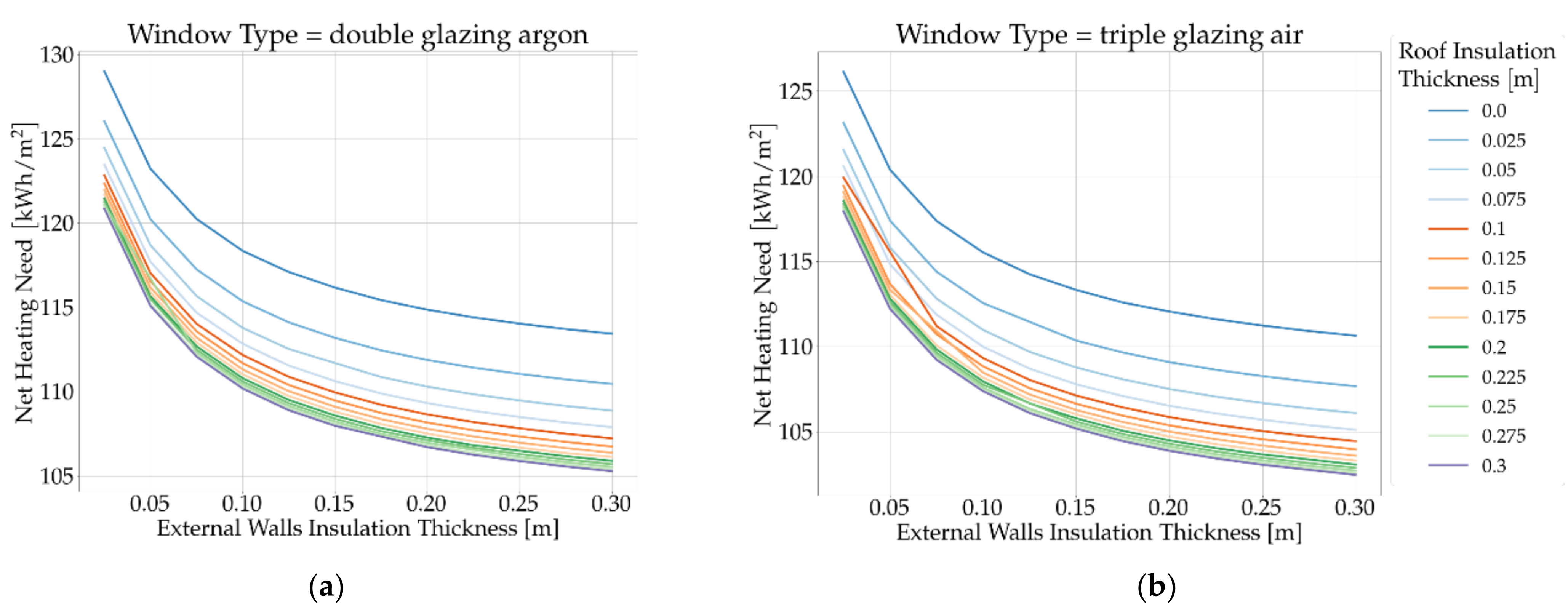Figure 4 shows correlations between wall insulation thickness and annual energy needs for different roof insulation levels. When increasing the boundary walls’ insulation thickness, a reduction in energy needs occurred, and as expected, the first 10–15 cm of insulation had the greatest impact. More roof insulation allows for extra reductions in energy needs. Similarly, Figure 4b analyses the impacts of wall and roof insulation thicknesses when windows are triple glazed. In the latter case, a slight reduction in net energy needs is clear due to lower U-value of triple-glazed windows.

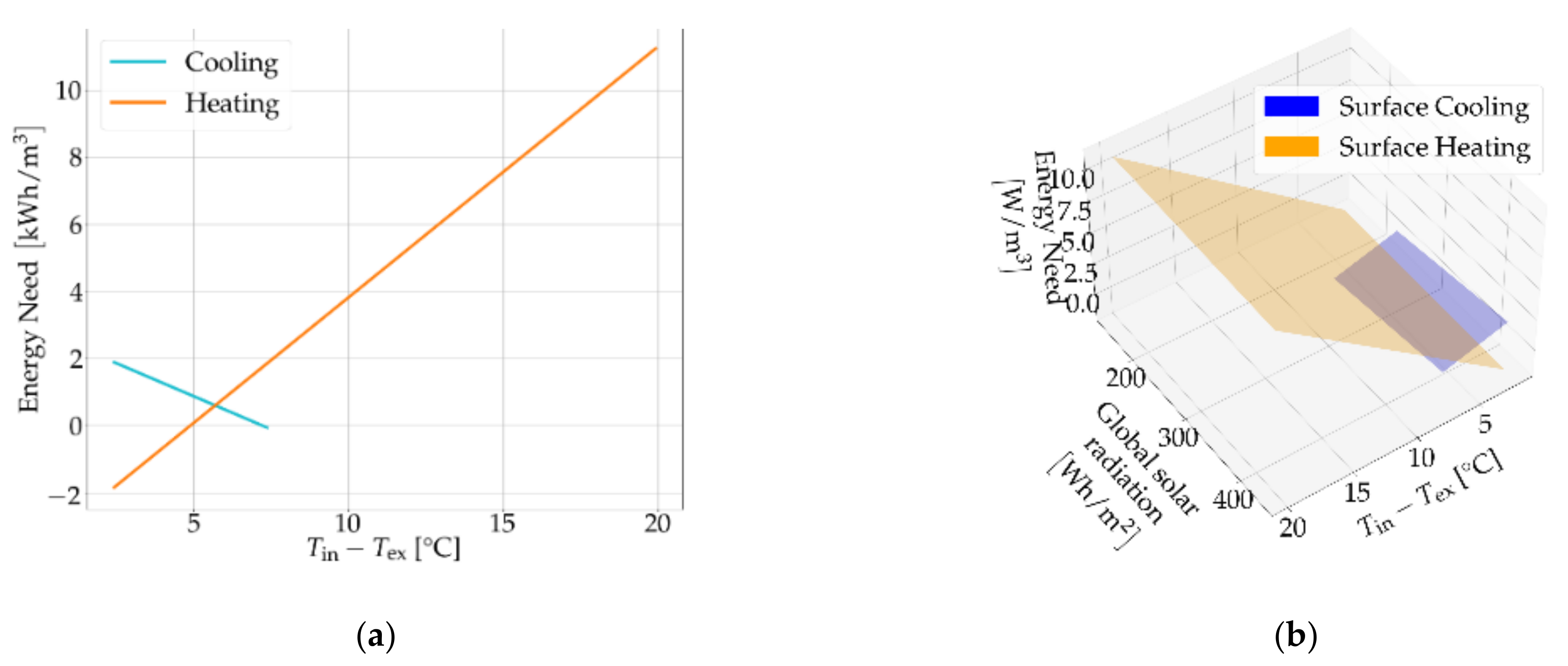
Figure 5 shows 1D and 2D energy signatures for the best case in terms of net energy needs. For the considered case, the impact of weekly averaged global solar irradiation (not considering the nights) was very low with respect to outdoor temperature; similar results were retrieved in other studies in cold climates [35]. Additionally, since the demo case is located in a mountainous area, the cooling system’s contribution to the net annual energy needs is not relevant. As mentioned above, the KPI module allows one to calculate KPIs with simulated data or other data, including monitored data. Focusing on the energy signature, this KPI supports data-driven building-energy-use models that account for the influences of outdoor conditions on heat consumption, to allow fast heating responses—see, for example, studies on data-driven model definitions [36,37]—but also will allow comparing design-driven signatures with monitored ones.

3.2. Scenario B

In the summer free-running mode scenario, the impacts of different technologies were analyzed on the demo building in both a cold (Torre Pellice) and a hot (Casaccia) Italian climate, resulting in about 1600 simulations. The weather file was used as a parameter in the specific parametric set adopted for this example.

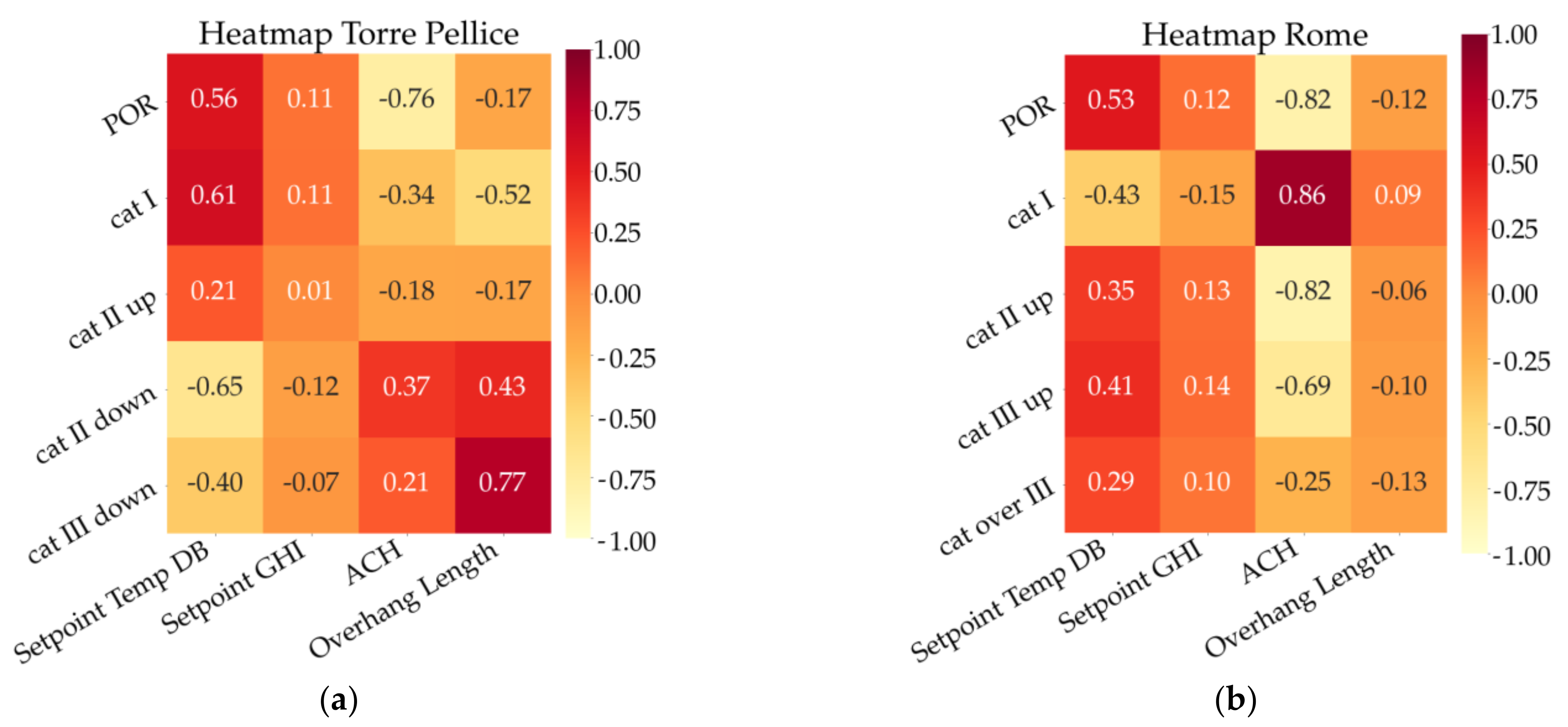
Figure 6, for example, shows the linear impacts the adopted free-running technologies have on thermal comfort. In the colder Torre Pellice climate, the reduction of the overhang length in order to increase direct solar gains had a strong impact on reducing the number of hours in adaptive comfort category II or III, considering the bottom boundaries causing a shift to upper categories. I.e., for Torre Pellice, overhang length had the highest impact on category III (0.77), decreasing discomfort (too cold). In parallel, raising the outdoor temperature threshold (so almost never activating the shading) also led to a benefit. Instead, in the hotter Rome climate, increasing the ventilation and reducing the outdoor temperature threshold provided thermal comfort benefits in terms of point distribution in adaptive comfort model categories. For example, the increase in airflow supported a growth in hours in the comfort category I (+0.86) and a reduction in hours above a suitable temperature in categories II (−0.82), III (−0.69) and III (−0.25). This type of statistical heatmap analyses allows one to study correlations between design aspects and KPIs, while considering single and combined technologies, helping designers to find optimal early design choices or to understand the impacts that a choice may have on the building. The proposed tool performs this design support action thanks to the automatic generation and running of multiple massive simulations.

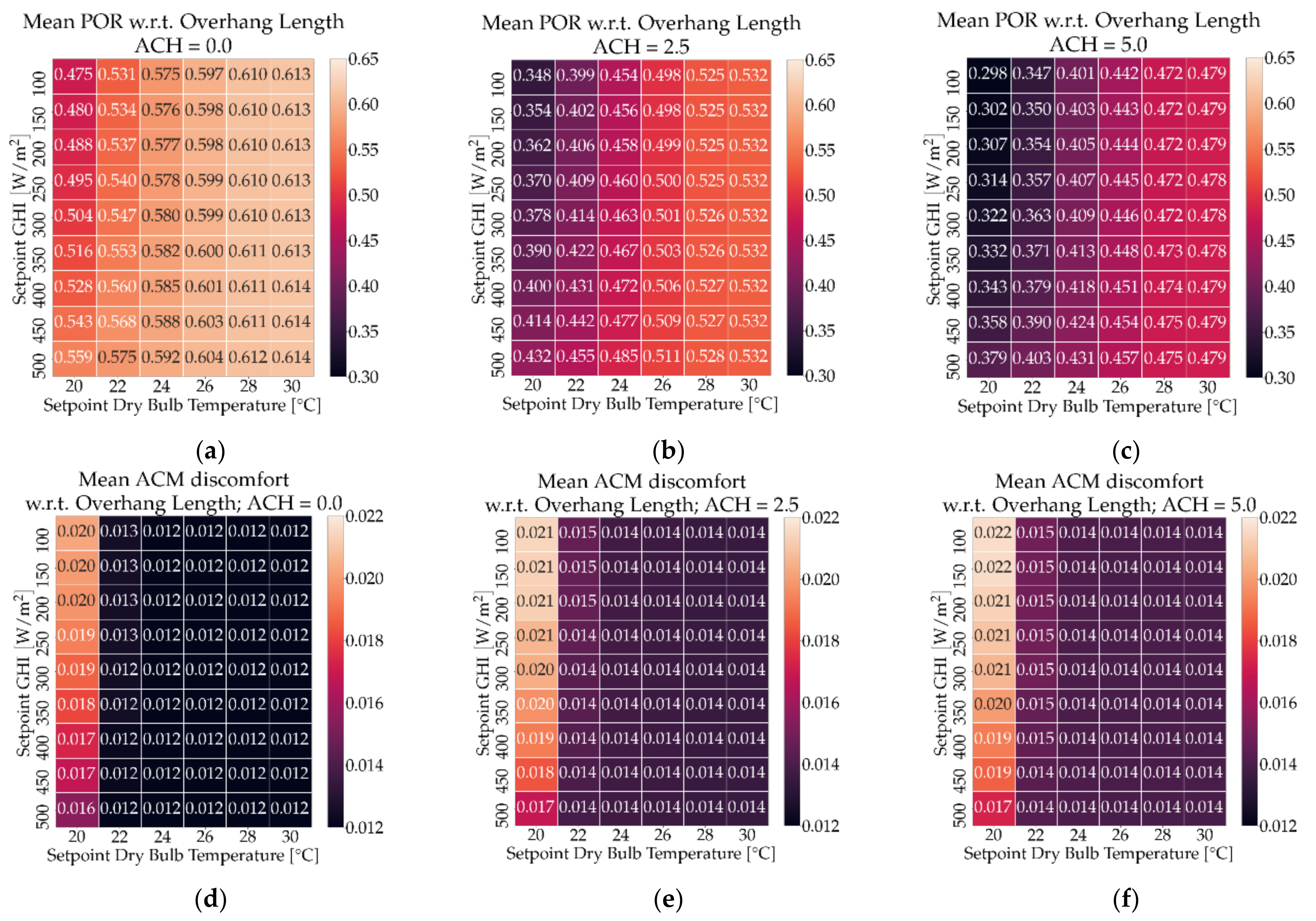
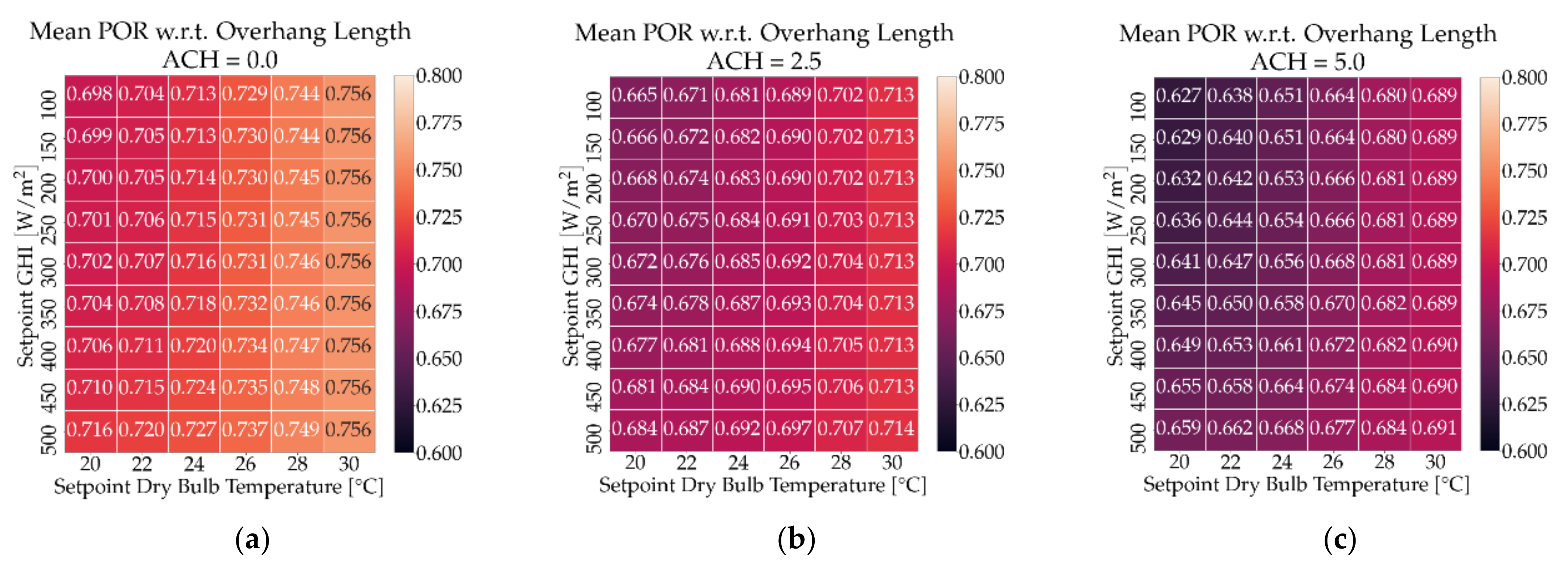
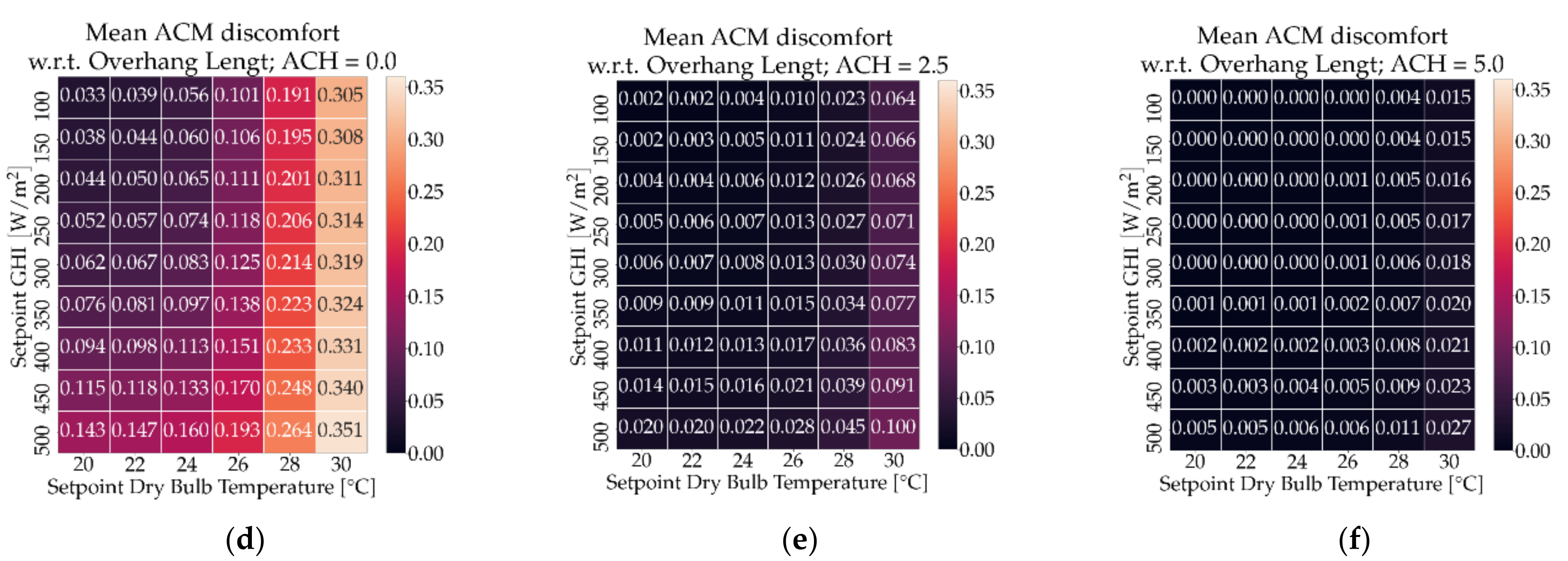
Figure 7 and Figure 8 show in greater detail the impact of the roller shades’ activation strategy on thermal discomfort. We varied ACH and averaged on results obtained with different overhang lengths. For this test, scheduled natural ventilation was assumed in order to support early design analyses for the climate potential of ventilative cooling; nevertheless, the proposed tool also allows one to include calculated natural ventilation when needed. ACH variations support, in early design stages, different control strategies using openings for natural ventilation, which can be further detailed in advanced design stages—see [38]—but may also represent the airflows to be contributed by a detached mechanical ventilation system. Considering Torre Pellice, Figure 7 shows that ACM discomfort and POR (based on PMV) have opposite behaviors. This suggests, as expected, that the PMV-PPD model is more sensitive to uncomfortable hot perception, possibly accentuated by having the value closet to 1, despite the shift of hours from lower to higher adaptive comfort model categories. For Rome, Figure 8, the two indicators show the same behavior, being positively impacted by low solar irradiation and temperature thresholds.

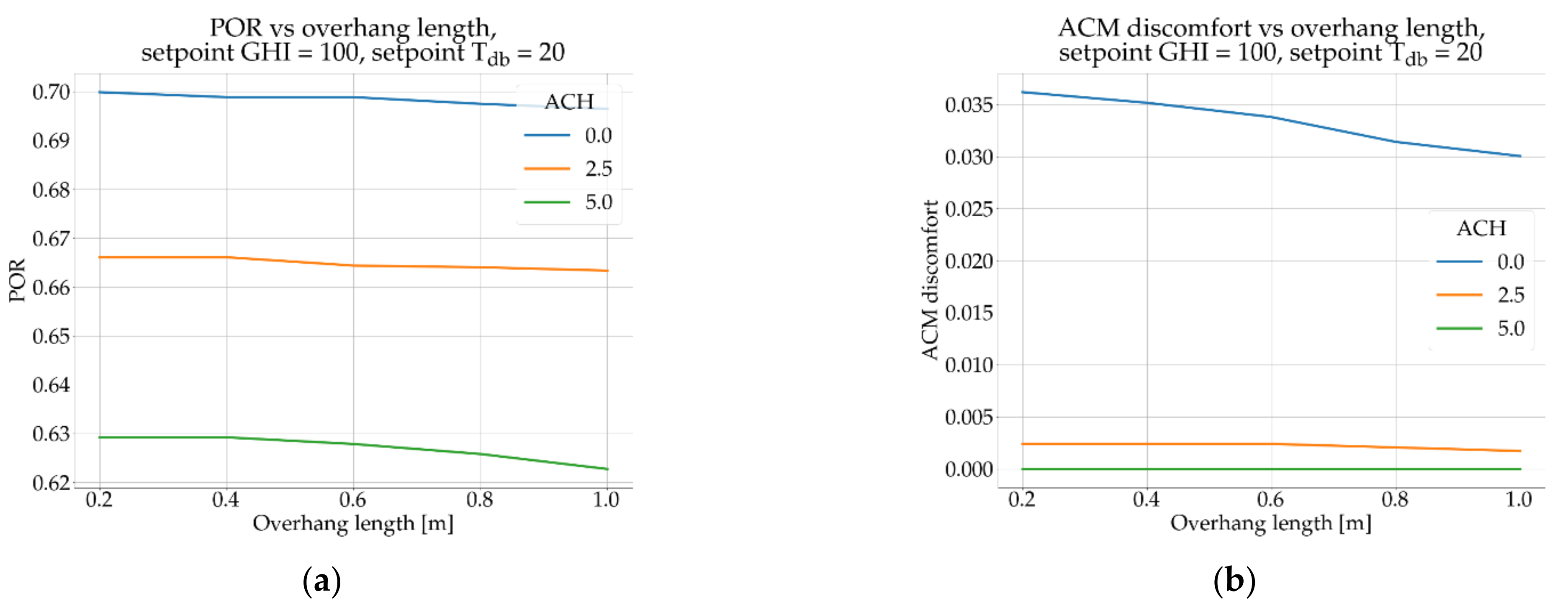
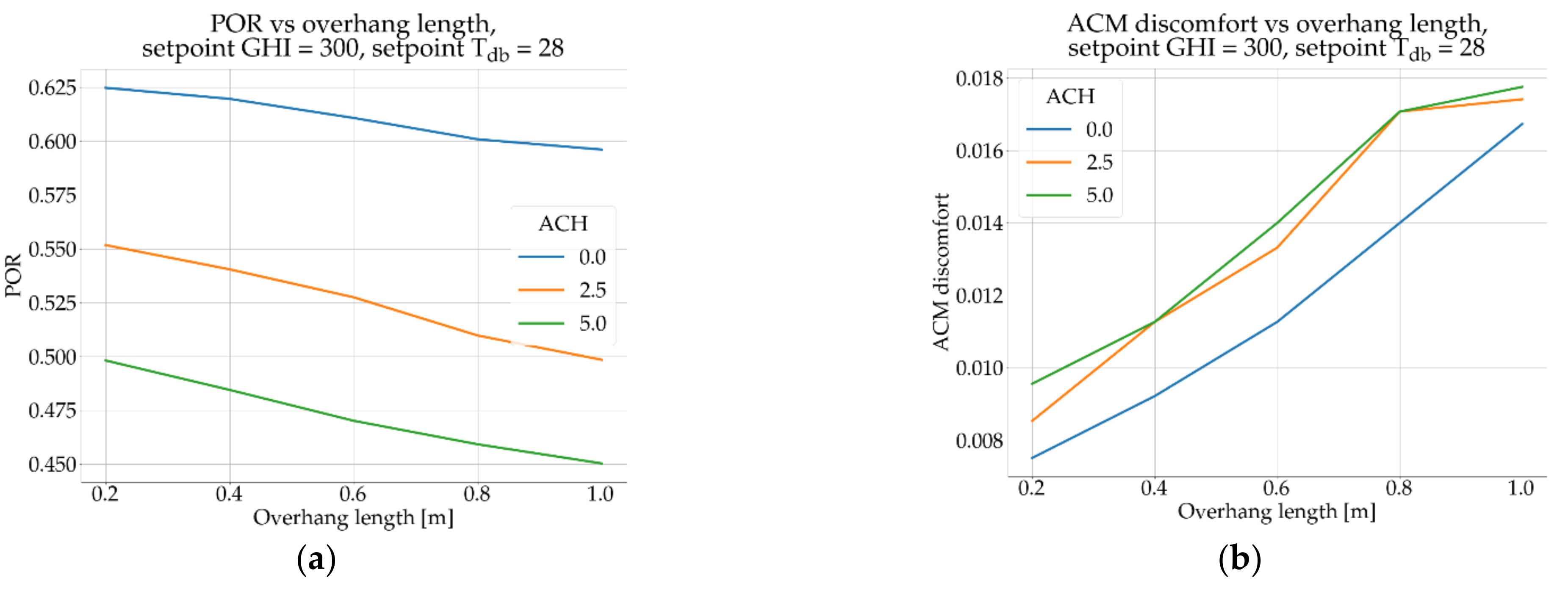
Figure 9 and Figure 10 show the impact of overhang length on thermal discomfort, considering optimized values of shading control thresholds. The opposite behaviors of POR and ACM discomfort were again evident for the case of Torre Pellice. In Rome, with higher ACH values, the impact of overhang was less relevant, causing a slight increase in discomfort even.

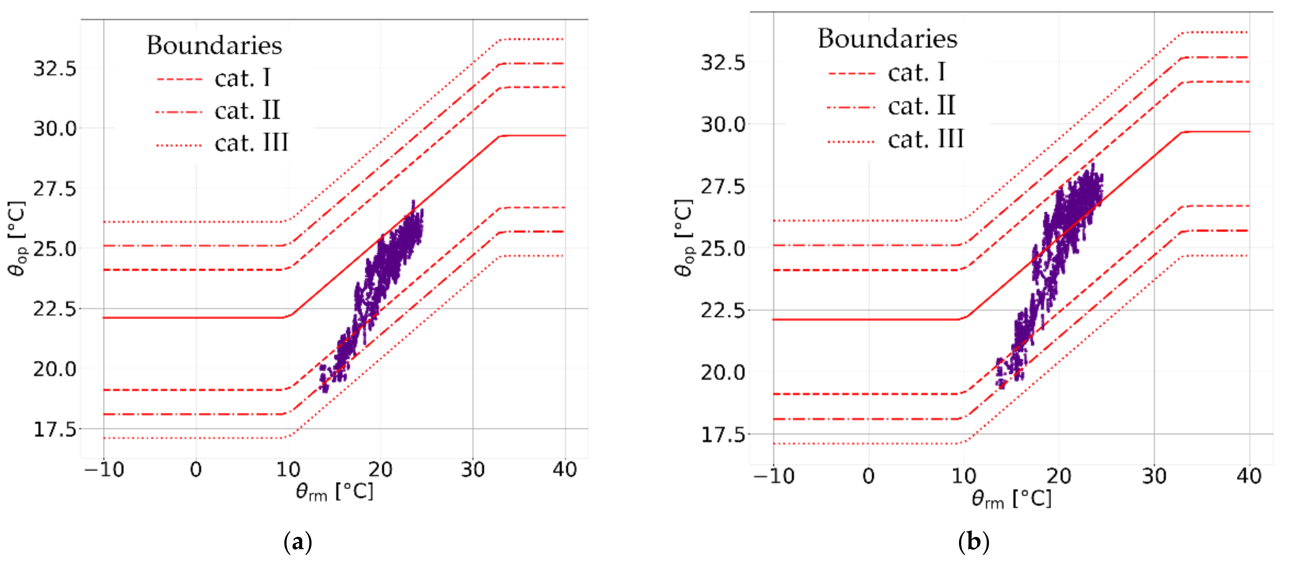
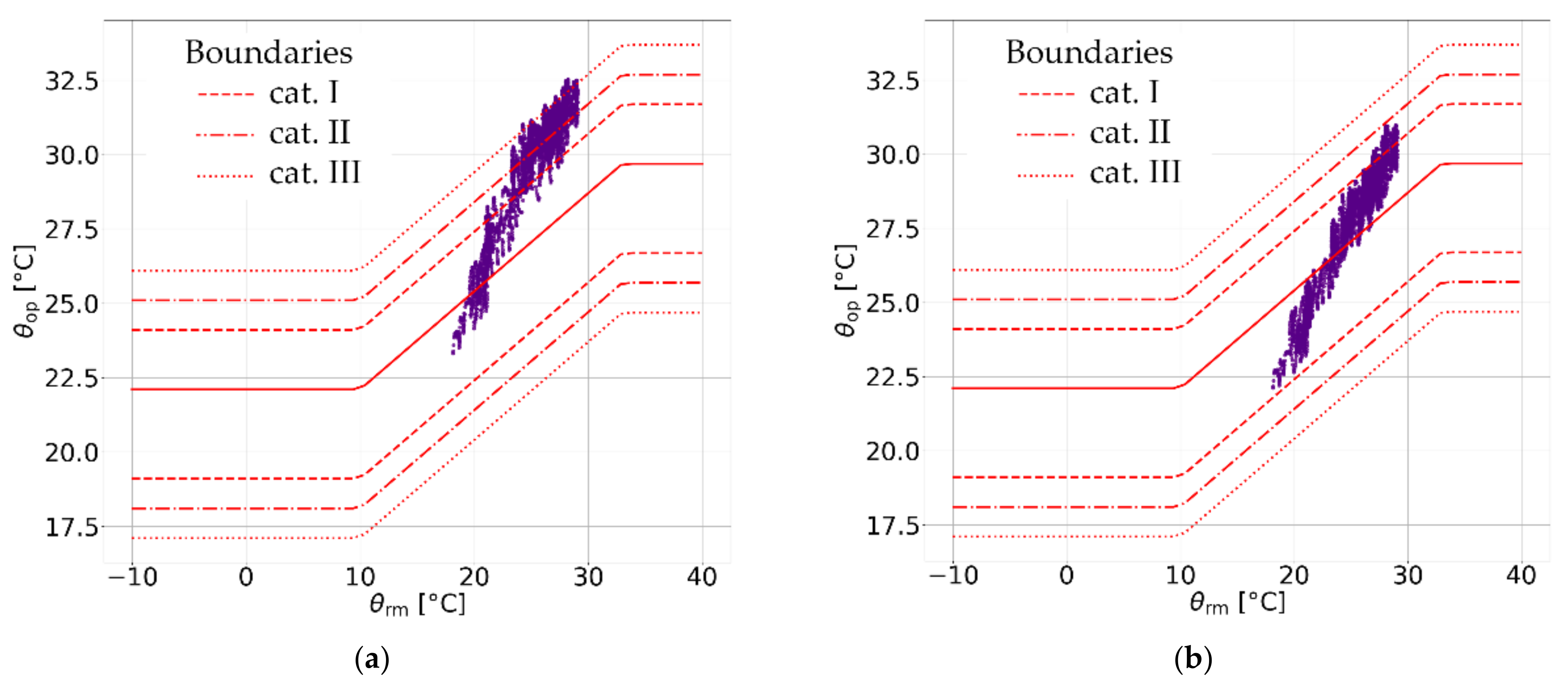
Figure 11 shows how an optimized combination of free-running technologies allowed us to slightly warm up the house in summer in the mountainous area, and Figure 12 shows the more interesting opposite behavior in a hotter climate, where optimized strategies allowed us to maintain indoor operative temperatures almost entirely inside adaptive comfort model category II without the need for a mechanical cooling system.

3.3. Scenario C

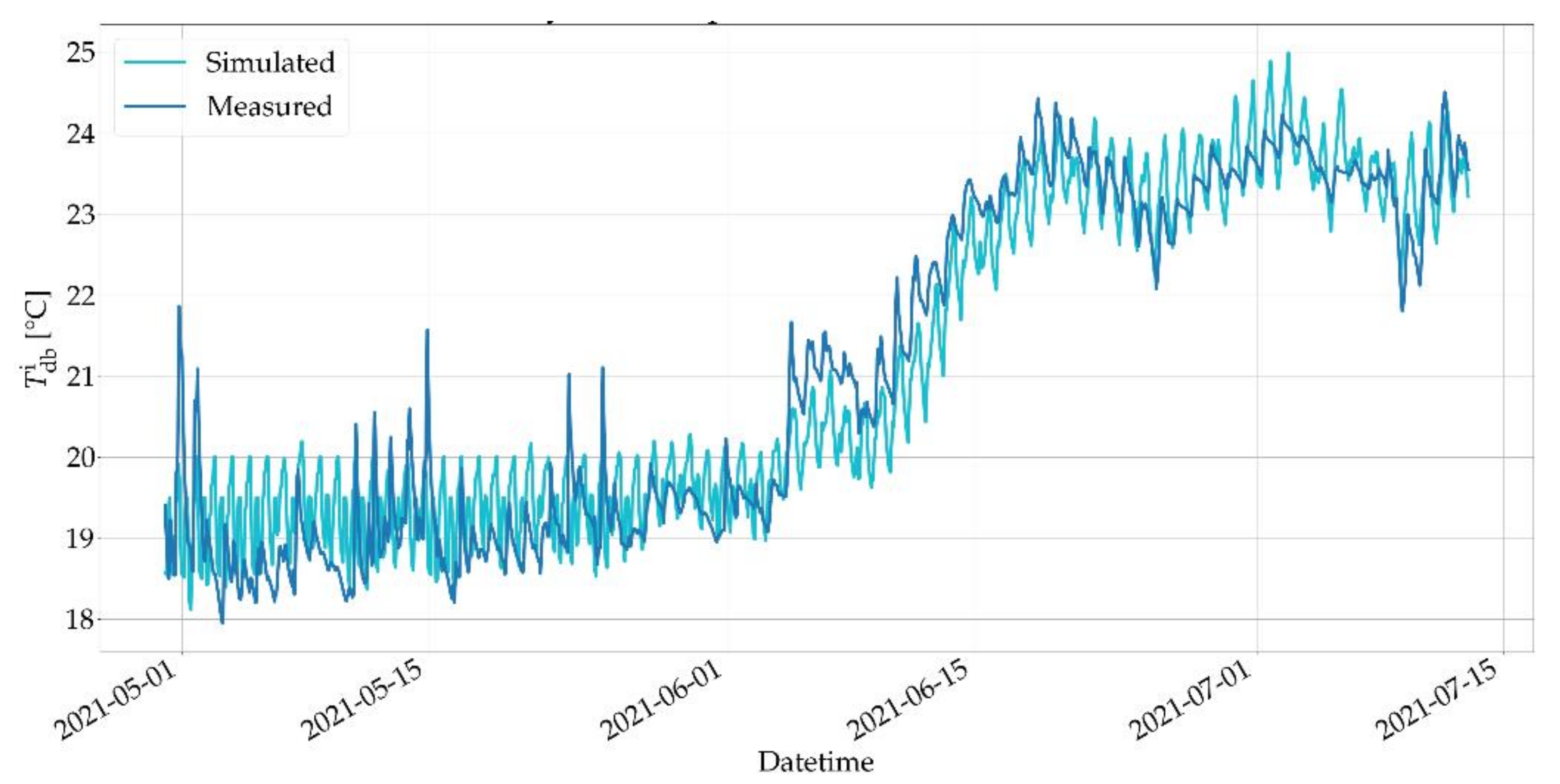
Figure 13 shows the simulated base model and the monitored indoor air temperatures, considering the same period of time and the same monitored weather data: the errors on the model correspond to a RMSE equal to 0.670 and an MBE equal to 0.342 for indoor air temperature. A semi-automatic verification process was performed to adjust the building model to fit data measured in June 2021—see the description in Section 2.2. 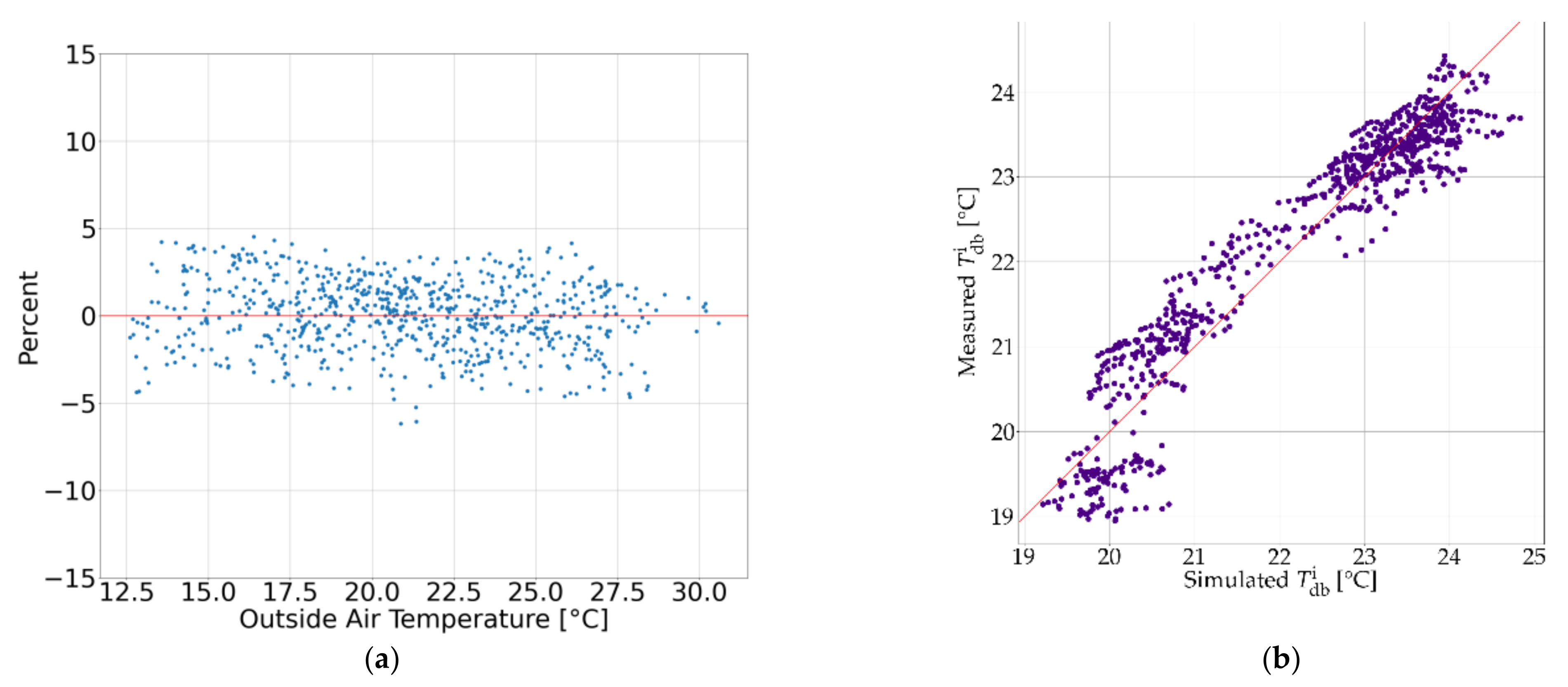Optimized values of RMSE equal to 0.486 and MBE equal to −0.02 were then obtained, and Figure 14a shows the calibration signature for the best case.

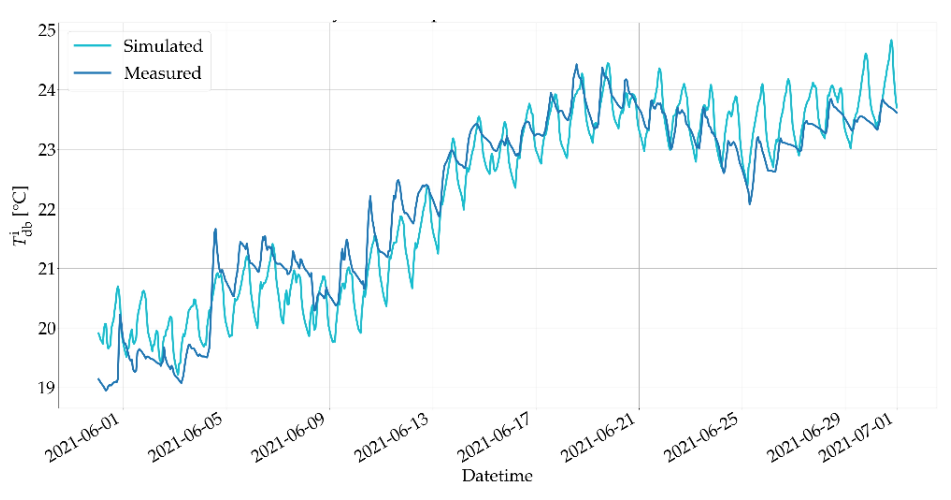
Figure 14b shows the distribution of measured indoor temperatures versus simulated ones in the best case: higher temperatures were better verified, whereas middle and lower ones clearly shifted, even if the calibration signature errors did not exceed 5%. Further optimization is expected during the next implementation phases of the verification part of the code. Figure 15 instead shows optimized simulated and measured indoor temperatures over the period of time considered in the verification process. At the end of the month, it is possible to identify some days in which the simulated and monitored error gets larger, especially during hourly peaks, but it is known that those days correspond to a vacation period for the tenant, resulting in lower thermal gains in the monitored data (simulation occupancy and gains are not changed).

3.4. Discussion and Limitations

The auto-generated pool of simulations and the automatic result aggregation approach of the proposed tool allow one to easily run large sensitivity analyses that include modifications to several building and control system parameters.

At present, uses such as model verification or retrofitting require simple but detailed setups by a user, who must manually select tasks, parameters and actions to be performed in order to achieve the desired workflow and final results compiled in an input *.json file. Nevertheless, alongside the possibility of selecting specific features or combinations of features and KPIs, future usage scenarios are expected to be developed. A usage scenario is a pre-defined set of changes in the *.idf input and output KPIs that can be identified by users by a sole name (e.g., retrofit) instead of mentioning all actions (change insulation thickness, change window, etc.).

Regarding the performance, the time it took to run 500 annual simulations (including model editing, post-processing and KPI calculations) of Scenario A on a modern desktop PC (AMD Ryzen™ 7 2700X Processor) was about 5 h; 1600 summer simulations of Scenario B on a high-end server (AMD EPYC™ 7662 Processor) took about 30 min; Scenario C, which consisted of the multi-step model verification task, took about 10 min on the same server as well. For a better understanding of such benchmarks, it has to be considered that manually performing small building editing could take up to three minutes; executing every simulation one by one and comparing the results to find the best case could take up to 6 h with 150 simulations. Similarly, if we consider performing the same 150 simulations by manually changing inputs, running simulations, collecting and analyzing results, e.g., in excel, about 50 h is to be expected (20 min each). The approach offered by the proposed tool, of automatically creating and running all different buildings given the initial instructions, can reduce the working time to 20 min when using a modern high-end laptop (11th Generation Intel^® Core™ i7 Processor) or even to 2 min when using a dedicated server (AMD EPYC™ 7662 Processor).

The adoption of more advanced optimization algorithms in order to reduce the number of simulations to reach the optimum will be implemented in the near future. Finally, the development of an extra functionality to pass from net to primary and source energy consumptions considering dynamic COP (coefficient of performance) is expected, in line with hourly EU standards for energy performance certification (EPC).

4. Conclusions

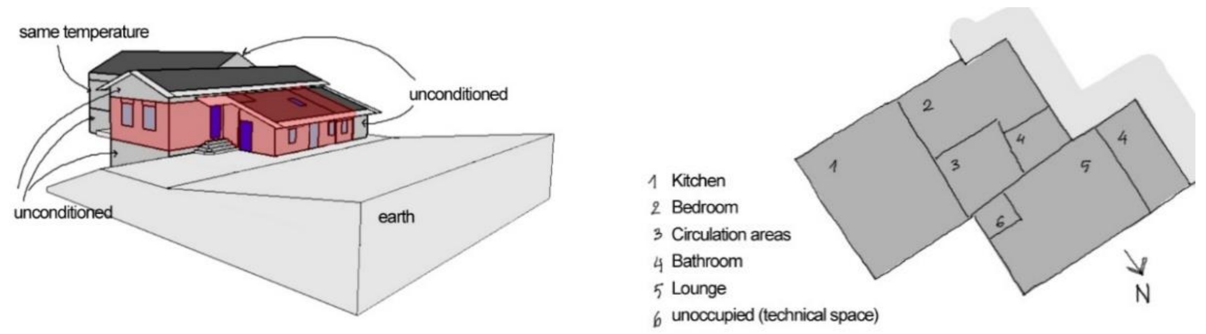
This paper introduced a new Python-based tool able to edit EnergyPlus inputs, manage a large set of simulations and support KPI calculations for different purposes and usage scenarios. The new tool, PREDYCE, was briefly described, and the initial functionalities were tested on a demo case of the EU H2020 project E-DYCE, which was represented by a single residential unit in a terraced house. The tool is based on three main modules: an input editor, a runner and a KPI calculator. Extra modules are under development, e.g., to support measured data actions. We intend for this tool to be used with not only user-built lists of inputs and outputs, but also to simulate pre-built scenarios (e.g., model verification, sensitivity analyses, operational suggestions and free-running potential), based on pre-created input *.json files that may be recalled via a future graphical interface. These potentialities will be the core of the following months’ expansions.

Moreover, this paper reported the outputs of the first successful simulations (testing scenarios). Scenario A demonstrated that the proposed tool includes actions able to support early design retrofit analysis, and that it may calculate simple energy performance indicators in a graphical form. Scenario B showed the potentialities of the tool for supporting free-running mode optimization, especially for summer, including some devoted KPIs and analyses. Scenario C demonstrated the potentialities of integrating both weather and environmental monitoring data for model verification and operative purposes in the data analysis pipeline. Currently, the proposed tool allows one to compare different retrofitting scenarios by building simulations to identify energy optima; nevertheless, a comprehensive approach including economic analyses is under development to align the development of the retrofitting scenario with global cost (EN 15459-1:2017 [39]) and the cost optimal vision—see, for example, the approach in [40,41].

The main functionalities of the tool are in place, and during the next two years, it will be further tested in applications on a large set of demo cases based in Europe, and it will be used to support and test design methodologies and suggestions. These testing and application phases are expected to support the definition of additional actions and KPIs; the development of an API launching interface so remote users and third party servers can control the tool; the definitions of simple action combinations in scenarios; and the inclusion of extra functionalities, i.e., supporting prescient building optimizations and analyzing free-running potential exploitations. Two application development lines will be focused on: the first—supporting design choices and optimization; and the other—supporting operational choices and control evaluations. Additionally, extra functionalities, such as climate change impacts on the geo-climatic applicability of low-energy technologies, will be added in the “PRE” developing action [42].

References

1. DOE; NREL. EnergyPlus™; DOE: Washington, DC, USA; BTO: Tokyo, Japan; NREL: Golden, CO, USA, 2020. [Google Scholar]
2. SCI; TRANSSOLAR; CSTB; TESS. TRNSYS—Transient System Simulation Tool; TESS: Madison, WI, USA, 2019. [Google Scholar]
3. University of Illinois. LBNL EnergyPlus Documentation-External Interface(s) Application Guide; Guide for Using EnergyPlus with External Interface(s); University of Illinois: Urbana, IL, USA, 2015. [Google Scholar]
4. IBPSA EnergyPlus Graphical Interfaces 2021. Available online: http://www.buildingenergysoftwaretools.com/?capabilities=Whole-building+Energy+Simulation&keywords=EnergyPlus (accessed on 28 September 2021).
5. NREL; ANL; LBNL; ORNL; PNNL. OpenStudio. 2021. Available online: https://www.openstudio.net/ (accessed on 28 September 2021).
6. DesignBuilder Software. DesignBuilder; DesignBuilder Software: Gloucestershire, UK, 2020. [Google Scholar]
7. Building Energy Modeling with Openstudio: A Practical Guide for Students and Professionals; Springer Science+Business Media: New York, NY, USA, 2018; ISBN 978-3-319-77808-2.
8. jE+ JEPlus—An Parametric Tool for EnergyPlus and TRNSYS 2019. Available online: http://www.jeplus.org/wiki/doku.php?id=start (accessed on 28 September 2021).
9. Santosh, P. Eppy. 2021. Available online: https://pypi.org/project/eppy/ (accessed on 28 September 2021).
10. Energy in Cities Group; University of Victoria. BESOS—Building and Energy Systems Optimization and Surrogate-Modelling. 2020. Available online: https://besos.uvic.ca/ (accessed on 28 September 2021).
11. Guo, R.; Hu, Y.; Liu, M.; Heiselberg, P. Influence of Design Parameters on the Night Ventilation Performance in Office Buildings Based on Sensitivity Analysis. Sustain. Cities Soc. 2019, 50, 101661. [Google Scholar] [CrossRef]
12. Gordillo, G.C.; Ruiz, G.R.; Stauffer, Y.; Dasen, S.; Bandera, C.F. EplusLauncher: An API to Perform Complex EnergyPlus Simulations in MATLAB® and C#. Sustainability 2020, 12, 672. [Google Scholar] [CrossRef] [Green Version]
13. Huberman, N. Energy Efficient Strctural Form: Analysis and Applications for Desert and Seismic Areas. Ph.D. Thesis, Ben-Gurion University of the Negev, Beer-Sheva, Israel, 2012. [Google Scholar]
14. Chiesa, G.; Huberman, N.; Pearlmutter, D.; Grosso, M. Summer Discomfort Reduction by Direct Evaporative Cooling in Southern Mediterranean Areas. Energy Procedia 2017, 111, 588–598. [Google Scholar] [CrossRef]
15. Chiesa, G.; Grosso, M.; Acquaviva, A.; Makhlouf, B.; Tumiatti, A. Insulation, Building Mass and Airflows-Provisional and Multi-Variable Analysis. SMC|Sustain. Mediterr. Constr. 2018, 8, 36–40. [Google Scholar]
16. Chiesa, G.; Acquaviva, A.; Grosso, M.; Bottaccioli, L.; Floridia, M.; Pristeri, E.; Sanna, E. Parametric Optimization of Window-to-Wall Ratio for Passive Buildings Adopting A Scripting Methodology to Dynamic-Energy Simulation. Sustainability 2019, 11, 3078. [Google Scholar] [CrossRef] [Green Version]
17. Faure, G.; Christiaanse, T.; Evins, R.; Baasch, G.M. BESOS: A Collaborative Building and Energy Simulation Platform. In Proceedings of the 6th ACM International Conference on Systems for Energy-Efficient Buildings, Cities, and Transportation, New York, NY, USA, 13 November 2019; ACM: New York, NY, USA, 2019; pp. 350–351. [Google Scholar]
18. Baasch, G.; Westermann, P.; Evins, R. Identifying Whole-Building Heat Loss Coefficient from Heterogeneous Sensor Data: An Empirical Survey of Gray and Black Box Approaches. Energy Build. 2021, 241, 110889. [Google Scholar] [CrossRef]
19. Westermann, P.; Evins, R. Using Bayesian Deep Learning Approaches for Uncertainty-Aware Building Energy Surrogate Models. Energy AI 2021, 3, 100039. [Google Scholar] [CrossRef]
20. EDYCE. D1.2 Operational Dynamic Energy Perfomance Certificate (EPC) Specifications; PoliTO: Turin, Italy, 2021; p. 159. Available online: https://edyce.eu/wp-content/uploads/2021/01/E-DYCE_D1.2_Operational_dynamic_EPC_specifications_18.12.2020_Final.pdf (accessed on 28 September 2021).
21. EN 15603:2008. In Energy Performance of Buildings. Overall Energy Use and Definition of Energy Ratings; CEN: Brussels, Belgium, 2008; ISBN 978-0-580-59028-3.
22. Ghiaus, C. Experimental Estimation of Building Energy Performance by Robust Regression. Energy Build. 2006, 38, 582–587. [Google Scholar] [CrossRef]
23. Pasichnyi, O.; Wallin, J.; Kordas, O. Data-Driven Building Archetypes for Urban Building Energy Modelling. Energy 2019, 181, 360–377. [Google Scholar] [CrossRef]
24. Chiesa, G.; Heiselberg, P.K.; Kolokotroni, M. Innovations in Ventilative Cooling; Springer International Publishing: Cham, Switzerland, 2021; ISBN 978-3-030-72384-2. [Google Scholar]
25. Heiselberg, P. IEA EBC Annex 62—Ventilative Cooling Design Guide; Aalborg University: Aalborg, Denmark, 2018; p. 122. [Google Scholar]
26. European Committee for Standardization. EN 16798-1:2019—Energy Performance of Buildings—Part 1: Indoor Environmental Input Parameters for Design and Assessment of Energy Performance of Buildings Addressing Indoor Air Quality, Thermal Environment, Lighting and Acoustics; European Committee for Standardization: Brussels, Belgium, 2019. [Google Scholar]
27. EN ISO 7730:2005. In Ergonomics of the Thermal Environment. Analytical Determination and Interpretation of Thermal Comfort Using Calculation of the PMV and PPD Indices and Local Thermal Comfort Criteria; CEN: Brussels, Belgium, 2006; ISBN 0-580-47207-8.
28. Nicol, F.; Humphreys, M.A.; Roaf, S. Adaptive Thermal Comfort: Principles and Practice; Routledge: London, UK; New York, NY, USA, 2012; ISBN 978-0-415-69159-8. [Google Scholar]
29. Kolokotroni, M.; Heiselberg, P. IEA EBC Annex 62—Ventilative Cooling State-of-the-Art Review; Aalborg University: Aalborg, Denmark, 2015. [Google Scholar]
30. Claridge, D.; Paulus, M. Building simulation of practical operational optimisation. In Building performance simulation for Design and Operation; Hensen, J., Lamberts, R., Eds.; Routledge: London, UK; New York, NY, USA, 2019; pp. 399–453. ISBN 978113839219. [Google Scholar]
31. CORDIS Energy Flexible DYnamic Building CErtification 2020. Project Information. Available online: https://cordis.europa.eu/project/id/893945 (accessed on 28 September 2021).
32. Meteotest. Meteonorm; METEOTEST Genossenschaft: Bern, Switzerland, 2015. [Google Scholar]
33. Snell, J.; Tidwell, D.; Kulchenko, P. Programming Web Services with SOAP, 1st ed.; O’Reilly & Associates: Sebastopol, CA, USA, 2002; ISBN 978-0-596-00095-0. [Google Scholar]
34. Capetti Elettronica Capetti Winecap System 2021. Available online: http://www.capetti.it/index.php/winecap (accessed on 28 September 2021).
35. Nordström, G. Use of Energy-Signature Method to Estimate Energy Performance in Single-Family Buildings; Open WorldCat: Luleå, 2014; ISBN 978-91-7583-023-0. [Google Scholar]
36. Ascione, F.; Bianco, N.; De Stasio, C.; Mauro, G.M.; Vanoli, G.P. Simulation-Based Model Predictive Control by the Multi-Objective Optimization of Building Energy Performance and Thermal Comfort. Energy Build. 2016, 111, 131–144. [Google Scholar] [CrossRef]
37. Cholewa, T.; Siuta-Olcha, A.; Smolarz, A.; Muryjas, P.; Wolszczak, P.; Anasiewicz, R.; Balaras, C.A. A Simple Building Energy Model in Form of an Equivalent Outdoor Temperature. Energy Build. 2021, 236, 110766. [Google Scholar] [CrossRef]
38. Grosso, M. Il Raffrescamento Passivo Degli Edifici, 4th ed.; Maggioli: Sant’Arcangelo di Romagna, Italy, 2017; ISBN 8891622204. [Google Scholar]
39. EN 15459:2007. In Energy Performance of Buildings. Economic Evaluation Procedure for Energy Systems in Buildings; CEN: Brussels, Belgium, 2007; ISBN 978-0-580-56482-6.
40. Fregonara, E.; Verso, V.R.M.L.; Lisa, M.; Callegari, G. Retrofit Scenarios and Economic Sustainability. A Case-Study in the Italian Context. Energy Procedia 2017, 111, 245–255. [Google Scholar] [CrossRef] [Green Version]
41. Chiesa, G.; Fregonara, E. Energy and Economic Analyses for Supporting Early Design Stages: Introducing Uncertainty in Simulations. In Sustainability in Energy and Buildings; Littlewood, J., Howlett, R.J., Capozzoli, A., Jain, L.C., Eds.; Smart Innovation, Systems and Technologies; Springer: Singapore, 2020; Volume 163, pp. 49–60. ISBN 978-981-329-867-5. [Google Scholar]
42. CORDIS Prescient Building Operation Utilizing Real Time Data for Energy Dynamic Optimization 2020. Project Information. Available online: https://cordis.europa.eu/project/id/958345 (accessed on 28 September 2021).
Figure 1. Draft of the PREDYCE architecture. Note: *.idf is a file with idf extension.
Energies 14 06429 g001
Figure 2. (a) The adopted modular approach to KPIs [20] and (b) the PREDYCE organization of the output and the KPI calculator module.
Energies 14 06429 g002
Figure 3. The initial model of the demo building developed using an EnergyPlus graphical interface.
Energies 14 06429 g003
Figure 4. Retrieved simulation results plotting net energy needed for different wall and roof insulation thicknesses—that is, substituting current windows (a) with a double gazing with argon, or (b) triple glazing with air.
Energies 14 06429 g004
Figure 5. 1D (a) and 2D (b) energy signatures with weekly data aggregation for best case in terms of total annual energy needs (ceiling insulation 30 cm, external wall insulation 30 cm and triple glazed windows).
Energies 14 06429 g005
Figure 6. Heatmaps showing correlations of free-running technologies and simulated thermal comfort/discomfort in Torre Pellice (a) and Rome (b) climates.
Energies 14 06429 g006
Figure 7. Simulated POR (ac) and adaptive comfort model discomfort (df) in Torre Pellice. Outdoor temperature and global solar irradiation thresholds vary for activation of shade rolls.
Energies 14 06429 g007
Figure 8. Simulated POR (ac) and adaptive comfort model discomfort (df) in Rome. Outdoor temperature and global solar irradiation thresholds vary for activation of shade rolls.
Energies 14 06429 g008aEnergies 14 06429 g008b
Figure 9. Thermal discomfort expressed with (a) POR and (b) adaptive categories at varying overhang length and ACH in Torre Pellice.
Energies 14 06429 g009
Figure 10. Thermal discomfort expressed with (a) POR and (b) adaptive categories at varying overhang length and ACH in Rome.
Energies 14 06429 g010
Figure 11. Distribution of datapoints in adaptive comfort categories for (a) worst and (b) best free-running summer modes in Torre Pellice. Dashed and dotted lines represent adaptive comfort categories’ boundaries.
Energies 14 06429 g011
Figure 12. Distribution of datapoints in adaptive comfort categories for (a) worst and (b) best free-running summer modes in Rome. Dashed and dotted lines represent adaptive comfort categories’ boundaries.
Energies 14 06429 g012
Figure 13. Indoor air temperatures simulated and measured over the period of time, considering base building model (not optimized).
Energies 14 06429 g013
Figure 14. Calibration signature (a) and temperatures (b) of optimized building model.
Energies 14 06429 g014
Figure 15. Indoor air temperatures simulated and measured over the considered verification time period, with optimized building parameters.
Energies 14 06429 g015