On the Use of Base Temperature by Heat Cost Allocation in Buildings

Abstract

Heat cost allocators (HCAs) have a high market share in existing buildings, which may cause problems, especially with variable heat cost allocation due to wrong readings from HCAs and/or the method used in the heat cost allocation process. That is why we proposed two easily applicable and clear methods, which may be used with two types of HCAs commonly used in the billing practice. The proposed methods were presented on the example of the actual allocation of variable heating costs for a multi-family building located in Poland, and the results of billing were compared with three other methods of variable heating costs allocation. Owing to the proposed methods, higher (K = 0.5260 for schema A, K = 0.4468 for schema B) values of the correlation coefficient between heating costs and the average indoor temperature were obtained than for the methods commonly used in accounting practice. Additionally, the use of the proposed method allows for the elimination of defective indications of heat cost allocators in the billing process and discrepancies in the indications of HCAs in individual flats, which do not have technical justification and violate the norms of social coexistence.

1. Introduction

The obligation of individual accounting of heating costs in multi-apartment buildings with a central heat source was introduced under the Directive [1].

On the one hand, this allowed for the reduction of heat consumption for heating in existing buildings [2,3,4,5], owing to a more rational behaviour of users of the apartments equipped with heat cost allocators (HCAs) or heat meters [6], but on the other hand, it contributed to the problems with heat costs allocation (especially variable costs) between individual flats in the building [7].

This is due to the fact that in individual countries, various methods and assumptions are used in individual accounting of heating costs, which are mainly based on the readings from HCAs or heat meters, which was presented in the review article [8].

For example, Pakanen and Karjalainen [9] and Siggelsten [10] proposed taking into account the heat transfer between apartments in the process of heat cost allocation.

In this aspect, Michnikowski [11] proposed the method of taking into account the heat transfers between the apartments by using average indoor temperature. Dell’Isola et al. [12] proposed a method for heat accounting in buildings, which takes into account the building inefficiencies and, thus, encourages the occupants to retrofit their flats. In another paper, Dell’Isola et al. [13] developed a model for creating reliable heat accounting systems in new buildings and estimating the reliability of heat accounting systems in existing buildings.

Aside from the well-known method of heat cost allocation (which makes use of HCAs or heat meters), Dell’Isola et al. [14] presented a tool that may increase user awareness of the existing problems by processing the basic data related to indoor air temperature and energy consumption in buildings. Saba et al. [15] proposed an indirect method for heat cost allocation, which takes into account the opening time of radiator valves, the heating medium temperature on supply and return, flow rate, indoor temperature and radiator characteristic coefficients. Canale et al. [16] estimated the influence of using in-home displays on the energy used for heating.

However, HCAs still have a very high market share in existing buildings and a simple method of heat cost allocation, which allows separation (using different types of HCAs) of the amount of heat from external sources (heating systems) from internal heat gains and heat gains from the sun, is lacking. Additionally, the proposed method should consider the issues related to indoor thermal comfort conditions in order to avoid extreme behaviour of occupants who may even lower the indoor air temperature below the acceptable value in order to achieve energy savings.

Therefore, this article proposed two methods that would allow for bridging this research gap and dividing the variable heating costs, with consideration of the heat supplied to given flats from external sources, using HCAs with the function of determining the indoor temperature in the flats (schema A) and HCAs without such a function (schema B). The proposed method also considered the level of indoor temperature in heated rooms by the heat cost allocation process, which may positively influence the indoor thermal comfort conditions.

The main goal of the article was to present a simple and user-friendly method of dividing variable heating costs using HCAs with the function of determining the indoor temperature in flats and HCAs without this function. An additional aim of the article was to present a comparison of the proposed methods of heat cost allocations with other methods that are commonly used in billing practice.

The second section presents the assumptions and principles of the proposed methods of variable heat cost allocation, while Section 3 presents the detailed accounting of variable heating costs using the proposed methods on the example of a multi-family building (see Section 3.2.1 and Section 3.2.2) and then comparing them with other methods of heat cost allocation (see Section 3.2.3).

2. Method

Developing a simple method of heat costs allocation that allows the amount of heat from external sources (heating systems) to be separated without internal heat gains and heat gains from solar radiation is a complex process. Therefore, the procedure for determining the base temperature is presented first (see Section 2.1), which was then used in the proposed method of heat costs allocation for the systems with HCAs, allowing for the determination of the average indoor temperature in the flats (see Section 2.2) or for a system with HCAs without such a function (see Section 2.3).

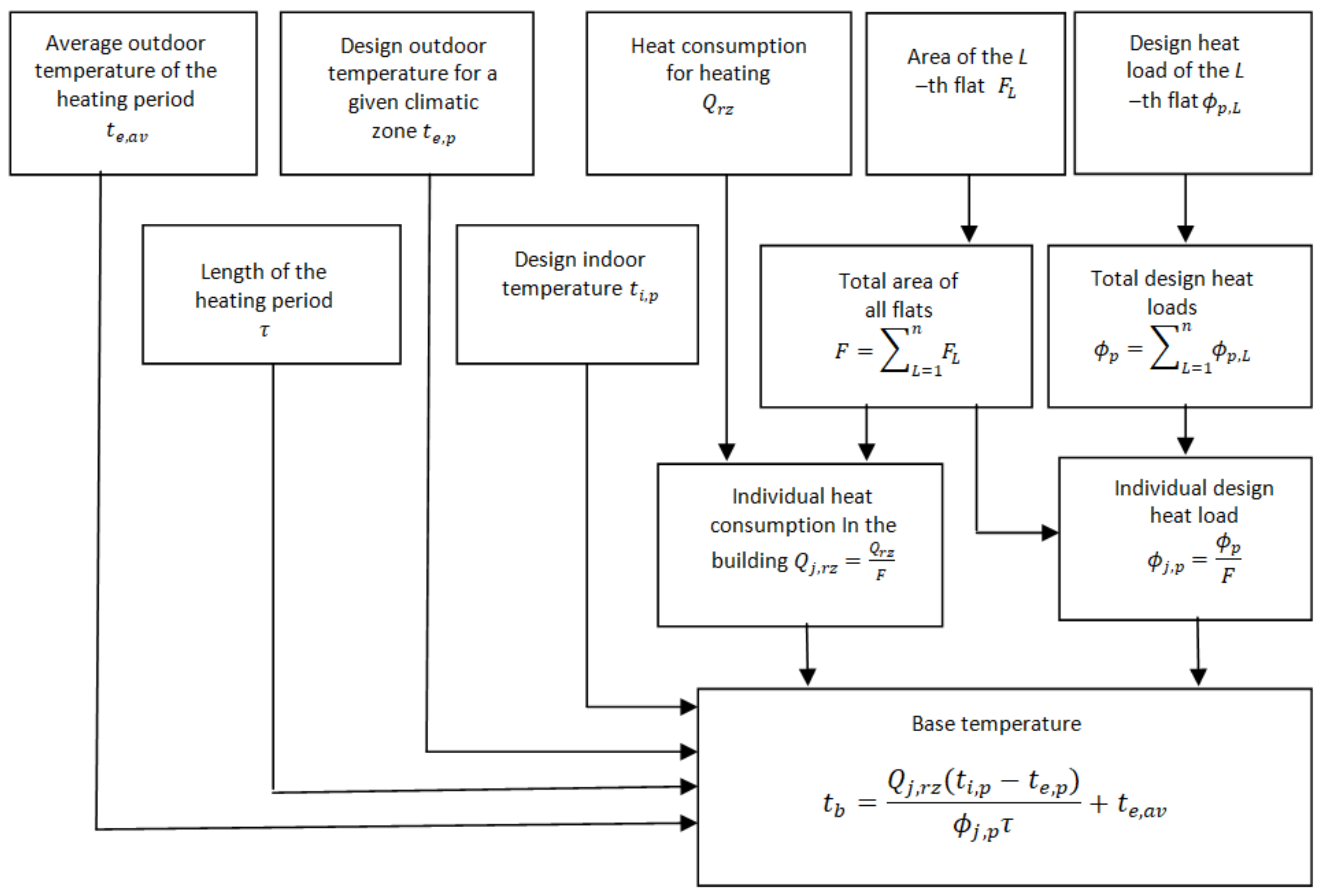
2.1. Estimation of Base Temperature for the Building

For the purposes of understanding the process of determining the base temperature (Figure 3), which can be used to determine the consumption of heat supplied to the flats by the heating system (external source), and then in the process of heat costs allocation, a detailed explanation of the assumptions and the calculation process are presented below.

Individual HCA indications in the building, i.e., the quotient of the sum of the normalized consumption units of HCAs and the sum of the areas of the settled flats, should be a function of its technical parameters as well as the length of the heating season, the average outdoor temperature in the heating season, and the average indoor temperature of all flats equipped with HCAs. Taking this into account, in any heating period in each accounting unit (building or group of buildings supplied from a single source), the individual heat consumption for heating can be assigned in physical units (e.g., GJ or kWh) or allocation units for a known average indoor temperature in the flats equipped with HCAs.

On the other hand, the knowledge about the dependence of the individual heat consumption, or the consumption units of HCAs on the average indoor temperature of all flats in the building, allows for the determination of the individual heat consumption for the average indoor temperature of any flat in the building.

Knowing that the heat supplied from external sources (in particular the heating system) and the heat from heat gains are used to heat the building to a given indoor temperature, then, in the case of an outdoor temperature higher than the base temperature characteristic for a given building, no heat supply (from external sources) for heating is required, as shown in Figure 1.

Thus, the base temperature (t_b), otherwise known as the temperature of the equilibrium point or the heating limit, is the value of the outdoor air temperature at which the instantaneous heat demand supplied by the central heating system to the building is zero, i.e., the heat losses through transmission and ventilation are fully covered by the generated heat gains from the sun, internal sources of heat, or heat gains from people.

Figure 1 shows a diagram of the dependence of the individual heat consumption for heating a building (Q_j) on the outdoor temperature (t_e). With the above-mentioned considerations in terms of t_b, the line parallel to the outdoor temperature axis (line A-B in Figure 1) divides the graph into two parts: (i) the upper part shows the dependence of heat consumption supplied from external sources, and (ii) the lower part shows the dependence of heat consumption covered by the gains from internal sources and the sun.

If it is assumed that the average indoor temperature of all flats in the building during the heating period was $t_{i,av}$, and the average outdoor temperature was $t_{e,av}$, then the base temperature at that time would be $t_{b,av}$, while the average specific heat consumption would be $Q_{j,av}$. Thus, $Q_{j,av}$ is the value of the heat consumption supplied from external sources to heat the building from the average outdoor temperature $t_{e,av}$ to the average base temperature $t_{b,av}$. In turn, the remaining difference in outdoor temperature (from $t_{b,av}$ to $t_{i,av}$) is covered by heat gains (Figure 1).

However, the determination of the individual heat consumption in the frequently occurring case, when the average indoor temperature of a given flat differs from the building’s average $t_{i,av}$ by the value $\Delta t_i$, it becomes an important issue. In such cases, the similarity of triangles shows that the individual heat consumption of such flats can be determined by Equation (1):

$$Q_{j,\Delta ti}=Q_{j,av}(1+\frac{\Delta t_i}{t_{b,av}-t_{e,av}})$$

(1)

If the average individual indications of HCAs in the building $Z_{j,av}$ are adopted in Equation (1) instead of the average individual heat consumption $Q_{j,av}$, then the individual indications of HCAs $Z_{j,\Delta ti}$ in flats with a temperature difference of $\Delta t_i$, from the mean temperature $t_{i,av}$, is determined by the use of Equation (2):

$$Z_{j,\Delta ti}=Z_{j,av}(1+\frac{\Delta t_i}{t_{b,av}-t_{e,av}})$$

(2)

Knowing the total area of all flats in the building (F), which is the sum of the area of individual flat ($F_L)$, and knowing the average indoor temperature $t_{i,L}$ in the flats, the weighted average indoor temperature $t_{i,av}$ of all flats in the building is determined according to Equation (3):

$$t_{i,av}=\frac{{{\displaystyle \sum }}_{L=1}^n(t_{i,L}·F_L)}{F}$$

(3)

For the known total area of all flats in the building (F) and the known heat consumption for heating all flats in the building (Q), the average individual heat consumption of the building ($Q_{j,av}$) is determined via Equation (4):

$$Q_{j,av}=\frac{Q}{F}$$

(4)

If the indications of HCAs are adopted instead of heat consumption, the average individual indication of the HCAs ($Z_{j,av}$) in the building is determined from the sum of indications of the HCAs of all flats ($Z$) in the building using the Equation (5):

$$Z_{j,av}=\frac{Z}{F}$$

(5)

In Equations (1) and (2) there is the so-called the base temperature that must be determined for the given building parameters, user behaviour, and the parameters of the heating season.

The base temperature of the building, determined by the theoretical method, has an informative value as it allows the comparison of buildings, assuming design operating parameters. Unfortunately, in fact, the buildings that meet the same thermal insulation requirements may differ in terms of the base temperature even for the same heating period, by the mere fact that people use different heat management methods for heating and also differ in their approach to ventilation. Diversified meteorological conditions in particular heating periods, especially in terms of heat gains from solar radiation, may also be the reason for such differences.

Therefore, the method for determining the actual base temperature of a building is based on the use of the dependence of the individual heat consumption for heating the building on the outdoor temperature of a given heating period (Figure 2). The graph illustrating this intersects the abscissa at the point that is equal to the average indoor temperature of all flats in the building ($t_{i,av}$). Then, the heat consumption, in the absence of internal gains and gains from solar radiation, is zero. In fact, the occurrence of heat gains causes the abscissa (line A-B), representing zero heat consumption, to be shifted upwards in parallel. The distance between the two axes represents the value of heat loss through transmission and ventilation, fully covered by internal heat gains and gains from solar radiation.

The point of intersection of the plot of the dependence of individual heat consumption on the outdoor temperature of the heating period, with the axis showing heat gains, is the base temperature ($t_b$). For average values from a given heating period, the projection of the intersection of the plot of the dependence of individual heat consumption on the average outdoor temperature, with a line perpendicular to the abscissa at the point representing the average outdoor temperature of the heating period ($t_{e,av}$) on the ordinate, indicates:

–

Individual heat consumption in the heating period ($Q_{j,t}$) in the variant without heat gains.

–

Individual heat consumption during the heating period ($Q_{j,rz}$) in the variant, taking into account internal and solar heat gains.

The method of establishing the base temperature of the building consists of determining the individual heat demand $Q_{j,t}$ by using Equations (6) and (7).

$$Q_{j,t}={\varphi }_{j,av}\tau$$

(6)

where:

$${\varphi }_{j,av}={\varphi }_{j,p}\frac{t_{i,av}-t_{e,av}}{t_{i,p}-t_{e,p}}$$

(7)

${\varphi }_{j,av}$ is the individual heat load for heating the building for the average indoor temperature in W/m², while ${\varphi }_{j,p}$ is the individual design heat load for heating the building for design conditions in W/m².

The geometric dependencies in Figure 2 show that the base temperature can be determined from Equation (8).

$$t_{b,av}=\frac{Q_{j,rz}\left(t_{i,av}-t_{e,av}\right)}{Q_{j,t}}+t_{e,av}$$

(8)

After taking into account the Equations (6) and (7), the following was obtained:

$$t_{b,av}=\frac{Q_{j,rz}\left(t_{i,p}-t_{e,p}\right)}{{\varphi }_{j,p}\tau }+t_{e,av}$$

(9)

where $Q_{j,rz}$is the actual individual heat consumption in the building for heating in the analyzed heating period in Wh/m².

Equation (9) can also be presented in the following simplified form:

$$t_{b,av}=\frac{Q_{j,rz}}{w}+t_{e,av}$$

(10)

where:

$$w=\frac{{\varphi }_{j,p}\tau }{\left(t_{i,p}-t_{e,p}\right)}$$

(11)

where $w$ is the index of the individual temperature increase of heat consumption characteristic for a given building in Wh/(m² K).

Therefore, for the purpose of determining the actual base temperature in the building according to Equation (9), it is necessary to know the following data:

-

The actual heat consumption for heating per unit area in a given heating period $(Q_{j,rz})$;

-

The individual design heat load under the design conditions $({\varphi }_{j,p})$, obtained from the design documentation or calculations using design programs, e.g., EnergyPlus;

-

The hourly length of the heating period $\left(\tau \right)$;

-

The average outdoor temperature in a given heating period$(t_{e,av)};$

-

The design outdoor temperature for a given climatic zone$\left(t_{e,p}\right)$;

-

The design indoor temperature of rooms in the building, for example $t_{i,p}$ = 20 °C.

Figure 3 presents a block diagram (with input data) of the method for determining the base temperature of a building.

In turn, below is presented a simple computational example of determining the actual base temperature for a building.

During the heating period, a building with an area of $F_u$ = 1442 m², used 326 GJ for heating purposes, which was converted into a unit area of $Q_{j,rz}$ = 62,798.58 Wh/m². The unit design heat load for heating purposes was read from the design documentation at the level of ${\varphi }_{j,p}$ = 44.25 W/m², and the length of the heating period was τ = 5688 h, with an average outdoor temperature $t_{e,av}$ = 5.14 °C. Substituting the design indoor temperature in the building, $t_{i,p}$ = 20 °C, and the design outdoor temperature for the second climate zone in Poland, $t_{e,p}$ = −18 °C, into Equation (9), the following was obtained:

$$t_{b,av}=\frac{62798.58 \times \left(20-\left(-18\right)\right)}{44.25 \times 5688}+5.14=14.62 °\mathrm{C}$$

Additionally, the base temperature can be determined for any flat for which the average indoor temperature is known, provided that the weighted average indoor temperature for the entire building is known ($t_{i,av}$) as well; e.g., for flat 5 with an indoor temperature $t_{i,5}$ = 21.7 °C, for $t_{i,av}$ = 20.5 °C, the base temperature is:

$$\begin{gathered} \Delta t_{i,5}=t_{i,L}-t_{i,av}=21.7 °\mathrm{C}-20.5 °\mathrm{C}=1.2 °\mathrm{C} \\ {t}_{b,5}=t_{b,av}+\Delta t_{i,5}=14.6 °\mathrm{C}+1.2 °\mathrm{C}=15.8 °\mathrm{C} \end{gathered}$$

2.2. Scheme of Variable Heat Costs Allocation for Systems with HCAs with the Function of Determining the Average Indoor Temperature in the Flat (Scheme A)

In this scheme, variable costs consist of two components. The first one is the reduced readings of HCAs ($Z_{j,\Delta ti}$) depending on the temperature difference between the average base temperature of the building and the base temperature of the settled flat, after taking into account the area of the given flat. The second component of the sum comes from the indications of the HCAs $(Z_L)$, for which variable costs are determined in proportion to the share of a given flat in the sum of normalized consumption units read from HCAs (most often after considering location correction factor (LCF)) in the body of the building).

In the scope of the reduced indications of HCAs depending on the base temperature ($Z_{j,\Delta ti}$), part of the heat supplied to a given flat, through the distribution pipes and through the heat transfer through the internal walls of a given flat, is included. On the other hand, in the scope of the second component (Z_L), part of the heat coming from internal and external gains is included, and the differences in the manner of using the flat are taken into account.

Therefore, taking both components of the sum into account ensures, on the one hand, partial consideration of the passive heat consumption from the risers and the heat flow between flats with different indoor temperatures, and it still allows for the maintaining of the energy-saving behaviour of users in a given building on the other.

The percentage of the above-mentioned two components of this sum can be determined from the heat balance of a given building and is most often adopted in billing practice at the level of 50%. Therefore, in the case of such an assumption, the final value of normalized consumption units (Z_L′) is determined as the arithmetic average of the sum ($Z_{j,\Delta ti})$ and $(Z_L),$according to the Equation (12):

$$Z_L^{\prime }=\left(Z_L+Z_{\Delta ti,L}\right)/2$$

(12)

One of the main requirements in this scheme of heat cost allocation is to determine the indoor temperature of the heated room during the heating season, which is presented below.

This scheme uses electronic heat cost allocators, commonly used in Europe, powered by additional energy and equipped with two temperature sensors (Figure 4): one on the radiator side and the other on the room side [17]. The temperature sensor on the radiator side, with a time step of 2 or 5 min, measures the radiator temperature ($t_{HS}$) and temperature of the HCA on the room side ($t_{RS}$). Measurement of $t_{HS}$ and $t_{RS}$ by temperature sensors is necessary to indirectly determine the temperature of a given room ($t_L$), at a distance of 1.5 m from the radiator and at a height of 0.75 m above the floor [18].

The room temperature in the HCA is used for logical analysis of the collected measurement data and to determine the operating state of the HCA. If the heat from the heating system is detected, the HCA calculates the current display value in one of the two operating modes: single-sensor or dual-sensor. Therefore, two basic logical tests, allowing, on the one hand, for the identification of the heat coming from the heating system (elimination of heat from foreign sources), and, on the other hand, the detection of the manipulation attempts in the heating the sensor on the ambient side, are based on the indirect measurement of the room temperature (t_L) in the “On-line” mode, with the HCA sampling frequently (which, in most HCAs, is 30 cycles per hour).

The room temperature ($t_L$) can be obtained from the Equation (13) [17].

$$t_{i,L}=t_{HS}-K_L\left(t_{HS}-t_{RS}\right)$$

(13)

In this form, the calculation algorithm (Equation (13)) was convenient to program each microprocessor in HCAs, provided that the value of the $K_L$ coefficient is known. The $K_L$ coefficient is determined in special climatic chambers for a given type of radiator. Therefore, the possibility of determining the room temperature in the current measurement cycle of the HCAs allows for a logical analysis of the relationship between the recorded temperature ($t_{HS}$, $t_{RS}$, $t_L$) and, on this basis, the identification of the operating state of the HCA.

In summary, it can be stated that this scheme of variable heat costs allocation using HCAs for the purpose of determining the average indoor temperature in the flat (scheme A) is characterized by the following features:

-

It allows for the allocation of heat costs coming only from external sources, excluding internal heat gains and solar gains;

-

It establishes a balance mechanism between the energy-saving behaviour of users and the rational operation of the building in terms of the required minimum temperature and necessary ventilation of the flats;

-

It partially takes into account the influence of other heat (apart from the radiator), delivered to the building from external sources and distributed inside the building, e.g., risers and heat transfer through the internal walls of the building.

However, heat cost allocators, which have the function of determining the average indoor temperature in the flats, are rarely used in existing buildings and, therefore, in such cases, a different approach for variable heat costs allocation should be used, as presented in Section 2.3.

2.3. Scheme of Variable Heat Costs Allocation for Systems with HCAs Using Only Indications of Consumption Values (Scheme B)

If there are no HCAs in the building with the function of determining the average indoor temperature in a room, a proposal for the heating costs allocation with the use of standard (from any manufacturer) HCAs is presented below.

In such a situation, the variable heat costs allocation in such a building should also start with determining the base temperature. In order to determine it, it is not necessary to know the average indoor temperature of all heated flats in the building $(t_{i,av}$), because the Equation (9) can be used.

However, in order to limit the occurrence of unreliable indications of HCAs, e.g., zero or very high indications, i.e., those that do not result from the actual heat consumption from external sources for the heating of the flats, some restrictions were introduced for the set of possible indications of heat cost allocators.

Therefore, it was assumed that the spectrum of indoor temperature values in heated flats may fluctuate within ±4 °C from the average indoor temperature of all heated flats. The adoption of such an assumption resulted from the observation of the indoor temperature values of flats in multi-family buildings (where the thermal quality of internal partitions is not limited in any way) and the so-called passive heat consumption from distribution pipes (especially uninsulated risers).

Then, taking into account that, in this case, the actual indoor temperature of the flats is not recorded by means of additional recorders or HCAs with the room temperature recording function, the average base temperature ($t_{b,av}$) was assumed to be the average indoor temperature of all flats. This is because this temperature is filtered out of the influence of any disturbance in the form of internal gains, people, and sunlight.

Additionally, to better illustrate the described situation, it can be assumed that the base temperature of the building is determined for the average indoor temperature of all heated flats during the heating period. Experience shows that, in the buildings with a heating cost accounting system based on the indications of heat cost allocators installed in all rooms, the average indoor temperature fluctuates around 20 °C. Therefore, it can be assumed that the range of possible values of indoor temperature in the building, where the base temperature of individual flats fluctuates in the range $t_{b,av}$ ± 4 °C, ranges from a minimum indoor temperature of 16 °C and a maximum indoor temperature of 24 °C.

The most important feature of the proposed method is the adoption into the heat cost allocation process, only for those standardized indications of the HCAs that are in the set limited from the bottom, by the average base temperature of the building minus 4 °C, and from the top, by the average base temperature increased by 4 °C (Figure 5). Then, for these values, the minimum and maximum individual normalized indications of HCAs should be determined in accordance with Equations (14) and (15), respectively.

$$Z_{j,bav-4}=Z_{j,av}\left(1-\frac{4}{t_{b,av}-t_{e,av}}\right)$$

(14)

$$Z_{j,bav+4}=Z_{j,av}\left(1+\frac{4}{t_{b,av}-t_{e,av}}\right)$$

(15)

The quotient of the individual minimum and maximum indications of HCAs for $t_{b,av}$ ±4 °C and the area of individual flats allows for the determination of the minimum and maximum total indications of HCAs for individual flats. All the measured values of the normalized indications of HCAs for a given building should be in the range between the minimum and maximum indications, determined using Equations (14) and (15), respectively.

In the flats where the measured values are lower, the indications must be increased to the minimum values, i.e., those determined for $t_{b,av}$ to be −4 °C, and where the values are higher, they must be reduced to the maximum ones, i.e., those determined for$t_{b,av}$ to be +4 °C.

Due to the above, a logical function responsible for accepting the further allocation of only those indications of the HCAs ($Z_j$), which are in the set limited from the bottom $Z_{j,bav-4}$ and from the top $Z_{j,bav+4}$, is used in the practice of variable heat costs allocation of a building via scheme B. In the case where the values of $Z_{j }$per unit area are smaller or greater than that estimated, appropriate limit values are adopted for these locations. This, in turn, causes a change in the mean individual indications of the HCA in the entire building and, consequently, another change in the limit values ($Z_{j,bav-4}$ and $Z_{j,bav+4}$). This, in turn, causes another change in unit mean readings, etc. Therefore, this iterative procedure is carried out until one of the two constraints is exhausted: accuracy below 0.001 or 100 repetitions.

Summarizing this part of the article, it can be stated that the presented scheme of variable heat costs allocation using HCAs without the function of determining the average indoor temperature in the flats (scheme B) is characterized by the following features:

-

It allows for the elimination of incorrect indications of the HCAs, which are quite numerous under the conditions of multi-family buildings;

-

It does not require the knowledge of the indoor temperature in the flats, where heat cost allocation is made;

-

It eliminates discrepancies in the indications of HCAs in individual flats, which do not have technical justification and violate the norms of social coexistence.

3. Case Study

3.1. Materials and Methods

In order to illustrate the proposed scheme A (see Section 2.2) and scheme B (see Section 2.3), the variable heat costs allocation of one multi-family building was determined. The actual measurements (for the period from 1 October 2017 to 30 September 2018), for a building (see Figure 6) consisting of 30 flats located in western Poland, were used.

The analysed building had the following characteristic parameters: a heated area of F = 1442 m², and an individual thermal design load for heating purposes of ${\varphi }_{j,p}$ = 44.44 W/m². In turn, the insulation parameters of the partitions of the building are given in

Table 1. Insulating parameters of partitions in the analysed multi-family building.

External wall	U = 0.259 W/(m2 W)
Internal (load-bearing) walls	U = 1.055 W/(m2 W)
Internal walls	U = 2.205 W/(m2 W)
Ceiling above the basement	U = 0.886 W/(m2 W)
Flat roof	U = 0.210 W/(m2 W)
Windows	U = 2.000 W/(m2 W)

.

The length of the heating period was provided by the building manager and was equal to τ = 5520 h. The average outdoor temperature in this period was $t_{e,av}$= 4.6 °C. The value of $t_{e,av}$ was determined as the arithmetic mean of the measured (in hourly intervals by the local weather station) outdoor temperature values.

In turn, the individual heat consumption for heating the building was captured in the heat node using readings from a calibrated heat meter and, in this period, was equal to $Q_{j,rz}$= 0.277 GJ/m² (76,940 Wh/m²).

In order to show the advantages of the proposed schemes A and B, the variable heat costs allocation for individual flats in the analysed multi-family building, a comparison of five methods was carried out, i.e., on the basis of:

-

Surface area (lump sum allocation)—method 1;

-

Indications of HCAs without indoor temperature registration—method 2;

-

Indications of HCAs without indoor temperature registration, taking into account location correction factor (LCF) of the flats in the body of the building—method 3;

-

Scheme A (using the recorded average indoor temperature of the flats)—method 4;

-

Scheme B (using the indications of the HCAs without indoor temperature registration, taking into account the correction of ± 4 °C from the base temperature of the building)—method 5.

In method 4, with the use of the average indoor temperature recording, the location correction factor (LCF) was applied only to the component derived from the indications of the HCAs (Z_L) in comparison with other methods included in Section 3.2.3. The component ($Z_{j,\Delta ti}),$related to the indications of the HCAs determined on the basis of the temperature difference between the average base temperature of the building and the base temperature of the flat according to Equation (2), does not require reduction because the indication of the HCAs to obtain the same indoor temperature is independent from the location of the flat in the body of the building.

Method 5 also used the LCF when compared with the other methods in Section 3.2.3.

However, the LCF was not taken into account in the analyses in Section 3.2.1 and Section 3.2.2, as this would obscure the description of the proposed heat cost allocation schemes (schemes A and B).

The LCF for the analysed building were determined using a commonly used method, i.e., the so-called reference flat with the smallest individual heat load to cover the losses by heat transfer and ventilation, and this flat had a coefficient of 1. The coefficients of other flats were determined from the quotient, the numerator and denominator of which was the individual heat load of the reference flat and the individual heat load of the current flat, respectively.

Additionally, in this allocation process for the analysed building, it was assumed that 100% of variable costs were divided according to consumption and that the heat supplied from external sources was intended only for heating the flats equipped with heat cost allocators. It also meant that all the radiators in the building were equipped with HCAs (including the bathrooms).

3.2. Results and Discussion

A detailed variable heat costs allocation using scheme A (see Section 3.2.1) and scheme B (see Section 3.2.2), followed by a comparison of the proposed billing schemes (scheme A (method 4) and scheme B (method 5)) with other methods (methods 1–3) that are commonly used in the billing practices of multi-unit buildings (see Section 3.2.3), was presented.

3.2.1. Heat Costs Allocation Using HCAs with the Function of Determining the Average Indoor Temperature in the Flat (Scheme A)

First, the average indoor temperature of the heated flats in the analysed building was determined ($t_{i,av}$ = 20.7 °C), as the weighted average of all indoor temperature values in the rooms, by using heat cost allocators with the function of recording the average room temperature.

The readings of the allocators, area of the flats, weighted average indoor temperatures of the flats in this heating period, as well as the performed transformations and mathematical operations are summarized in

Table 2. Data and results of the variable heat costs allocation in the analysed building using method 4 (scheme A) without taking into account the LCF coefficient.

Number of Flats	FL (m2)	ZL (-)	ti,L (°C)	$\Delta {\mathit{t}}_{\mathit{i},\mathit{L}}$ (°C)	${\mathit{Z}}_{\Delta \mathit{t}\mathit{i},\mathit{L}}$ (-)	ZL′ (-)	ZL′—ZL (-)	(ZL′—ZL)/ZL (%)
(1)	(2)	(3)	(4)	(5)	(6)	(7)	(8)	(9)
1	54	6580	21.6	0.9	5310	5945	−635	−9.65
2	54.5	5253	22.6	1.9	5746	5500	247	4.70
3	43.9	6260	21.7	1	4346	5303	−957	−15.29
4	43.9	6073	20.9	0.2	4081	5077	−996	−16.40
5	59.4	4764	19.8	−0.9	4994	4879	115	2.42
6	32.7	7609	20.5	−0.2	2933	5271	−2338	−30.73
7	54	325	19.4	−1.3	4369	2347	2022	622.70
8	54.5	4166	22.2	1.5	5600	4883	717	17.22
9	43.9	2205	20.5	−0.2	3950	3077	872	39.56
10	43.9	4325	22.3	1.6	4539	4432	107	2.47
11	59.4	3189	19.8	−0.9	5021	4105	916	28.73
12	32.7	1880	20.5	−0.2	2931	2405	525	27.95
13	54	3274	21.2	0.5	5140	4207	933	28.50
14	54.5	4135	20.9	0.2	5072	4603	469	11.34
15	43.9	3014	20.5	−0.2	3948	3481	467	15.50
16	43.9	5288	20.2	−0.5	3827	4557	−730	−13.81
17	59.4	2452	18.8	−1.9	4553	3502	1051	42.85
18	32.7	5253	21.9	1.2	3272	4262	−991	−18.86
19	54	4410	22.1	1.4	5509	4960	549	12.46
20	54.5	3599	21.7	1	5376	4487	889	24.69
21	43.9	534	20.6	−0.1	3968	2251	1717	321.62
22	43.9	2321	18.5	−2.2	3265	2793	472	20.34
23	59.4	2848	19.6	−1.1	4901	3874	1027	36.06
24	32.7	3456	20.2	−0.5	2857	3157	−300	−8.67
25	54	4770	18.7	−2	4094	4432	−338	−7.09
26	54.5	7343	22.5	1.8	5710	6527	−816	−11.12
27	43.9	8665	21.0	0.3	4092	6378	−2287	−26.39
28	43.9	4681	20.5	−0.2	3927	4304	−377	−8.06
29	59.4	7599	19.7	−1	4969	6284	−1315	−17.30
30	32.7	4785	19.8	−0.9	2755	3770	−1015	−21.22
Σ	1442	131,054			131,054	131,054

.

As can be seen from the last column in Table 2, the largest percentage correction of the indications of HCAs occurred in flats 7 and 21, where the classic indications were, respectively, 325 and 534, i.e., they were definitely underestimated. Therefore, the question arises whether such indications covered the required number of consumption units necessary to maintain the indoor temperature $t_{i,L}$in the flats equal to 16 °C? Therefore, the minimum indications of the HCAs for both flats, in order to obtain the indoor temperature of 16 °C, are set below.

Individual indications of HCAs:

$$\begin{gathered} \Delta t_{i,L}=t_{i,L}-t_{i,av}=16 °\mathrm{C}-20.7 °\mathrm{C}=-4.7 °\mathrm{C} \\ {Z}_{j,\Delta ti,L}=Z_{j,av}\left(1+\frac{\Delta t_{i,L}}{t_{b,av}-t_{e,av}}\right)=90.88(1+\frac{-4.7 °\mathrm{C}}{16.5 °\mathrm{C}-4.6 °\mathrm{C}})=54.99 \end{gathered}$$

Total indications of HCAs:

For flat 7 with an area of 54 m² $Z_{\Delta ti,L}=Z_{j,\Delta ti,L} · F_L=54.99 · 54=2969.46$

For flat 21 with an area of 43.9 m² $Z_{\Delta ti,L}=Z_{j,\Delta ti,L\Delta } · F_L=54.99 · 43.9=2414.06$

The necessary value of the normalized indications of the HCAs to ensure the indoor temperature at the level of 16 °C was greater than the value resulting from the correction of indications determined in the example heat cost allocation process using scheme A, which were 2347 and 2251, respectively. This means that in scheme A, the corrected unit of consumption determined on the basis of half of the indications of the HCAs was not equivalent to the minimum (required by the regulations) indoor temperature of the flat (16 °C).

However, the use of scheme A, which takes into account the actual indoor temperature of the flat (flat 7: 19.4 °C and flat 21: 20.6 °C) allowed for the partial accounting of the possible inter-residential heat flows or incorrect HCAs indications, in terms of accounting units, and the calculation of the corrected HCAs indications for the final heat costs allocation.

3.2.2. Heat Costs Allocation Using HCAs with Classic Indications (Scheme B)

Below is shown the variable heat costs allocation with the use of HCAs indications of any manufacturer, i.e., when it is not possible to determine the value of the indoor temperature in individual heated rooms. In this case, first, the average base temperature ($t_{b,av}$) was determined, which (as in scheme A) was equal to 16.5 °C and allowed for the determination of the remaining data needed for the process of heat cost allocation in this building (see

Table 3. Data and results of the variable heat costs allocation in the analysed building using method 5 (scheme B) without taking into account the LCF coefficient.

Number of Flats	FL (m2)	ZL (-)	ZL′ (-)	ZL′—ZL (-)	(ZL′—ZL)/ZL (%)
(1)	(2)	(3)	(4)	(5)	(6)
1	54.00	6580	6111	−469	−7
2	54.50	5253	5253	0	0
3	43.90	6260	4968	−1292	−21
4	43.90	6073	4968	−1104	−18
5	59.40	4764	4764	0	0
6	32.70	7609	3701	−3909	−51
7	54.00	325	3040	2716	836
8	54.50	4166	4166	0	0
9	43.90	2205	2472	267	12
10	43.90	4325	4325	0	0
11	59.40	3189	3344	156	5
12	32.70	1880	1880	0	0
13	54.00	3274	3274	0	0
14	54.50	4135	4135	0	0
15	43.90	3014	3014	0	0
16	43.90	5288	4968	−319	−6
17	59.40	2452	3344	893	36
18	32.70	5253	3701	−1552	−30
19	54.00	4410	4410	0	0
20	54.50	3599	3599	0	0
21	43.90	534	2472	1938	363
22	43.90	2321	2472	151	6
23	59.40	2848	3344	497	17
24	32.70	3456	3456	0	0
25	54.00	4770	4770	0	0
26	54.50	7343	6168	−1175	−16
27	43.90	8665	4968	−3697	−43
28	43.90	4681	4681	0	0
29	59.40	7599	6722	−877	−12
30	32.70	4785	3701	−1085	−23
Σ	1442.00	131,054	122,192

).

It should be emphasized that in column (4) of Table 3, in its individual rows there should be a logical function responsible for accepting for the further settlement of only those indications of HCAs ($Z_j$) from column (3), which were in the set limited from the bottom $Z_{j,bav-4}$, and from the top $Z_{j,bav+4}$.

On the basis of the obtained results, it could be concluded that the application of the proposed method (scheme B) of variable heat costs allocation allowed for an appropriate correction of incorrect indications of HCAs, because the indications for flat 7 and flat 21 were corrected by 836% and 363%, respectively.

3.2.3. Comparison of the Results of Variable Heat Costs Allocation Using Methods 1–5

In order to show the differences in the process of variable heat costs allocation with the use of methods 1–3, those commonly used in engineering practice, with the methods proposed in this article (method 4—scheme A and method 5—scheme B), the results of heat costs allocation of analysed building are summarized in

Table 4. Comparison of methods (method 1–5) for variable heat costs allocation taking into account the LCF coefficient on the example of the analysed multi-family building.

Number of Flats	FL (m2)	LCF (-)	ZL (-) from HCA	ti,L (°C)	ZL (-)					W (%)
					Method 1	Method 2	Method 3	Method 4	Method 5	Method 1	Method 2	Method 3	Method 4	Method 5
(1)	(2)	(3)	(4)	(5)	(6)	(7)	(8)	(9)	(10)	(11)	(12)	(13)	(14)	(15)
1	54	0.77	6580	21.6	4908	6580	3779	5189	4706	100.00	134.08	124.84	115.74	122.30
2	54.5	0.75	5253	22.6	4953	5253	3715	4843	3940	100.00	106.05	96.18	107.04	101.45
3	43.9	0.78	6260	21.7	3990	6260	3112	4614	3875	100.00	156.90	147.99	126.61	123.88
4	43.9	0.72	6073	20.9	3990	6073	2873	4227	3577	100.00	152.21	132.52	115.97	114.35
5	59.4	0.76	4764	19.8	5398	4764	4103	4307	3620	100.00	88.24	81.09	87.34	85.53
6	32.7	0.74	7609	20.5	2972	7609	2199	4282	2739	100.00	256.05	229.12	157.73	117.53
7	54	0.92	325	19.4	4908	325	4515	2334	2797	100.00	6.62	7.36	52.06	72.69
8	54.5	0.95	4166	22.2	4953	4166	4705	4779	3957	100.00	84.10	96.61	105.62	101.90
9	43.9	1	2205	20.5	3990	2205	3990	3077	2472	100.00	55.26	66.83	84.43	79.01
10	43.9	0.9	4325	22.3	3990	4325	3591	4216	3892	100.00	108.40	117.97	115.66	124.43
11	59.4	0.96	3189	19.8	5398	3189	5183	4041	3211	100.00	59.06	68.56	81.94	75.85
12	32.7	0.93	1880	20.5	2972	1880	2764	2340	1748	100.00	63.25	71.14	86.18	75.03
13	54	0.92	3274	21.2	4908	3274	4515	4076	3012	100.00	66.71	74.21	90.92	78.28
14	54.5	0.95	4135	20.9	4953	4135	4705	4500	3928	100.00	83.48	95.89	99.46	101.15
15	43.9	1	3014	20.5	3990	3014	3990	3481	3014	100.00	75.53	91.34	95.50	96.34
16	43.9	0.9	5288	20.2	3990	5288	3591	4293	4471	100.00	132.53	144.23	117.79	142.94
17	59.4	0.96	2452	18.8	5398	2452	5183	3453	3211	100.00	45.41	52.72	70.02	75.85
18	32.7	0.93	5253	21.9	2972	5253	2764	4078	3442	100.00	176.74	198.76	150.22	147.71
19	54	0.92	4410	22.1	4908	4410	4515	4783	4057	100.00	89.86	99.97	106.69	105.45
20	54.5	0.95	3599	21.7	4953	3599	4705	4397	3419	100.00	72.66	83.47	97.19	88.04
21	43.9	1	534	20.6	3990	534	3990	2251	2472	100.00	13.38	16.18	61.76	79.01
22	43.9	0.9	2321	18.5	3990	2321	3591	2677	2224	100.00	58.18	63.31	73.45	71.11
23	59.4	0.96	2848	19.6	5398	2848	5183	3817	3211	100.00	52.75	61.23	77.41	75.85
24	32.7	0.93	3456	20.2	2972	3456	2764	3036	3214	100.00	116.30	130.79	111.82	137.95
25	54	0.71	4770	18.7	4908	4770	3484	3741	3387	100.00	97.20	83.45	83.44	88.02
26	54.5	0.72	7343	22.5	4953	7343	3566	5499	4441	100.00	148.25	129.07	121.53	114.35
27	43.9	0.78	8665	21.0	3990	8665	3112	5425	3875	100.00	217.19	204.85	148.86	123.88
28	43.9	0.69	4681	20.5	3990	4681	2753	3578	3230	100.00	117.33	97.90	98.18	103.26
29	59.4	0.73	7599	19.7	5398	7599	3941	5258	4907	100.00	140.77	124.26	106.63	115.94
30	32.7	0.73	4785	19.8	2972	4785	2169	3124	2702	100.00	161.02	142.14	115.07	115.94
Σ	1442		131,054		131,054	131,054	108,377	119,715	102,751

.

Figure 7 shows the percentage distributions of the individual heat costs in relation to the average value of the individual heat costs (W).

On the basis of Figure 7, it can be concluded that the heat costs for methods 4 and 5 showed much smaller deviations from the mean (standard deviation at the level of 24.96 (method 4) and 22.58 (method 5)) than for methods 2 and 3 (standard deviation at the level of 56.13 (method 2) and 50.01 (method 3)), with the standard deviation for an indoor temperature of 1.15. Therefore, in order to find out whether the heat costs were determined in a way that corresponded to the heat consumption for heating individual flats to the indoor temperature values recorded in them, Figure 8 shows a diagram of the dependence of individual heat costs in relation to the average value (W) determined by methods 3–5 on the indoor temperature of the analysed flats.

As shown in

Table 5. Correlation coefficients between the individual heat costs in relation to the average value (W) and the average indoor temperature for the analysed methods of variable heat costs allocation.

Method	Correlation Coefficient K
Method 1	0.0966
Method 2	0.2953
Method 3	0.3478
Method 4	0.5260
Method 5	0.4468

, method 1, based on the accounting of the proportion to the area, had almost zero correlation with the amount of heat used to heat the flats to a given indoor temperature (K = 0.0966). In turn, methods 2 and 3 differed only in that method 3 used LCF coefficients (due to the location of the flats in the body of the building). It follows that the application of the LCF coefficients objectified (K = 0.3478) the heat costs allocation in relation to the heat costs allocation based on the uncorrected indications of the HCAs (K = 0.2953). Method 4 had the best correlation, even though the linear correlation coefficient was only 0.5260. Better correlation in this range could be obtained by increasing the part related to the indoor temperature to 60% or 70% when accounting for variable heat costs, with a corresponding reduction of the part related to the indication of HCAs.

The fourth method obtained the best result among the analysed techniques because part of the cost (50%) was directly dependent on the indoor temperature. It should be emphasized that the allocation of the part related to the indications of HCAs was aimed at preventing manipulations consisting in intensive ventilation, which will result in a beneficial (lowering the indications of HCAs and reduction of heat costs) effect in the form of a low indoor temperature recorded by the allocator, while at the same time high consumption of heat from the radiator. In this situation, the indication of HCAs related to the indoor temperature will be low, but the indications related to the amount of heat consumed will be high. This will create a specific balance mechanism between rational heat consumption and ensuring good indoor air quality.

Good results were also obtained with the use of method 5, as it gave better results than method 3 (K value 0.099 higher), although it was, in no way, related to the recording of indoor temperature. This gives rise to further research and future development of this method.

4. Conclusions

This work proposed the use of a new method of variable heat costs allocation, which allowed for the easy separation of the amount of heat coming from external sources (heating system), from internal heat gains, and the heat gains from solar radiation.

The proposed method (method 4) of variable heat costs allocation involved the use of HCAs, which have the ability to register the indoor temperature in heated rooms. Thus, the heat costs can be determined in a way that corresponds to the heat consumption to heat individual flats to the indoor temperature values recorded in them.

An alternative method of accounting for variable heating costs (method 5) was also proposed in the case when the building is not equipped with HCAs with an indoor temperature recording function.

The proposed methods used the base temperature (t_b), i.e., the value of the outdoor air temperature, at which the instantaneous heat demand supplied by the central heating system to the building is zero, i.e., the heat losses through heat transfer and ventilation are fully covered by the generated heat gains from the sun, internal sources, or people. Then, in the process of variable heat costs allocation, two components were taken into account: reduced indications of HCAs (depending on the temperature difference between the average base temperature of the building and the base temperature of the settled flat after accounting for the area of a given flat) and indications of HCAs $(Z_L)$, (depending on the share of a given flat in the total of normalized consumption units read from heat cost allocators).

The advantages of the proposed methods, as compared to the other three techniques of heat costs allocation (which are commonly used in engineering practice), were presented on the example of operational tests carried out in a multi-family building equipped with HCAs with an indoor temperature recording function.

The use of the proposed methods of variable heat costs allocation allowed for the consideration of the actual indoor temperature in the heated flats of the analysed multi-family building and, at the same time, the consideration of the possible heat flows between the apartments and the elimination of erroneous HCAs indications in terms of billing units. This may also positively influence the indoor thermal comfort conditions, since the extreme behaviour of occupants (such as fully turning off the heating in the flat) will be considerably reduced.

Owing to the proposed methods, higher (K = 0.5260 for method 4, K = 0.4468 for method 5) values of the correlation coefficient between the individual heat costs, in relation to the average value and the average indoor temperature, were obtained than for the methods commonly used in the engineering practice (method 1 (lump sum): K = 0.0966; method 2 (allocation based on the indications of HCAs without temperature registration): K = 0.2953; and method 3 (allocation based on the indications of HCAs without temperature registration, taking into account the correction coefficient for the location of the flat in the building (LCF)): K = 0.3478).

There is still a need for further research in the field of heat costs allocation, including the development of a method that will allow for the easy determination of the actual (dynamic operating conditions of the heating system) component values of heat supplied to individual rooms in the building (especially components related to inter-residential heat flows as well as the heat gains from the existing heating system and other internal heat gains).

References

1. European Parliament. Directive 2012/27/EU, Official Journal of the European Union. 2012. Available online: https://eur-lex.europa.eu/LexUriServ/LexUriServ.do?uri=OJ:L:2012:315:0001:0056:en:PDF (accessed on 14 November 2012).
2. Canale, L.; Dell’Isola, M.; Ficco, G.; Di Pietra, B.; Frattolillo, A. Estimating the impact of heat accounting on Italian residential energy consumption in different scenarios. Energy Build. 2018, 168, 385–398. [Google Scholar] [CrossRef]
3. Terés-Zubiaga, J.; Pérez-Iribarren, E.; González-Pino, I.; Sala, J.M. Effects of individual metering and charging of heating and domestic hot water on energy consumption of buildings in temperate climates. Energy Convers. Manag. 2018, 171, 491–506. [Google Scholar] [CrossRef]
4. Slijepčević, S.; Mikulić, D.; Horvat, K. Evaluation of the Cost-Effectiveness of the Installation of Heat-Cost Allocators in Multifamily Buildings in Croatia. Energies 2019, 12, 507. [Google Scholar] [CrossRef] [Green Version]
5. Calise, F.; Cappiello, F.; D’Agostino, D.; Vicidomini, M. Heat metering for residential buildings: A novel approach through dynamic simulations for the calculation of energy and economic savings. Energy 2021, 234, 121204. [Google Scholar] [CrossRef]
6. Andersen, S.; Andersen, R.K.; Olesen, B.W. Influence of heat cost allocation on occupants’ control of indoor environment in 56 apartments: Studied with measurements, interviews and questionnaires. Build. Environ. 2016, 101, 1–8. [Google Scholar] [CrossRef] [Green Version]
7. Cholewa, T.; Siggelsten, S.; Balen, I.; Ficco, G. Heat cost allocation in buildings: Possibilities, problems and solutions. J. Build. Eng. 2020, 31, 101349. [Google Scholar] [CrossRef]
8. Canale, L.; Dell’Isola, M.; Ficco, G.; Cholewa, T.; Siggelsten, S.; Balen, I. A comprehensive review on heat accounting and cost allocation in residential buildings in EU. Energy Build. 2019, 202, 109398. [Google Scholar] [CrossRef]
9. Pakanen, J.; Karjalainen, S. Estimating static heat flows in buildings for energy allocation systems. Energy Build. 2006, 38, 1044–1052. [Google Scholar] [CrossRef]
10. Siggelsten, S. Reallocation of heating costs due to heat transfer between adjacent apartments. Energy Build. 2014, 75, 256–263. [Google Scholar] [CrossRef]
11. Michnikowski, P. Allocation of heating costs with consideration to energy transfer from adjacent apartments. Energy Build. 2017, 139, 224–231. [Google Scholar] [CrossRef]
12. Dell’Isola, M.; Ficco, G.; Canale, L.; Frattolillo, A.; Bertini, I. A new heat cost allocation method for social housing. Energy Build. 2018, 172, 67–77. [Google Scholar] [CrossRef]
13. Dell’Isola, M.; Ficco, G.; Arpino, F.; Cortellessa, G.; Canale, L. A novel model for the evaluation of heat accounting systems reliability in residential buildings. Energy Build. 2017, 150, 281–293. [Google Scholar] [CrossRef]
14. Dell’Isola, M.; Ficco, G.; Canale, L.; Palella, B.I.; Puglisi, G. An IoT Integrated Tool to Enhance User Awareness on Energy Consumption in Residential Buildings. Atmosphere 2019, 10, 743. [Google Scholar] [CrossRef] [Green Version]
15. Saba, F.; Fernicola, V.; Masoero, M.C.; Abramo, S. Experimental Analysis of a Heat Cost Allocation Method for Apartment Buildings. Buildings 2017, 7, 20. [Google Scholar] [CrossRef] [Green Version]
16. Canale, L.; Slott, B.P.; Finsdóttir, S.; Kildemoes, L.R.; Andersen, R.K. Do in-home displays affect end-user consumptions? A mixed method analysis of electricity, heating and water use in Danish apartments. Energy Build. 2021, 246, 111094. [Google Scholar] [CrossRef]
17. Michnikowski, P.; Szczechowiak, E. Determination of heat load released by a radiator by an electronic heating cost allocator. Arch. Thermodyn. 2009, 30, 15–36. [Google Scholar]
18. EN 834:2013. Heat Cost Allocators for the Determination of the Consumption of Room Heating Radiators—Appliances with Electrical Energy Supply. 2013. Available online: https://standards.iteh.ai/catalog/standards/cen/bc0ddd66-a1ef-416f-834c-ceb1df5a5855/en-834-2013 (accessed on 7 August 2013).
Figure 1. Dependence of individual heat consumption (Qj) on outdoor temperature (te).
Energies 14 06346 g001
Figure 2. The method of determining the actual base temperature of a building (tb), depending on its thermal parameters, users’ behaviour, and meteorological conditions of the heating period.
Energies 14 06346 g002
Figure 3. Block diagram of the method for determining the base temperature of a building.
Energies 14 06346 g003
Figure 4. Temperature distribution in the HCA with two temperature sensors: A—radiator, B—HCA, C—temperature of radiator (tHS), D—room temperature (ti,L), and E—temperature of HCA on the room side (tRS).
Energies 14 06346 g004
Figure 5. The range of standardized individual indications of HCAs depending on the fluctuations of the base temperature in the range of ±4 °C.
Energies 14 06346 g005
Figure 6. View of the analysed multi-family building.
Energies 14 06346 g006
Figure 7. Percentage distribution of individual heat costs in relation to the average value of individual heat costs (W) for the analysed methods 2–5 of variable heat costs allocation and the plot of indoor temperature in the flats.
Energies 14 06346 g007
Figure 8. Correlation between the percentage distribution of individual heat costs in relation to the average value (W) for methods 3–5 and the indoor temperature of the flats.
Energies 14 06346 g008