Analytical Solution of Problems about the Radiative and Radiative–Conductive Stationary Heat Transfer in a Medium with an Arbitrary Dependence of the Scattering and Absorption on Frequency Boundary Conditions

Abstract

We defined a method for the analytical solution of problems on stationary radiative and radiative–conductive heat transfer in a medium with an arbitrary frequency dependence of absorption and scattering near its boundary. We obtained formulas for the heat conductance of the remote surface and the thickness of the radiative–conductive relaxation of the medium. We determined characteristics of radiant heat transfer from the medium to free space such as the radiation spectrum, the radiation temperature and the medium outer boundary temperature. In addition, we solved the problem on the radiative–conductive heat transfer from one of two parallel surfaces to another with a medium between them.

1. Introduction

This is theoretical work from the classical thermodynamics field, which touches on the fundamental issues of heat transfer in the medium. We considered stationary radiative and radiative–conductive heat transfer near the boundary of the scattering and absorbing medium. Based on the fundamental laws of physics, to solve the tasks set, we proved the possibility of using a one-dimensional approximation, which significantly simplifies obtained results. We used this approximation to find some more detailed solutions for several well-known problems of thermal physics [1,2,3,4] and several new and equally essential problems.

Most of the problems of radiative–conductive heat transfer in a medium are solved based on “the radiation transfer equation” [4,5,6,7,8,9]. Recall that the law of conservation of energy is not enough to solve such problems. It corresponds only to the first principle of thermodynamics. The only work with an attempt to consider the entropy of radiation is [10]. All the last seven mentioned works were performed using computer modelling.

We believe that the results of this work will be most beneficial for astrophysics when analysing the thermal radiation spectra of stars or planets to determine the density and composition of their atmosphere. Unfortunately, the air around us is too transparent, and the dimensions of the surrounding objects are too small for the direct application of the diffuse approximation. However, the density of almost all air components (except water vapour) can be increased at least tens of thousands of times. Therefore, the ratios found here could help to measure their transparency. Note that the ability of gases to pass radiation has not been studied well enough (as opposed to the ability to absorb) [11].

According to the first law of thermodynamics,

$$Q=\Delta U+A.$$

(1)

The heat transferred to the system is gone on changing its internal energy and on its work. This form of the law of conservation of energy defines the concept of heat. Only two of all the methods of heat transfer differ in the absence of substance transfer. The first one is the diffusion of the kinetic energy of molecules (elementary excitations of the medium), and the second one is the radiation (elementary excitation of free space). For the first one (conductive heat transfer), Fourier’s law is valid

$$\overline{J}=-C\overline{\nabla }T.$$

(2)

The heat flux density J is equal to the product of thermal conductivity C of medium and the negative gradient of temperature T. To fulfil the Fourier’s law it is necessary that the temperature gradient is not too large

$$\nabla T\ll T/a_f.$$

(3)

$a_f$ is the mean free path of the molecules (elementary excitations) of the medium. The radius of curvature of the constant temperature surface should be much larger than $a_f$. Fourier’s law describes the diffusion of the kinetic energy of molecules in a medium.

The second method of heat transfer is thermal radiation. To apply the concept of heat, another form of the law of conservation of energy is used. This is Kirchhoff’s law for thermal radiation. We will apply two forms of Kirchhoff’s law. The first one is valid for an element of a grey medium. The second one is valid for an element of a medium with an arbitrary frequency dependence of absorption. 1. In thermal equilibrium, the absorbed heat flux density is equal to the emitted one. 2. In thermal equilibrium, the absorbed spectral flux density of heat is equal to the emitted one.

In most media where heat transfer by radiation is significant, the refractive index is close to one. Therefore, we will characterise the medium by a single parameter, the penetration depth of the radiation $a\left(\omega \right)$. For a grey medium, the depth of radiation penetration does not depend on its frequency $\omega$.

Under certain conditions, the diffuse approximation is valid for the propagation of thermal radiation in the medium. In particular, it is known [1] that for a stationary heat flow and for a large optical thickness of a grey medium in thermal equilibrium with the transmitted thermal radiation, a relation that coincides with the Fourier equation is valid

$$\overline{J}=-R\overline{\nabla }T.$$

(4)

R is the radiant thermal conductivity of the medium, equal to

$$R=16\sigma T^{3}a/3.$$

(5)

($\sigma$ is the Stefan–Boltzmann constant). The simplicity of the form of this relation is beneficial for understanding and measuring the properties of media. However, due to the requirement of a large optical thickness of the medium, the diffuse approximation is almost not used. However, we will show that this requirement is not present in several tasks. Let us find the conditions for the applicability of the diffuse approximation and start with a simple case of a grey non-scattering medium.

2. Materials and Methods

2.1. Radiosity of a Thin Layer of Grey Medium

Radiant flux $\mathrm{d}\mathsf{\Phi }$ through the area $\mathrm{d}A$ is

$$\mathrm{d}\mathsf{\Phi }=\left(\overline{E}·\mathrm{d}\overline{A}\right)=E\mathrm{d}Acos\alpha ,$$

(6)

where E is the flux density. In the thermal equilibrium, any imaginary surface taken inside the medium, for example, perpendicular to the direction X, is visible at any angle $\alpha$ with the same radiance L

$$\overline{L}=\mathrm{d}\overline{E}/\mathrm{d}\mathsf{\Omega }=\mathrm{Const}.$$

(7)

$\mathrm{d}E$ is the fraction of the flux density per element of solid angle $\mathrm{d}\mathsf{\Omega }$. For radiation going at an angle $\alpha$ to the X-axis,

$$\mathrm{d}\mathsf{\Omega }=2\pi sin\alpha \mathrm{d}\alpha .$$

(8)

Radiant flux $\mathsf{\Phi }$ through the area A perpendicular to the X-axis is

$$\mathsf{\Phi }={\int }_0^{\pi /2}Acos\alpha \mathrm{d}E=\pi LA.$$

(9)

In the thermal equilibrium, a power equal to the power emitted from any area element of the surface of a completely black body passes in a medium through the element of the same area. According to the Stefan–Boltzmann law, this power at temperature T is equal to

$$\mathsf{\Phi }=\sigma T^{4}A,$$

(10)

Then

$$L=\sigma T^4/\pi ,\mathrm{d}E=2\sigma T^{4}sin\alpha \mathrm{d}\alpha .$$

(11)

Integral X-component of the heat flux density J (flux density directed along the X-axis)

$$J={\int }_0^{\pi /2}{cos}^2\alpha \mathrm{d}E=2\sigma T^4/3.$$

(12)

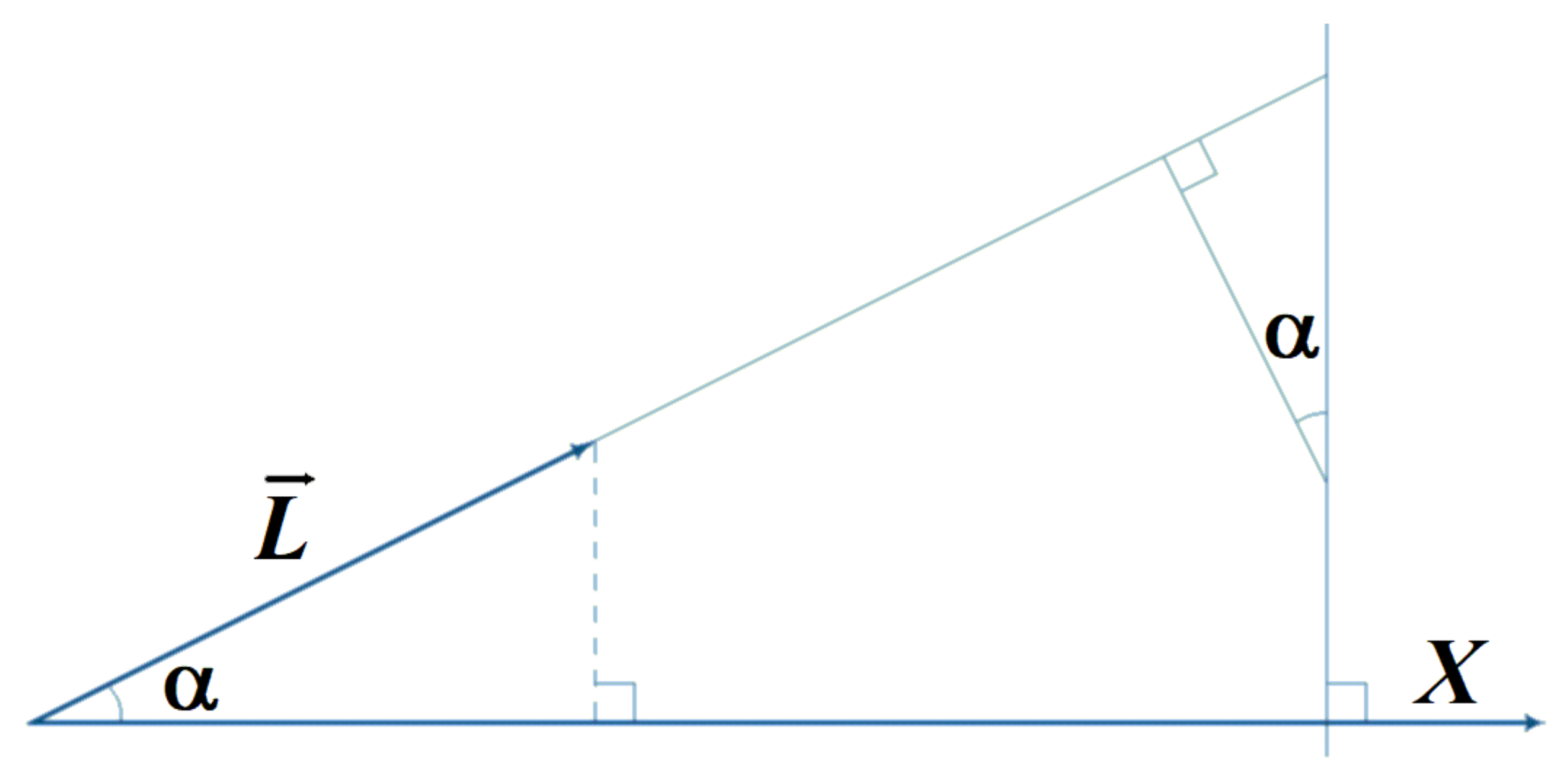
The first cosine is because the radiation is directed at an angle $\alpha$ to the X-axis and its speed in this direction is less (Figure 1). The second one is because the radiation falls to the surface perpendicular to the X-axis under the angle $\alpha$ and is distributed over a larger area. (The same 2/3 relate, for example, to the pressure with the average kinetic energy of the molecules).

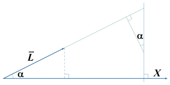
Figure 1. The origin of two cosines.

The heat flux density transmitted from one absolutely black flat surface with temperature $T_1$ to a parallel to its surface with temperature $T_2$ (12) when there is no medium between them is

$$J_{12}=2\sigma (T_1^4-T_2^4)/3.$$

(13)

Now let us consider the interaction of radiation with the medium. The probability of absorption characterises the medium. According to Booger’s law, the radiation absorbed in a transverse layer with a thickness of $\mathrm{d}h$ is proportional to the incident radiation

$$\mathrm{d}\overline{L}=-\overline{L}\mathrm{d}h/a.$$

(14)

According to Kirchhoff’s law, at thermal equilibrium, the absorbed radiance is equal to the emitted one

$$\mathrm{d}{\overline{L}}_{e-}=\mathrm{d}\overline{L}.$$

(15)

The absorption of the medium in the forward and reverse directions is the same in magnitude

$$\mathrm{d}{\overline{L}}_{e+}=-\mathrm{d}{\overline{L}}_{e-}.$$

(16)

If the radiation falls on the layer at an angle $\alpha$, then the absorption is inversely proportional to the cosine of the angle of incidence

$$\mathrm{d}h=\mathrm{d}x/cos\alpha .$$

(17)

On the contrary, the X-component of the radiance is directly proportional to the cosine of the angle of incidence. The change of the X-components of L is the same regardless of the direction of propagation

$${\left(\mathrm{d}L\right)}_x=-L\mathrm{d}x/a.$$

(18)

The area over which the incident on the medium layer at an angle $\alpha$ radiation falls is inversely proportional to the cosine $\alpha$. When calculating the integral X-component of the absorption (radiosity) of the layer, we must multiply this cosine by the square of the cosine (since again, as in Formula (12), we integrate over all spatial components)

$$\mathrm{d}J={\int }_0^{\pi /2}{cos}^3\alpha \mathrm{d}L\mathrm{d}\mathsf{\Omega }=-J\mathrm{d}x/a.$$

(19)

For the directed movement of heat by the radiation, Booger’s law is valid. The absorbed power is proportional to the incident power and the probability of absorption is proportional to the thickness of the medium layer.

Then (12), (15) the radiosity of the layer with thickness $\mathrm{d}x$ is

$$\mathrm{d}{J}_e=2\sigma T^4\mathrm{d}x/\left(3a\right).$$

(20)

We will note several established essential facts.

• With radiant heat transfer in a given direction, the diffuse type of radiation does not complicate this process. All spatial components of the radiation change equally in the direction of propagation. For the absorption of a layer of thickness $\mathrm{d}x$ normal to a given direction, the Booger’s law (19) is valid.
• For the radiosity of a layer with a thickness of $\mathrm{d}x$, the Formula (20) is valid. It does not matter how heat is transferred to this layer and even whether the layer temperature is constant at this time or changes. The radiosity of the layer is the same exactly. It is an inherent property of the layer with a temperature of T.
• For the validity of Formulas (19) and (20), there is no condition of a large optical thickness of the medium. The diffuse approximation is a more general approach than the radiant thermal conductivity approximation. Formulas (19) and (20) are applicable for calculating the heat transfer in a medium with a known dependence of its temperature on the coordinate.

Let us find the visibility of a layer with a temperature T and a thickness $\mathrm{d}x$ at a distance x from it (the fraction of radiosity reaching this place directly from that layer). We integrate (19) and get

$$\mathrm{d}{J}_x=\mathrm{d}{J}_{e}exp\left(\frac{-x}{a}\right)=2\sigma T^{4}exp\left(\frac{-x}{a}\right)\frac{\mathrm{d}x}{3a}.$$

(21)

2.2. Radiant Thermal Conductivity of a Grey Medium

Suppose there is a small temperature gradient $\nabla T$ directed along the X-axis in the medium. Furthermore, it is such that the temperature change on the thickness a is small compared to the temperature itself

$$\nabla T=\mathrm{d}T/\mathrm{d}x\ll T/a.$$

(22)

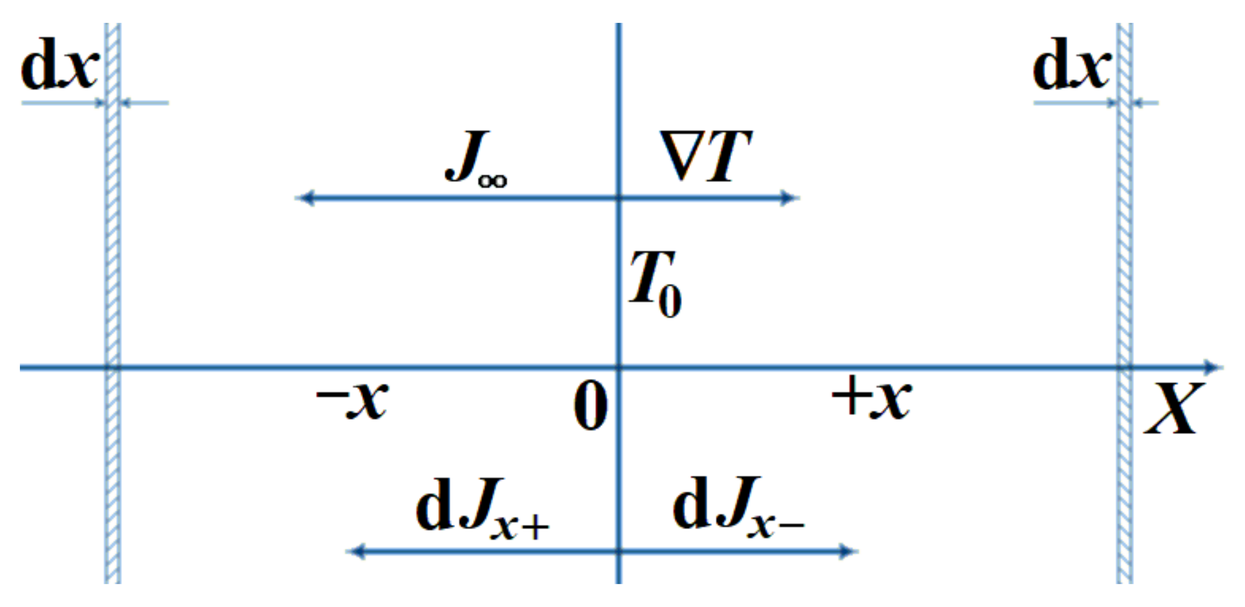
Let us find the heat flux density passing through the plane with the temperature $T_0$ and the coordinate $x=0$. In this case, the heat flux from the hot side from it does not compensate the flux from the cold side (Figure 2). The heat flux density $\mathrm{d}{J}_{x\pm }$ from layers with a thickness $\mathrm{d}x$ located at a distance $\pm x$ from the plane (21) is

$$\mathrm{d}{J}_{x\pm }=\mp 2\sigma {\left(T_0\pm x\nabla T\right)}^{4}exp(-\left|x\right|/a)\mathrm{d}x/\left(3a\right).$$

(23)

Figure 2. Integrating of radiation contributions from all layers of the medium.

The uncompensated heat flux density is equal to the sum of the flux densities from the cold and hot sides of the plane

$$J_{\infty }={\int }_0^{\infty }(\mathrm{d}{J}_{x+}+\mathrm{d}{J}_{x-}).$$

(24)

We will call it $J_{\infty }$, because such flux density is obtained when stationary heat transfer and a large optical thickness of the medium occur. Taking into account (22),

$${\left(T_0+x\nabla T\right)}^4-{\left(T_0-x\nabla T\right)}^4=8T_0^{3}x\nabla T-8T_0{(x\nabla T)}^3\approx 8T_0^{3}x\nabla T.$$

(25)

Since all odd terms are mutually deleted, the accuracy of the application of the radiant thermal conductivity approximation

$$\delta \sim {(a\nabla T/T_0)}^2.$$

(26)

In the linear approximation, we get

$$J_{\infty }=-\frac{16\sigma T_0^3\nabla T}{3a}{\int }_0^{\infty }xexp\left(\frac{-x}{a}\right)\mathrm{d}x=-\frac{16\sigma T_0^{3}a\nabla T}{3}=-R\nabla T.$$

(27)

This formula entirely coincides with Formulas (4) and (5). In addition, we found that the radiant thermal conductivity approximation is valid with the condition (22) and with the accuracy (26). The approximation of the radiant thermal conductivity is applicable when the curvature radius of the constant temperature surface is much larger than a.

2.3. Radiosity of a Thin Layer of a Medium with an Arbitrary Frequency Dependence of Scattering and Absorption

Now we obtain the relations for a medium with an arbitrary frequency dependences of absorption $a_a\left(\omega \right)$ and scattering $a_s\left(\omega \right)$.

Spectral flux density $e\left(\omega \right)$ is

$$\overline{e}\left(\omega \right)=\mathrm{d}\overline{E}/\mathrm{d}\omega .$$

(28)

In thermal equilibrium, radiation propagates in any direction with a spectral radiance l that depends only on the frequency

$$\overline{l}\left(\omega \right)=\mathrm{d}\overline{L}/\mathrm{d}\omega =\mathrm{d}\overline{e}/\mathrm{d}\mathsf{\Omega }=\mathrm{Const}.$$

(29)

The integral X-component of the spectral flux density j is

$$j={\int }_0^{\pi /2}l{cos}^2\alpha \mathrm{d}\mathsf{\Omega }=\mathrm{d}J/\mathrm{d}\omega .$$

(30)

For the spectral density of black body radiant flux f is valid

$${\int }_0^{\infty }f(\omega ,T)\mathrm{d}\omega =\sigma T^4.$$

(31)

Then

$$j=2f/3.$$

(32)

The medium is characterised by the probability of absorption

$$\mathrm{d}\overline{l_a}/\mathrm{d}h=-\overline{l}/a_a.$$

(33)

The medium is also characterised by the probability of scattering

$$\mathrm{d}\overline{l_s}/\mathrm{d}h=-\overline{l}/a_s.$$

(34)

Therefore,

$$\mathrm{d}\overline{l}/\mathrm{d}h=\mathrm{d}\overline{l_a}/\mathrm{d}h+\mathrm{d}\overline{l_s}/\mathrm{d}h=-l/a.$$

(35)

And

$$a^{-1}=a_a^{-1}+a_s^{-1}.$$

(36)

According to Kirchhoff’s law, at thermal equilibrium, the absorbed spectral flux density by the medium element is equal to the emitted one. The transparency of the medium element in the forward and reverse direction is also the same

$$\mathrm{d}{\overline{l}}_a=\mathrm{d}{\overline{l}}_{ae-}=-\mathrm{d}{\overline{l}}_{ae+}.$$

(37)

Formula (37) is a form of the law of conservation of energy. In the same form, this law is also valid for scattering

$$\mathrm{d}{\overline{l}}_s=\mathrm{d}{\overline{l}}_{se-}=-\mathrm{d}{\overline{l}}_{se+}.$$

(38)

Therefore,

$$\mathrm{d}\overline{l}=\mathrm{d}{\overline{l}}_{e-}=-\mathrm{d}{\overline{l}}_{e+}.$$

(39)

With the diffuse approximation, in the state of thermal equilibrium of radiation with the medium, including with stationary heat transfer, the contributions of scattering and absorption-emission are additive and symmetric. When it is important how much heat the medium receives and how its temperature changes, the differences appear in dynamics.

For the spatial components of the spectral flux density (l, $\mathrm{d}l$), completely similar conditions (29), (35), (39) are met as for the spatial components of the flux density (L, $\mathrm{d}L$) in the case of a grey medium (7), (14)–(16). In particular, it is also true that in the direction of the X-axis, all the spatial components of the spectral flux density change equally

$${\left(\mathrm{d}l\right)}_x=-l\mathrm{d}x/a.$$

(40)

Then for the integral X-component of the spectral absorption (spectral radiosity) of the layer following equation is valid

$$\mathrm{d}j=-j\mathrm{d}x/a.$$

(41)

The spectral radiosity of the layer with thickness $\mathrm{d}x$ (31) is

$$\mathrm{d}{j}_e=2f\mathrm{d}x/\left(3a\right).$$

(42)

The spectral visibility of the layer (the fraction of spectral radiosity reaching this place directly from that layer) with temperature T and thickness $\mathrm{d}x$ at a distance x from it is

$$\mathrm{d}{j}_x=\mathrm{d}{j}_{e}exp\left(-x/a\right)=2fexp\left(-x/a\right)\mathrm{d}x/\left(3a\right).$$

(43)

The last three formulas are again particularly noteworthy. We obtained formulas for the spectral radiosity and visibility of a thin layer of a medium in the diffuse approximation from the first principles without making unnecessary restrictions. For the spectral flux density in a medium with an arbitrary frequency dependence of scattering and absorption, the same relations as in the case of flux density in a grey medium (19)–(21) are obtained. All spatial components of the spectral flux density, despite the diffuse radiation, also change equally. Therefore, the task about directed heat transfer is one-dimensional. Booger’s law is valid in the same form ((41) and (19)). The spectral radiosity is an inherent property of the medium layer with a temperature of T and penetration depth $a\left(\omega \right)$. Formulas (42) and (43) are applicable for calculating the heat transfer in a medium with a known dependence of its temperature on the coordinate. However, there is one more possibility of heat transfer from one spectral component to another.

2.4. Radiant Thermal Conductivity of a Medium with an Arbitrary Frequency Dependence of Scattering and Absorption

Suppose a small temperature gradient is directed along the X-axis in the medium and the condition (22) is fulfilled. The heat flux from the cross-sectional plane hot side of the medium with temperature $T_0$ also does not compensate for the flux from the cold side. We can only use a linear term of approximation of the function f on temperature

$$f\left(T\right)\approx f\left(T_0\right)+x\nabla T\mathrm{d}f/\mathrm{d}T.$$

(44)

We denote:

$$f^{\prime }=\mathrm{d}f/\mathrm{d}T.$$

(45)

The uncompensated flux density (23), (43)–(45) is equal to the sum of the flux densities from the cold and hot sides of the cross-sectional plane

$$\begin{array}{cc}\hfill J_{\infty }& ={\int }_0^{\infty }{\int }_0^{\infty }(\mathrm{d}{j}_{x+}+\mathrm{d}{j}_{x-})\mathrm{d}\omega \approx -\frac{4\nabla T}{3}{\int }_0^{\infty }\left({\int }_0^{\infty }xexp\left(\frac{-x}{a}\right)\mathrm{d}x\right)f^{\prime }\mathrm{d}\omega \hfill \\ \hfill & =-\frac{4\nabla T}{3}{\int }_0^{\infty }a{f}^{\prime }\mathrm{d}\omega .\hfill \end{array}$$

(46)

According to (31), (45)

$${\int }_0^{\infty }{f}^{\prime }\mathrm{d}\omega =4\sigma T_0^3.$$

(47)

We introduce the average penetration depth of thermal radiation

$$⟨a⟩=\left({\int }_0^{\infty }a\left(\omega \right)f^{\prime }\mathrm{d}\omega \right)/\left(4\sigma T_0^3\right).$$

(48)

Then

$$J_{\infty }=-\left(16\sigma T_0^3⟨a⟩/3\right)\nabla T=-R\nabla T.$$

(49)

When averaging the penetration depth, as a distribution function, it needs to use not the Planck function for spectral density of black body radiant flux but its derivative for absolute temperature. The spectrum parts with the largest radiation penetration depth make the most contribution to the radiative heat transfer. It is worth noting that we have a very one-sided idea about the transparency of gases as until recently about the nearest moon. We only know how gases absorb the radiation, and we know almost nothing about how transparent they are [11].

2.5. Problem Formulation

The spectral flux density (46) is directly proportional to the penetration depth

$$j_{\infty }=\mathrm{d}{J}_{\infty }/\mathrm{d}\omega =-4f^{\prime }a\nabla T/3.$$

(50)

We will use this direct proportionality. It is convenient to consider spectral components with a large heat transfer as hotter and introduce the concept of the temperature of the spectral component of radiation. For the radiation passing through a layer in thermal equilibrium with it, the temperature of the component is

$${\tau }_0\left(\omega \right)=a\left(\omega \right)T_0/⟨a⟩.$$

(51)

The average value of the temperature $T_0$ of all spectral components corresponds to the state of thermal equilibrium

$$⟨{\tau }_0\left(\omega \right)⟩=\left({\int }_0^{\infty }{\tau }_0\left(\omega \right)f^{\prime }\mathrm{d}\omega \right)/\left(4\sigma T_0^3\right)=T_0.$$

(52)

Formulas (27) and (49) are correct for the large optical thickness of the medium when the distance from its boundaries is much more than a. However, Formulas (19)–(21) and (41)–(43) are valid near the diffusely emitting (reflecting) boundaries of the medium too. They allow us to solve the inverse problem: to restore the dependence of the heat flux density on the coordinate based on the assumed dependence of the medium temperature on the coordinate. Additional conditions may follow from comparing the restored dependence with the dependence that we suppose to get when solving the problem. If these conditions were satisfied, then the proposed dependence of the medium temperature on the coordinate is the problem’s solution. Next, we will continue solving the problem of stationary heat transfer with a constant heat flux density in various versions of the formulation

$$J=\mathrm{Const}.$$

(53)

We have already obtained the simplest result $\nabla T$ = Const of solving this problem for radiative heat transfer at a large optical thickness of the medium, for which an additional condition $J=-R\nabla T$ (27), (49) is found. Now we will find the solution to this problem near the flat boundary of the medium.

3. Results

3.1. Radiative Heat Transfer Near an Opaque Surface

Suppose the medium fills a half-space bounded by an opaque diffusely reflecting and emitting plane with the same emissivity $\epsilon \left(\omega \right)$ and temperature $T_b$ over the entire plane. The heat flux density equal to $-R\nabla T$ is directed perpendicular to the plane along the X-axis. We assume that a difference between the spectral components of the radiation temperature jump $\tau \left(\omega \right)$ near the boundary exists. The average temperature (for the spectral components of radiation) of the medium near the plane is $T_0$. The temperature of the medium at a distance x from the plane is equal to T. For any frequency $\omega$ we look for a solution to the problem in the form

$$T=T_0+x\nabla T,T_0=⟨{\tau }_0\left(\omega \right)⟩,T_b={\tau }_0\left(\omega \right)+\tau \left(\omega \right).$$

(54)

Then (42), (43) we find at the frequency $\omega$ the spectral flux density at an arbitrary distance h from the plane

$$\begin{array}{c}\hfill j_h=\frac{2f^{\prime }}{3}\left(\epsilon \tau exp\frac{-h}{a}+{\int }_0^{h}x\nabla Texp\frac{-h+x}{a}\frac{\mathrm{d}x}{a}+{\int }_0^{\infty }x\nabla T(1-\epsilon )exp\frac{-h-x}{a}\frac{\mathrm{d}x}{a}\right)-\\ \hfill -\frac{2f^{\prime }}{3}{\int }_h^{\infty }x\nabla Texp\frac{h-x}{a}\frac{\mathrm{d}x}{a}=\frac{2f^{\prime }}{3}\left(-2a\nabla T+\left(\epsilon \tau +(2-\epsilon )a\nabla T\right)exp\frac{-h}{a}\right).\end{array}$$

(55)

The first independent of h term of the found spectral flux density corresponds to the expected spectral flux density of the heat (50). The second term must be equal to zero for any h. This imposes an additional condition, according to which the temperature jump (of the spectral component) that occurs near the surface must be equal to

$$\tau =-a\nabla T(2-\epsilon )/\epsilon .$$

(56)

Near an opaque surface, the radiation is not in thermal equilibrium with the medium. Nevertheless, the excess of energy brought by some parts of the spectrum compensates for the lack of energy that others do not bring. The medium itself, where the radiant heat transfer occurs, is in a state of thermal equilibrium. For $\tau$ satisfying (56), the heat flux density is $J=-R\nabla T$.

We see that the temperature jump $\tau$ is proportional to the spectral flux density. Therefore, the spectral density of the thermal conductance characterises the surface

$$\zeta =\frac{j}{\tau }=\frac{4}{3}{f}^{\prime }\frac{\epsilon }{2-\epsilon }.$$

(57)

Note that the obtained result does not include the characteristics of the medium. The spectral density of the thermal conductance depends only on the properties of the surface.

There is another way to obtain the same result. Let there be two parallel opaque planes with emissivity $\epsilon$, between which there is no medium and the temperatures are equal $T_0\pm \Delta T/2,\Delta T\ll T_0$. From the hot to the cold one, the spectral flux density $j_A$ goes and backwards the spectral flux density $j_B$. Then

$$j_A=\frac{2\epsilon }{3}\left(f+f^{\prime }\frac{\Delta T}{2}\right)+(1-\epsilon )j_B,j_B=\frac{2\epsilon }{3}\left(f-f^{\prime }\frac{\Delta T}{2}\right)+(1-\epsilon )j_A.$$

(58)

We subtract the second from the first equation. Then we can find that the spectral flux density going from one flat surface to another is

$$j=j_A-j_B=\frac{2}{3}{f}^{\prime }\Delta T\frac{\epsilon }{2-\epsilon }.$$

(59)

Since we have two flat surfaces, for each of them we get the same spectral density of thermal conductance as before

$$\zeta =\frac{2j}{\Delta T}=\frac{4}{3}{f}^{\prime }\frac{\epsilon }{2-\epsilon }.$$

(60)

This example confirms the correctness of our method for obtaining the Formula (57).

We integrate (57,60) over the entire frequency spectrum (47). Thus, we find the thermal conductance of a flat surface

$$Z=\frac{16}{3}\sigma T_0^3⟨\frac{\epsilon }{2-\epsilon }⟩,\mathrm{where}$$

(61)

$$⟨\frac{\epsilon }{2-\epsilon }⟩=\left({\int }_0^{\infty }\frac{\epsilon }{2-\epsilon }{f}^{\prime }\mathrm{d}\omega \right)/\left(4\sigma T_0^3\right).$$

(62)

When averaging, as a distribution function, it also needs to use not the Planck function for spectral density of black body radiant flux but its absolute temperature derivative.

In fact, we have once again confirmed the well-known Christiansen formula that says that any surface preventing the passage of radiation introduces additional thermal resistance (inverse to thermal conductance Z). In addition, we obtained this thermal resistance for diffuse surface with an arbitrary frequency dependence of emissivity.

3.2. Radiative Heat Transfer Near the Boundary of a Medium and Free Space

Let us solve Problem (53) when all the radiation leaving the medium goes away and nothing returns. This means that the temperature of the free space is equal to absolute zero. We will assume that the temperature of the outer boundary of the medium is $T_0$. We will assume too that the temperature of the medium increases linearly with the distance from the boundary

$$T=T_0+\gamma x,T_0=⟨{\tau }_0\left(\omega \right)⟩,$$

(63)

where $\gamma =-J/R$ is the temperature gradient formed at such a heat flux density in the depth of the medium. Then in (22), (42), (43), we find the spectral flux density at an arbitrary distance h from the boundary

$$\begin{array}{cc}\hfill j_h& =\frac{2}{3}\left({\int }_0^{h}f\left(T\right)exp\frac{-h+x}{a}\frac{\mathrm{d}x}{a}-{\int }_h^{\infty }f\left(T\right)exp\frac{h-x}{a}\frac{\mathrm{d}x}{a}\right)=\hfill \\ \hfill & =\frac{2}{3}\left(-2f^{\prime }\gamma a+\left(f\left(T_0\right)-f^{\prime }\gamma a\right)exp\frac{-h}{a}\right).\hfill \end{array}$$

(64)

The independent of h term gives the expected (50) spectral flux density. The additional condition is

$$f\left(T_0\right)=f^{\prime }\gamma a.$$

(65)

It allows one to determine, corresponding to a given heat flux density, temperature of the outer boundary. We integrate (65) over the entire frequency spectrum

$$\sigma T_0^4=4\sigma T_0^3\gamma ⟨a⟩\Rightarrow T_0=4\gamma ⟨a⟩.$$

(66)

The spectral flux density beyond the boundary of the medium is

$$j=\frac{\mathrm{d}J}{\mathrm{d}\omega }=\frac{4f^{\prime }\gamma a}{3}=\frac{f^{\prime }{T}_{0}a}{3⟨a⟩}=\frac{f^{\prime }{\tau }_0}{3}.$$

(67)

In addition, we obtain the effective temperature $T_e$ of the leaving the medium radiation. We integrate (67) over the entire frequency spectrum

$$J=\frac{2\sigma T_e^4}{3}=\int \frac{f^{\prime }\gamma a\mathrm{d}\omega }{3}=\frac{16\sigma T_0^3\gamma ⟨a⟩}{3}=\frac{4\sigma T_0^4}{3}.$$

(68)

Then

$$T_e=T_0\sqrt[4]{2}.$$

(69)

Let us show the possibilities of applying the obtained relations on the example of evaluating the characteristics of the thermal transparency of our planet atmosphere. The solar energy flux density near the Earth is equal to $J_S=$ 1370 W/m² [12]. The albedo is about 40%. Therefore, a heat flux density from the Earth’s surface into outer space is $J_E=(2/3)·0.6J_S/4=$ 137 W/m². Since the depth of radiation penetration is inversely proportional to the density of the medium, we apply the approximation of the atmosphere by a layer with a constant density equal to the density of air at the sea level. The thickness of this layer is $H=$ 8434 m. From (68), (69), the temperature of the Earth’s radiation is $T_e=$ 245 K, and the temperature of the outer boundary of the atmosphere is $T_0=$ 206 K. The average air temperature at the Earth’s surface $T_E=$ 288 K. Since the temperature difference $\Delta T=T_E-T_0=$ 82 K is small compared to the average temperature of the atmosphere $T_a=(T_E+T_0)/2=$ 247 K, we can estimate from (49) the average depth of thermal radiation penetration. At the sea level, it is equal to

$$⟨a⟩=\frac{J_{E}H}{16\sigma T_a^3\Delta T/3}\approx 3 \mathrm{km}.$$

(70)

At a larger difference, we need to consider the nonlinearity of the temperature dependence on the height.

Of course, it is a very rough estimate. However, it allows us to understand the nature of the change in air temperature with altitude. At radiative heat transfer near human objects, whose dimensions are usually less than 3 km, the diffuse approximation is not applicable. Only $exp(-H/⟨a⟩)\approx 5\%$ of the radiation goes to the upper boundary of the atmosphere directly from the Earth’s surface. Even for an atmosphere as thin as the Earth’s, the spectrum of thermal radiation (67) is almost entirely determined by the properties of its constituent gases. Note that almost all the parameters used for the estimation can be obtained remotely using astronomical measurements.

3.3. Radiative–Conductive Heat Transfer in a Grey Medium Near a Grey Surface

Radiative–conductive heat transfer around us is rare. Most often, it can be observed in light heat-protective materials [13,14]. However, it can be performed under laboratory conditions in gases. To do this, we must place the heater strictly above the refrigerator. It is easier to carry out measurements at high pressure, to which the depth of radiation penetration (the radiative component of thermal conductivity) is inversely proportional. The conductive component of thermal conductivity is almost independent of pressure. At a high pressure, both components are comparable.

Let us proceed to the solution of the Problem (53) for radiative–conductive heat transfer. Let us first consider the more straightforward case of a grey medium with a penetration depth of a and a diffuse grey flat surface with an emissivity of $\epsilon$. With a large optical thickness of a medium, the problem has an obvious solution (2), (4), (27)

$$J_{\infty }=J_{R\infty }+J_{C\infty }=-(R+C)\nabla T=-\lambda \nabla T.$$

(71)

The total thermal conductivity of the medium $\lambda$ is the sum of the radiative and conductive components. A stationary parallel heat flux with a density J propagates into the medium perpendicular to the surface with a temperature of $T_0+T_h(T_h\ll T_0)$. That formed away from the surface temperature gradient is

$$\gamma =-J/\lambda .$$

(72)

With the condition (22), we look for the temperature dependence on the distance from the surface in the form

$$T=T_0+\gamma x+T_h·exp(-x/b).$$

(73)

Then the radiative component of the flux density at a distance h from the surface is

$$\begin{array}{cc}\hfill J_{Rh}& =\frac{2\sigma }{3}\left({\int }_0^h\frac{e^{\frac{x-h}{a}}{T}^4\mathrm{d}x}{a}-{\int }_h^{\infty }\frac{e^{\frac{h-x}{a}}{T}^4\mathrm{d}x}{a}+{\int }_h^{\infty }\frac{e^{\frac{-h-x}{a}}{T}^4(1-\epsilon )\mathrm{d}x}{a}+\epsilon {(T_0+T_h)}^4{e}^{\frac{-h}{a}}\right)\hspace{1em}\approx \hfill \\ & \approx J_{R\infty }\left(1-\frac{2-\epsilon }{\epsilon }{e}^{\frac{-h}{a}}+\frac{T_h}{b\gamma }\left(\frac{-1}{{(a/b)}^2-1}{e}^{\frac{-h}{b}}+\frac{1+(a/b-1)\epsilon /2}{{(a/b)}^2-1}{e}^{\frac{-h}{a}}\right)\right).\hfill \end{array}$$

(74)

The conductive component of the flux density at a distance h is equal to

$$J_{Ch}=-C\left(\gamma -\frac{T_h}{b}{e}^{\frac{-h}{b}}\right)=J_{C\infty }\left(1+\frac{T_h}{b\gamma }{e}^{\frac{-h}{b}}\right).$$

(75)

Since the total heat flux density should not depend on h, sums of the factors at $exp(-h/b)$ and $exp(-h/a)$ must be equal to 0.

$$\frac{-1}{{(a/b)}^2-1}\frac{R{T}_h}{b}+\frac{C{T}_h}{b}=0 \mathrm{and}$$

(76)

$$-\frac{2-\epsilon }{\epsilon }+\frac{T_h}{b\gamma }\frac{1+(a/b-1)\epsilon /2}{{(a/b)}^2-1}=0.$$

(77)

From Equation (76)

$${\left(\frac{a}{b}\right)}^2=\frac{J_{\infty }}{J_{C\infty }}=\frac{R+C}{C},b=a\sqrt{\frac{C}{R+C}}=a\beta .$$

(78)

From Equation (77)

$$T_h=-\frac{b\gamma \left({(a/b)}^2-1\right)}{1+(a/b)\epsilon /(2-\epsilon )}=-\frac{a\gamma (1-{\beta }^2)}{\beta +\epsilon /(2-\epsilon )}.$$

(79)

The unambiguity of the obtained coefficients $T_h$ and b and the possibility of satisfying the condition (53) confirm the correctness of the chosen dependence (73). The coefficient b is the thickness of the radiative–conductive relaxation of the medium. It does not depend on the properties of the surface. Therefore, it is an inherent characteristic of the medium. That is why the relaxation thickness is the same not only near the opaque surface but also near other disturbances, for example, at the boundary with another medium. The coefficient $T_h$ is a temperature jump at a distant opaque surface.

The temperature jump is again proportional to the heat flux density. Therefore, the thermal conductance of the distant opaque surface is

$$Z=\frac{J}{T_h}=\frac{16}{3}\sigma T_0^3\frac{\beta +\epsilon /(2-\epsilon )}{{(1-{\beta }^2)}^2}.$$

(80)

3.4. Radiative–Conductive Heat Transfer in a Medium with an Arbitrary Frequency Dependence of Absorption and Scattering Near a Surface with an Arbitrary Frequency Dependence of Emissivity

Suppose a medium with an arbitrary frequency dependence of absorption and scattering (36) and the penetration depth of radiation $a\left(\omega \right)$ fill the half-space bounded by an opaque diffusely reflecting and emitting flat surface with the same emissivity $\epsilon \left(\omega \right)$ and temperature $T_b$

$$T_b{=T|}_{x=0}={\tau }_0\left(\omega \right)+\tau \left(\omega \right),T_0=⟨{\tau }_0\left(\omega \right)⟩.$$

(81)

The constant heat flux density $J=-\lambda \gamma$ is directed perpendicular to the surface along the X-axis. The temperature of the medium at a distance x from the surface is equal to T. At any frequency $\omega$, we look for a solution of the Problem (53) in the form:

$$T={\tau }_0+u(x,\omega ),u(x,\omega )=\gamma x+\tau ·exp(-x/b\left(\omega \right)).$$

(82)

Then (22), (42), (43) we find the radiative component of the spectral flux density at an arbitrary distance h from the plane

$$\begin{array}{cc}\hfill j_{Rh}& =\frac{2f^{\prime }}{3}\left({\int }_0^h\frac{e^{\frac{x-h}{a}}u\mathrm{d}x}{a}-{\int }_h^{\infty }\frac{e^{\frac{h-x}{a}}u\mathrm{d}x}{a}+{\int }_h^{\infty }\frac{e^{\frac{-h-x}{a}}u(1-\epsilon )\mathrm{d}x}{a}+\epsilon \tau e^{\frac{-h}{a}}\right)\hspace{1em}\approx \hfill \\ & \approx \frac{2f^{\prime }}{3}\left(-2a\gamma +\left(\frac{a\epsilon \tau }{a+b}+\frac{2\tau ab}{a^2-b^2}+a\gamma (2-\epsilon )\right)e^{\frac{-h}{a}}-\frac{2\tau ab}{a^2-b^2}{e}^{\frac{-h}{b}}\right).\hfill \end{array}$$

(83)

We introduce the concept of the conductive component of the spectral flux density

$$j_C=\mathrm{d}{J}_C/\mathrm{d}\omega =-\mathrm{d}(C\mathrm{d}T/\mathrm{d}x)/\mathrm{d}\omega .$$

(84)

Since (48), (52), (62) the distribution function is known to us

$$T=\left({\int }_0^{\infty }\left({\tau }_0+\gamma x+\tau ·exp(-x/b)\right)f^{\prime }\mathrm{d}\omega \right)/\left(4\sigma T_0^3\right).$$

(85)

Then at a distance h from the plane

$$j_{Ch}=-C{f}^{\prime }\left(\gamma -(\tau /b)exp(-h/b)\right)/\left(4\sigma T_0^3\right).$$

(86)

The total spectral flux density is

$$j_h=j_{Rh}+j_{Ch}.$$

(87)

When integrating j over the entire frequency spectrum, the independent of $exp(-h/a)$ and $exp(-h/b)$ terms give the expected heat flux density

$$J=-{\int }_0^{\infty }\left(\frac{4a}{3}+\frac{C}{4\sigma T_0^3}\right)\gamma f^{\prime }\mathrm{d}\omega =-(R+C)\gamma .$$

(88)

Hence, the factors at $exp(-h/b)$ and $exp(-h/a)$ must be equal to 0.

$$\frac{C}{4\sigma T_0^{3}b}{f}^{\prime }\tau -\frac{2}{3}{f}^{\prime }\tau \frac{2ab}{a^2-b^2}=0\mathrm{and}$$

(89)

$$\gamma (2-\epsilon )+\tau \left(\frac{\epsilon }{a+b}+\frac{2b}{a^2-b^2}\right)=0.$$

(90)

From (89) the thickness of the radiative–conductive relaxation of the radiation spectral component is

$$b=a\sqrt{\frac{C}{C+16\sigma T_0^{3}a/3}}=a\beta .$$

(91)

$\beta$ is the coefficient of radiative–conductive relaxation. From (90) the temperature jump of the radiation spectral component at the distant opaque surface is

$$\tau =-\frac{\gamma (a^2-b^2)}{b+a\epsilon /(2-\epsilon )}=-\frac{a\gamma (1-{\beta }^2)}{\beta +\epsilon /(2-\epsilon )}.$$

(92)

The fact that it was possible to uniquely determine the parameters b and $\tau$ and satisfy the condition (53) for any h confirms the correctness of the solution (82). From (91) $b<a$ and $\beta <1$ for any a. In the limit with C tending to zero, b also tends to zero, and $\tau$ corresponds to (56). The temperature jump $\tau$ is again (92) proportional to the spectral flux density j. Therefore, the spectral density of the thermal conductance of the distant opaque surface is

$$\zeta =\frac{j}{\tau }=\frac{4}{3}{f}^{\prime }\frac{\beta +\epsilon /(2-\epsilon )}{{(1-{\beta }^2)}^2}.$$

(93)

We integrate (93) over the entire frequency spectrum and find the thermal conductance of the distant opaque surface

$$Z=\frac{16}{3}\sigma T_0^3⟨\frac{\beta +\epsilon /(2-\epsilon )}{{(1-{\beta }^2)}^2}⟩,\mathrm{where}$$

(94)

$$⟨\frac{\beta +\epsilon /(2-\epsilon )}{{(1-{\beta }^2)}^2}⟩=\left({\int }_0^{\infty }\left(\frac{\beta +\epsilon /(2-\epsilon )}{{(1-{\beta }^2)}^2}\right)f^{\prime }\mathrm{d}\omega \right)/\left(4\sigma T_0^3\right).$$

(95)

If a and $\epsilon$, respectively, b and $\tau$ do not depend on the frequency, this solution reduces to what we obtained for the grey medium (78), (80).

3.5. Radiative–Conductive Heat Transfer in a Medium with an Arbitrary Frequency Dependence of Absorption and Scattering between Two Identical Parallel Surfaces with an Arbitrary Frequency Dependence of Emissivity

Suppose two identical parallel flat surfaces with diffuse emissivity $\epsilon \left(\omega \right)$ and temperatures $T_0\pm \Delta T/2,\Delta T\ll T_0$ are at a distance d. A medium with a conductive component of thermal conductivity C and a radiation penetration depth $a\left(\omega \right)$ is between them. From the hot surface to the cold one, along the X-axis, there is a radiative–conductive heat flux with a density of $J=-(R+C)\gamma$. The solution of Problem (53) is symmetric about a point equidistant from the planes, which we choose as the null of coordinates.

From (82), (86) near the surface, the temperature gradient is

$${\gamma }_{+}=\gamma -⟨\tau /b⟩=-J/C.$$

(96)

Only the conductive component of thermal conductivity determines it. This is true regardless of whether there is a second surface or not. b and $\tau$ found in (91, 92) are the parameters of radiative–conductive heat transfer. The same parameters should describe the process in the current task.

We look for a solution of the Problem (53) in the form

$$T=⟨u(x,\omega )⟩=T_0+\gamma x+⟨\psi (d,\omega )\tau \left(exp\left(\right(-x-d/2)/b)-exp\left(\right(x-d/2)/b)\right)⟩.$$

(97)

u is the temperature of the spectral component of the radiation (51). $\psi$ is a coefficient that expresses the mutual influence of surfaces. We calculate the temperature derivative by the coordinate at $x=\pm d/2$ and substitute to (96). Then we obtain

$$\psi ={\left(1+exp(-d/b)\right)}^{-1}.$$

(98)

The temperature difference of the spectral components at $x=\pm d/2$ is

$$\Delta u=u(d/2)-u(-d/2)=\gamma d-2\tau ·tanh(d/(2b\left)\right).$$

(99)

The spectral density of the thermal conductance from one surface to another (88, 91) is

$$\zeta =\frac{j}{\Delta u}=\frac{\mathrm{d}J/\mathrm{d}\omega }{\Delta u}=\frac{4}{3}{f}^{\prime }{\left(\frac{d(1-{\beta }^2)}{a}+\frac{2{(1-{\beta }^2)}^2}{\beta +\epsilon /(2-\epsilon )}tanh\frac{d}{2a\beta }\right)}^{-1}.$$

(100)

We integrate (100) over the entire frequency spectrum and find the thermal conductance from one surface to another

$$Z=\frac{16}{3}\sigma T_0^3⟨{\left(\frac{d(1-{\beta }^2)}{a}+\frac{2{(1-{\beta }^2)}^2}{\beta +\epsilon /(2-\epsilon )}tanh\frac{d}{2a\beta }\right)}^{-1}⟩,\mathrm{where}$$

(101)

$$\begin{array}{c}\hfill ⟨{\left(\frac{d(1-{\beta }^2)}{a}+\frac{2{(1-{\beta }^2)}^2}{\beta +\epsilon /(2-\epsilon )}tanh\frac{d}{2a\beta }\right)}^{-1}⟩=\\ \hfill =\left({\int }_0^{\infty }{\left(\frac{d(1-{\beta }^2)}{a}+\frac{2{(1-{\beta }^2)}^2}{\beta +\epsilon /(2-\epsilon )}tanh\frac{d}{2a\beta }\right)}^{-1}{f}^{\prime }\mathrm{d}\omega \right)/\left(4\sigma T_0^3\right).\end{array}$$

(102)

At a small conductive component of the thermal conductivity $\beta \ll 1$ and a large distance between the surfaces $d\gg 2a\beta$,

$$Z\approx ⟨{\left(\frac{2}{16\sigma T_0^3/3}\frac{2-\epsilon }{\epsilon }+\frac{d}{C+16\sigma T_0^{3}a/3}\right)}^{-1}⟩.$$

(103)

The spectral density of the thermal resistance of the system consists of the spectral densities of the resistances of two boundaries (61) and the resistance of the medium layer (71) between them. Note that it is not necessary to fulfil the condition of a large optical thickness of the medium $d\gg a$ in this case.

On the contrary, at a small distance between the surfaces $d\ll 2a\beta$,

$$Z\approx \frac{C}{d}⟨\frac{\beta +\epsilon /(2-\epsilon )}{\beta +{\beta }^2\epsilon /(2-\epsilon )}⟩.$$

(104)

Then, at a significant contribution of the conductive component $\beta \sim 1$ and a significant reflection from the surfaces $\epsilon \ll 2\beta$, the radiative component of the heat flux from one surface to another can be neglected, and $Z\approx C/d$. The latter helps measure the conductive component of the thermal conductivity of gases, which is poorly known too.

Measurements of the dependence $Z\left(d\right)$ at a mid $d(d\sim 2a\beta )$ and a grey surface ($\epsilon =$ Const) with appropriate mathematical processing will give a probabilistic spectrum of depths of the radiative–conductive relaxation. Using surfaces with a known dependence $\epsilon \left(\omega \right)$, we can also get information about a frequency dependence of the depth of radiation penetration. Note once again that measurements of radiative–conductive heat transfer (without convection) are relatively easy to implement [13,14].

4. Conclusions

Thus, we solved several useful problems analytically on stationary radiative and radiative–conductive heat transfer in a medium with an arbitrary frequency dependence of absorption and scattering near boundaries with different emissivity. The obtained boundary conditions help study and understand the properties of both the boundaries themselves and the media near them. The solutions can be applied to analyse the composition and density of macroscopic gas objects. The solution of the latter problem is the theoretical basis for measuring the transparency of the gases (large depths of penetration).

Recently, many thermal physics schools have formed a dangerous opinion that using the diffuse approximation is useless for this science. We should note that to think so is like rejecting the second law of thermodynamics. From our point of view, a more correct approach is to understand where the diffuse approximation is valid and study relaxation processes.

References

- Howell, J.R.; Siegel, R. Thermal Radiation Heat Transfer; NASA: Washington, WA, USA, 1971.
- Viskanta, R.; Grosh, R.J. Heat transfer by simultaneous conduction and radiation in an absorbing medium. J. Heat Transfer 1962, 84, 63–72. [Google Scholar] [CrossRef]
- Doornink, D.G.; Hering, R.G. Transient Combined Conductive and Radiative Heat Transfer. J. Heat Transf. 1962, 9, 473–478. [Google Scholar] [CrossRef]
- Moore, T.J.; Jones, M.R. Analysis of the conduction–radiation problem in absorbing, emitting, non-gray planar media using an exact method. Int. J. Heat Mass Transf. 2014, 73, 804–809. [Google Scholar] [CrossRef] [Green Version]
- Perraudin, D.Y.S.; Haussener, S. Numerical quantification of coupling effects for radiation-conduction heat transfer in participating macroporous media: Investigation of a model geometry. Int. J. Heat Mass Transfer 2017, 112, 387–400. [Google Scholar] [CrossRef] [Green Version]
- Sun, S.-C.; Qi, H.; Wang, S.-L.; Ren, Y.-T.; Ruan, L.-M. A multi-stage optimization technique for simultaneous reconstruction of infrared optical and thermophysical parameters in semitransparent media. Infrared Phys. Technol. 2018, 92, 219–233. [Google Scholar] [CrossRef]
- Sans, M.; Schick, V.; Parent, G.; Farges, O. Experimental characterization of the coupled conductive and radiative heat transfer in ceramic foams with a flash method at high temperature. Int. J. Heat Mass Transf. 2020, 148, 119077. [Google Scholar] [CrossRef] [Green Version]
- Fan, C.; Li, X.L.; Xia, X.L.; Sun, C. Tomography-based pore level analysis of combined conductive-radiative heat transfer in an open-cell metallic foam. Int. J. Heat Mass Transf. 2020, 159, 120122. [Google Scholar] [CrossRef]
- Mironov, R.A.; Zabezhailov, M.O.; Cherepanov, V.V.; Rusin, M.Y. Transient radiative-conductive heat transfer modeling in constructional semitransparent silica ceramics. Int. J. Heat Mass Transfer 2018, 127, 1230–1238. [Google Scholar] [CrossRef]
- Cheng, X.; Liang, X. Analyses of coupled steady heat transfer processes with entropy generation minimization and entransy theory. Int. J. Heat Mass Transfer 2018, 127, 1092–1098. [Google Scholar] [CrossRef]
- Cormier, J.G.; Ciurylo, R.; Drummond, J.R. Cavity ringdown spectroscopy measurements of the infrared water vapor continuum. J. Chem. Phys. 2002, 116, 1030–1034. [Google Scholar] [CrossRef] [Green Version]
- Allen, C.W. Astrophysical Quantities; The Athlone Press: London, UK, 1973. [Google Scholar]
- Shamparov, E.Y. Heat Transfer in a Semitransparent Medium. Tech. Phys. 2018, 63, 133–140. [Google Scholar] [CrossRef]
- Shamparov, E.Y.; Bugrimov, A.L.; Rode, S.V.; Jagrina, I.N. Contribution of radiant component to thermal conductivity of the medium. J. Physics Conf. Ser. 2020, 1697, 012055. [Google Scholar] [CrossRef]
Publisher’s Note: MDPI stays neutral with regard to jurisdictional claims in published maps and institutional affiliations. |
© 2021 by the authors. Licensee MDPI, Basel, Switzerland. This article is an open access article distributed under the terms and conditions of the Creative Commons Attribution (CC BY) license (https://creativecommons.org/licenses/by/4.0/).