Ray Effects and False Scattering in Improved Discrete Ordinates Method

Abstract

The improved discrete ordinates method (IDOM) developed in our previous paper is extended to solve radiative transfer in three-dimensional radiative systems with anisotropic scattering medium. In IDOM, radiative intensities in a large number of new discrete directions are calculated by direct integration of the conventional discrete ordinates method (DOM) results, and radiative heat flux is obtained by integrating radiative intensities in these new discrete directions. Ray effects and false scattering, which tend to compensate each other, are investigated together in IDOM. Results show that IDOM can mitigate both of them effectively with high computation efficiency. Finally, the effect of scattering phase function on radiative transfer is studied. Results of radiative heat flux at boundaries containing media with different scattering phase functions are compared and analyzed. This paper indicates that the IDOM can overcome the shortages of the conventional DOM well while inheriting its advantages such as high computation efficiency and easy implementation.

1. Introduction

Efficient and precise solutions for radiative heat transfer are essential for thermal analysis in high-temperature processes, such as combustion, solar energy utilities, etc. Many numerical methods are employed to solve the radiative transfer equation (RTE). Among these, the discrete ordinates method (DOM) is widely used due to its high computation efficiency and easy implementation [1,2]. However, the accuracy of the DOM is affected by ray effects and false scattering [3,4,5], which are related to the angular and spatial discretization, respectively.

The most straightforward approaches for mitigating ray effects and false scattering are to increase discrete directions and refine spatial grids, respectively. Unfortunately, these approaches are computationally expensive due to increased computation time and memory. To use more accurate spatial discretization schemes is another common way to reduce false scattering [6,7,8]. The performance of several schemes including the upwind, central, hybrid, exponential, and high-resolution SMART schemes have been comprehensively compared by Liu et al. [6] to predict radiative intensity as well as radiative heat flux. Jessee and Fiveland [7] applied several bounded, high-resolution schemes to DOM, and the investigated schemes showed obvious improvement in accuracy over the standard step scheme. A later paper by Coelho [8] showed that bounded skew high-resolution schemes had better accuracy compared with the standard high-resolution schemes, yet with higher computational requirements. Besides, the double rays method is developed by Li et al. [9] to reduce false scattering error. In order to treat collimated irradiation, Li additionally used a hybrid spatial differencing scheme to reduce false scattering in arbitrarily specified discrete directions [10].

In terms of ray effects, in addition to increase discrete directions, to modify direction layout is another common remedy [11,12,13,14,15]. Numerical experiments have been conducted by Li et al. [11] showing that ray effects can be reduced by modifying direction layouts, and three corresponding countermeasures were proposed in their paper. Tencer [12] proposed a ray effects mitigation technique by averaging the computed results of various direction layouts, which are generated by arbitrarily rotating the reference layout. Quadrature rotation was also applied to solve time-dependent transport and results showed that ray effects were reduced significantly, including for small numbers of quadrature points [13]. Recently, goal-oriented angular adaptive algorithm was also utilized to mitigate ray effects [14,15]. However, neither increasing discrete directions nor modifying direction layout is a partially effective remedy for ray effects [16,17]. Several modifications to the discrete ordinates scheme were also proposed to eliminate ray effects. Lathrop [16] converted the discrete ordinates equation into a spherical harmonic-like equation to eliminate ray effects. A modification of the discrete ordinates named artificial scattering was proposed to mitigate ray effects [18]. Results demonstrated that artificial scattering yielded better accuracy than the traditional DOM with the same number of discrete ordinates. A modified discrete ordinates method (MDOM) has also been developed to mitigate ray effects caused by non-uniform emission of boundaries [19,20]. Coelho [21] extended the MDOM to reduce ray effects originated from non-uniform emission of the boundaries as well as the media. A similar concept was also applied to YIX method to mitigate ray effects [22]. Huang et al. [23] developed an improved discrete ordinate method (IDOM) based on the discrete ordinates scheme with infinitely small weight (DOS+ISW) concept [24]. Radiative intensities in a large number of new discrete directions are calculated by direct integration of the conventional DOM results. Several cases with isotropic scattering media were studied. Results showed that the IDOM can mitigate ray effects effectively with negligible computation time increased comparing with the conventional DOM.

In the papers mentioned above, ray effects and false scattering are resolved separately with different strategies. However, it is reported that there is an interaction between these two errors and that they tend to compensate each other [21,25,26]. That is to say, reducing one error while keeping the other unchanged may make the accuracy of final results worse. Then, in order to evaluate the performance of strategies applied to the DOM, ray effects and false scattering need to be considered at the same time. However, to the best of our knowledge, there is no previous work proposing or discussing a strategy that mitigates ray effects and false scattering concurrently.

In this paper, the IDOM is extended to solve radiative transfer in three-dimensional systems with anisotropic scattering medium. Ray effects, as well as false scattering, in the IDOM are investigated. First, the description of the IDOM is given. Then, ray effects and false scattering in the IDOM are studied by comparing the calculated radiative heat flux with the benchmark solution provided by the reverse Monte Carlo (RMC) method. Finally, the effect of scattering phase function on radiative transfer is studied by the IDOM.

2. The Improved Discrete Ordinates Method

In this section, a brief description of the conventional discrete ordinates method is given firstly. Then, the detailed description of the improved discrete ordinates method and the comparison of these two methods in calculation accuracy will follow.

2.1. Conventional Discrete Ordinates Method

In a three-dimensional radiative system filled with emitting, absorbing and scattering gray medium, discrete ordinate equations of the DOM with N discrete angular directions are written as

$${\xi }_i\frac{\partial I_i}{\partial x}+{\eta }_i\frac{\partial I_i}{\partial y}+{\mu }_i\frac{\partial I_i}{\partial z}+\beta I_i=\beta S_i,i=1,2,\dots ,N$$

(1)

where I is radiative intensity, β and S are the extinction coefficient and the source function of the medium, respectively. The source function and the boundary condition can be given as

$$S_i=(1-\omega )I_b+\frac{\omega }{4\pi }{\displaystyle \sum _{j=1}^N{w}_j{\mathsf{\Phi }}_{ji}{I}_j},i=1,2,\dots ,N$$

(2)

$$I_i={\epsilon }_w{I}_{bw}+\frac{1-{\epsilon }_w}{\pi }{\displaystyle \sum _{{\gamma }_j<0}{w}_j{I}_j\left|{\gamma }_j\right|},i=1,2,\dots ,N$$

(3)

where Φ is the scattering phase function, ω and ε are the scattering albedo of the medium and the emissivity of the wall, respectively. w is the weight of a specific discrete direction.

A general control volume p in three-dimensional radiative system is shown in Figure 1. It has six faces labeled as w, e, s, n, f, b. The finite difference form of Equation (1) can be obtained by integrating it over a volume element,

$${\xi }_i{A}_x(I_{e,i}-I_{w,i})+{\eta }_i{A}_y(I_{n,i}-I_{s,i})+{\mu }_i{A}_z(I_{b,i}-I_{f,i})+{\beta }_p{V}_p{I}_{p,i}={\beta }_p{V}_p{S}_{p,i}$$

(4)

where A_x = ΔyΔz, A_y = ΔxΔz, A_z = ΔxΔy, are face areas in different directions, V_p = ΔxΔyΔz is the element volume.

The volume-averaged intensity, I_p,i, is expressed as the weighted average of the surface-averaged intensities,

$$\begin{array}{ll}{I}_{p,i}& ={\gamma }_x{I}_{e,i}+(1-{\gamma }_x)I_{w,i}\\ & ={\gamma }_y{I}_{b,i}+(1-{\gamma }_y)I_{f,i}\\ & ={\gamma }_z{I}_{n,i}+(1-{\gamma }_z)I_{s,i}\end{array}$$

(5)

where γ_x, γ_y, γ_z are differential weighting factors, and 0.5 ≤ γ_x, γ_y, γ_z ≤ 1.

Substitute Equation (5) into Equation (4), and the volume-averaged intensity is expressed as

$$I_{p,i}=\frac{{\beta }_p{V}_p{S}_{p,i}+{\xi }_i{I}_{w,i}{A}_x/{\gamma }_x+{\eta }_i{I}_{s,i}{A}_y/{\gamma }_y+{\mu }_i{I}_{f,i}{A}_z/{\gamma }_z}{{\beta }_p{V}_p+{\xi }_i{A}_x/{\gamma }_x+{\eta }_i{A}_y/{\gamma }_y+{\mu }_i{A}_z/{\gamma }_z}$$

(6)

where S_p,i is the volume-averaged radiative source function,

$$S_{p,i}=(1-\omega )I_{b,p}+\frac{\omega }{4\pi }{\displaystyle \sum _{j=1}^N{w}_j{\mathsf{\Phi }}_{ji}{I}_{p,j}}$$

(7)

Solving Equations (5) and (6) over all N directions and all the elements, radiative intensities at all the volumes and surfaces in N direction is updated. The procedure is repeated until the convergence criteria are met. Then, radiative intensities in N directions at all the volumes and surfaces are obtained. Heat flux at any position in the radiative system can be calculated by integrating the known radiative intensities. For instance, heat flux in z direction at a point can be obtained by integrating radiative intensities at this point as

$$q_{DOM}={\displaystyle \sum _{i=1}^N{w}_i{\mu }_i{I}_i}$$

(8)

2.2. Improved Discrete Ordinates Method

IDOM is based on the conventional DOM. Radiative intensity results calculated in the conventional DOM are needed in a follow-up calculation of IDOM. Therefore, the first step of IDOM is utilizing the conventional DOM to obtain radiative intensities in N directions at all volumes and surfaces. Then, the second step begins by generating M new directions with finite weights w_sk, k = 1,2,..., M. For these M new directions, the discrete ordinate equations can be rewritten as

$$\frac{d{I}_k}{ds}+\beta I_k=\beta S_k,k=1,2,\dots ,M$$

(9)

where s is the geometric length. If source function S_k, k = 1,2,…, M is known, Equation (9) can be solved by direct piecewise integration. Take the k-th new direction at point B and the control volume p for example, as shown in Figure 2, the ray AB intersects the control volume p at the line segment CD, then the integral form of Equation (9) along CD can be given as

$$I_{D,k}=I_{C,k}\cdot \exp (-{\beta }_p\cdot \mathsf{\Delta }s)+S_{p,k}\cdot [1-\exp (-{\beta }_p\cdot \mathsf{\Delta }s)]$$

(10)

where Δs is the geometric length of the line segment CD, β_p is the extinction coefficient, and S_p,k is the source function of control volume p in k-th new direction. For control volume p, the source function S_p,k can be solved by rewriting Equation (2) as

$$S_{p,k}=(1-\omega )I_{b,p}+\frac{\omega }{4\pi }{\displaystyle \sum _{i=1}^N{w}_i{\mathsf{\Phi }}_{ik}{I}_i},k=1,2,\dots ,M$$

(11)

For the starting point A of the ray AB, the boundary intensity at point A can be solved by rewriting Equation (3) as

$$I_{A,k}={\epsilon }_A{I}_{b,A}+\frac{1-{\epsilon }_A}{\pi }{\displaystyle \sum _{{\gamma }_i<0}{w}_i{I}_i\left|{\gamma }_i\right|},k=1,2,\dots ,M$$

(12)

where w_i is the weight of i discrete direction in the conventional DOM, I_i is radiative intensity in i discrete direction and is already known in the first step calculation, i.e., the conventional DOM calculation.

With all the source functions and boundary conditions expressed by Equations (11) and (12) are solved, radiative intensity in k-th new direction at point B can be calculated by integrating Equation (9) from point A to point B,

$$I_{B,k}={\displaystyle \sum _{p=1}^{N_k}{S}_{p,k}\cdot [1-\exp (-{\beta }_p\cdot \mathsf{\Delta }{s}_{p,k})]\cdot \exp (-{\displaystyle \sum _{m=1}^{N_p-1}{\beta }_m\cdot \mathsf{\Delta }{s}_{m,k}})}+I_{A,k}\cdot \exp (-{\displaystyle \sum _{m=1}^{N_k}{\beta }_m\cdot \mathsf{\Delta }{s}_{m,k}})$$

(13)

where N_k and N_p is the number of control volumes that the ray AB and CB passes through, respectively.

Similarly, radiative intensities in all M directions at point B, I_B,k (k = 1, 2, …, M), can be obtained by repeating this procedure for each of the M discrete coordinate equations. Then, the heat flux in z direction at point B can be obtained by integrating the radiative intensities in M new directions as

$$q_{IDOM}={\displaystyle \sum _{k=1}^M{w}_{sk}{\mu }_{sk}{I}_k}$$

(14)

2.3. Accuracy Analysis of IDOM

Ray effects and false scattering are two shortcomings of the DOM and cause inaccuracy of radiative intensity results as well as radiative heat flux which is calculated by integrating radiative intensity as shown in Equation (8).

In order to analyze the accuracy of IDOM, the source function in Equation (11) is rewritten as the sum of emission source function S_p,k,em and in-scattering source function S_p,k,sca,

$$S_{p,k}=S_{p,k,em}+S_{p,k,sca}$$

(15)

$$S_{p,k,em}=(1-\omega )I_{b,p}$$

(16)

$$S_{p,k,sca}=\frac{\omega }{4\pi }{\displaystyle \sum _{i=1}^N{w}_i{\mathsf{\Phi }}_{ik}{I}_i}$$

(17)

Similarly, the boundary intensity in Equation (12) is rewritten as the sum of boundary emission intensity I_w,k,em and boundary reflection intensity I_w,k,re,

$$I_{w,k}=I_{w,k,em}+I_{w,k,re}$$

(18)

$$I_{w,k,em}={\epsilon }_w{I}_{b,w}$$

(19)

$$I_{w,k,re}=\frac{1-{\epsilon }_w}{\pi }{\displaystyle \sum _{{\gamma }_i<0}{w}_i{I}_i\left|{\gamma }_i\right|}$$

(20)

Then, radiative intensity in k-th new direction at point B can be rewritten as the sum of two terms,

$$I_{B,k}=I_{B,k}^d+I_{B,k}^s$$

(21)

$$I_{B,k}^d={\displaystyle \sum _{p=1}^{N_k}{S}_{p,k,em}\cdot [1-\exp (-{\beta }_p\cdot \mathsf{\Delta }{s}_{p,k})]\cdot \exp (-{\displaystyle \sum _{m=1}^{N_p-1}{\beta }_m\cdot \mathsf{\Delta }{s}_{m,k}})}+I_{w,k,em}\cdot \exp (-{\displaystyle \sum _{m=1}^{N_k}{\beta }_m\cdot \mathsf{\Delta }{s}_{m,k}})$$

(22)

$$I_{B,k}^s={\displaystyle \sum _{p=1}^{N_k}{S}_{p,k,sca}\cdot [1-\exp (-{\beta }_p\cdot \mathsf{\Delta }{s}_{p,k})]\cdot \exp (-{\displaystyle \sum _{m=1}^{N_p-1}{\beta }_m\cdot \mathsf{\Delta }{s}_{m,k}})}+I_{w,k,re}\cdot \exp (-{\displaystyle \sum _{m=1}^{N_k}{\beta }_m\cdot \mathsf{\Delta }{s}_{m,k}})$$

(23)

where $I_{B,k}^d$ is the direct part of radiative intensity contributed by emission of the media and the boundary, $I_{B,k}^s$ is the indirect part of radiative intensity contributed by in-scattering of the media and reflection of the boundary. Correspondingly, radiative heat flux calculated by IDOM can also be expressed as the sum of direct heat flux $q_{IDOM}^d$ and indirect heat flux $q_{IDOM}^s$,

$$q_{IDOM}=q_{IDOM}^d+q_{IDOM}^s$$

(24)

$$q_{IDOM}^d={\displaystyle \sum _{k=1}^M{w}_{sk}{\mu }_{sk}{I}_{{}_{B,k}}^d}$$

(25)

$$q_{IDOM}^s={\displaystyle \sum _{k=1}^M{w}_{sk}{\mu }_{sk}{I}_{{}_{B,k}}^s}$$

(26)

As indicated by Equations (15)–(26), the direct part of heat flux is calculated by integrating radiative intensity contributed by media and boundary emission, which can be accurately evaluated when the number of discrete directions (M) generated in the second step of IDOM is large. For the calculation of indirect heat flux in IDOM, since indirect radiative intensity is calculated by path integrating of in-scattering source function and boundary reflection intensity rather than sweeping over all the volume elements in the conventional DOM, the error is accordingly reduced. Overall, ray effects and false scattering are significantly relieved in IDOM, and this will be demonstrated by numerical experiments given in Section 3.

3. Results and Discussion

3.1. Model Description

The IDOM and the conventional DOM are applied to solve radiative transfer in a three-dimensional cubic radiative system as shown in Figure 2. The side length of the cube is L. Six boundaries are all black, and the enclosed medium is gray with uniform extinction coefficient β. Three different scattering phase functions as described by Equation (27) are considered,

$$\mathsf{\Phi }({\theta }_s)=1+A_1\cdot \cos {\theta }_s$$

(27)

where θ_s is the angle between the directions of incoming and scattered radiative ray. Different values of A₁, equal to 0, −1, and 1, which represent isotropic, backward and forward scattering, are considered. Three cases with different radiative conditions as listed in

Table 1. Emissive power and scattering albedo for the cases studied.

Cases	Emissive Power at the Boundary	Emissive Power in the Medium	Scattering Albedo
Case 1	eb = 1.0, z = 0	eb = 0	1.0
Case 2	eb = 0	eb = 1.0, 0 < z < 0.5 L; eb = 0, 0.5 L < z < L	0.9
Case 3	eb = 0	eb = 1.0	0.9

are examined. In order to examine ray effects caused by non-uniform boundary emission, Case 1 is a radiative system with only one boundary emission which is similar to cases used in refs. [20,22]. Case 2 with a stepwise medium emission which is similar to cases in ref. [22] is used to study ray effects caused by non-uniform medium emission. A radiative system with uniform medium emission is considered in Case 3.

For all calculations in this paper, the medium is discretized into NX × NY × NZ uniform volume elements. NX, NY and NZ are set to be the same value for the cubic systems. Six boundaries are divided in to 6 × NX × NX uniform surface elements. For the angular quadrature in the conventional DOM and the N original directions in IDOM (first step calculation), LSO angular quadrature scheme is employed. For the M new directions in IDOM (second step calculation), the spherical ring angular quadrature scheme [27] is employed and abbreviated as SR. Therefore, IDOM S8 + SR10 means that the N original discrete directions and weights are based on the LSO S8 scheme, and the M new discrete directions and weights are based on the spherical ring angular quadrature scheme with 10 levels. All calculations are performed on a personal computer with an Intel Dual-Core 3.40 GHz CPU, 8.0 GB memory, 64-bit operating system. In all calculations, a single CPU core is employed. Program is written in FORTRAN language.

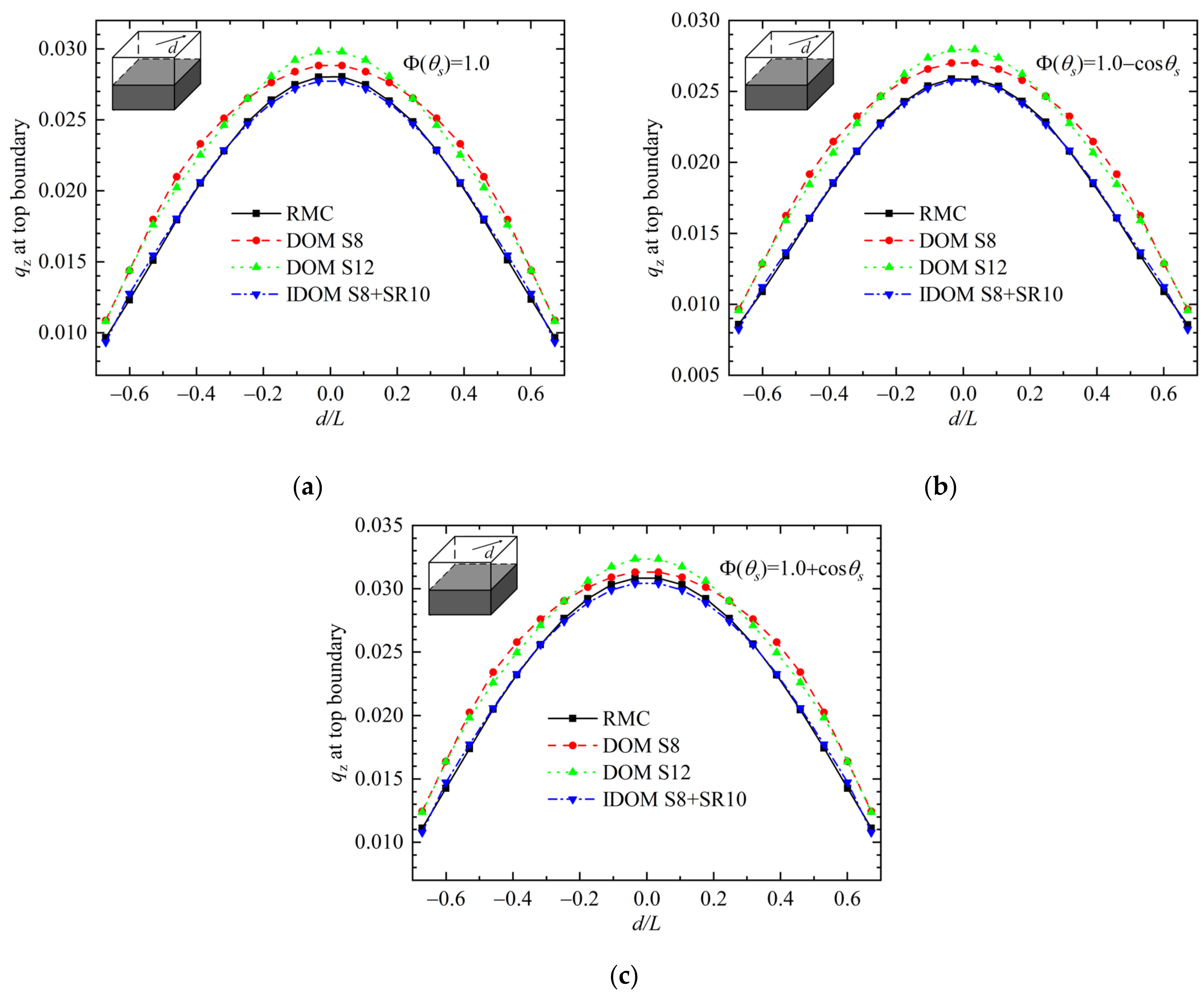
3.2. Ray Effects in IDOM

In this section, the IDOM and DOM are applied to calculate radiative heat flux distributions along the diagonal line of the top boundary for all three cases. Ray effects in both methods are investigated by considering the reverse Monte Carlo method with 2 million energy bundles as the benchmark solution. For all cases considered in this section, NX = 20 is applied to spatial discretization.

Figure 3 shows radiative heat flux along the diagonal line of the top boundary in Case 1. In this case, the enclosed medium is cold and purely scattering, and the optical thickness βL is 1.0. The bottom boundary is hot with unity emissive power, while the other boundaries are all cold. As shown in the figure, the difference between heat flux calculated by DOM S8 and RMC is obvious because of ray effects. Comparing with the RMC method, there is still obvious difference even a higher order scheme (DOM S12) is applied. Results calculated by IDOM are in better agreement with the benchmark solution. Take results in Figure 3b for example, the average errors of heat flux by DOM S8 and DOM S12 are about 18%, and the average errors for IDOM S8 + SR10 (M = 530) and S8 + SR20 (M = 2058) reduce to 4.3% and 2.0%, respectively. It shows that the IDOM can reduce ray effects effectively both in isotropic and anisotropic scattering medium.

Heat flux at the top boundary in Case 2 is displayed in Figure 4. In this case, the enclosed medium is absorbing and scattering with optical thickness βL equal to 2.0. The bottom half of the medium is hot with a unity emission, while the top half and all boundaries are cold. As displayed in the figure, both DOM S8 and DOM S12 suffer from obvious ray effects due to the non-uniform emission of the medium. Their calculation results are significantly larger than the benchmark solution, and the average errors are larger than 8.2%. In contrast, heat flux calculated by IDOM S8 + SR10 is in good agreement with the benchmark solution and the average error is less than 1.4%. The above results once again show that IDOM can effectively reduce the error of ray effects and significantly improve the accuracy of radiative heat flux.

Figure 5 shows heat flux along the diagonal line of the top boundary in Case 3. All the conditions are the same as those in Case 2, except that the medium has uniform emission in this case. As displayed in the figure, DOM with both S8 and S12 has the same and acceptable accuracy since ray effects is not obvious in the uniform medium. Obvious improvement of the IDOM results can still be observed and the heat flux curves by the IDOM confirm excellently with those of the RMC method. In DOM, the results keep unchanged while the angular discrete scheme changes from S8 to S12. This means the ray effects are not the cause of the error for DOM in this case, and false scattering may be the main reason and this will be investigated in the following section. Furthermore, as displayed in Figure 5d, results of both RMC and IDOM show that heat flux with forward scattering medium is smaller than that with backward scattering medium in the middle of the boundary, while is larger at the edge of the boundary. At first glance, the trend is contradictory to our initial expectation that the forward scattering medium benefits for energy transfer and should have larger radiative heat flux at the boundary. This interesting result, which is related to the effect of scattering phase function on radiative transfer, is to be studied in Section 3.4.

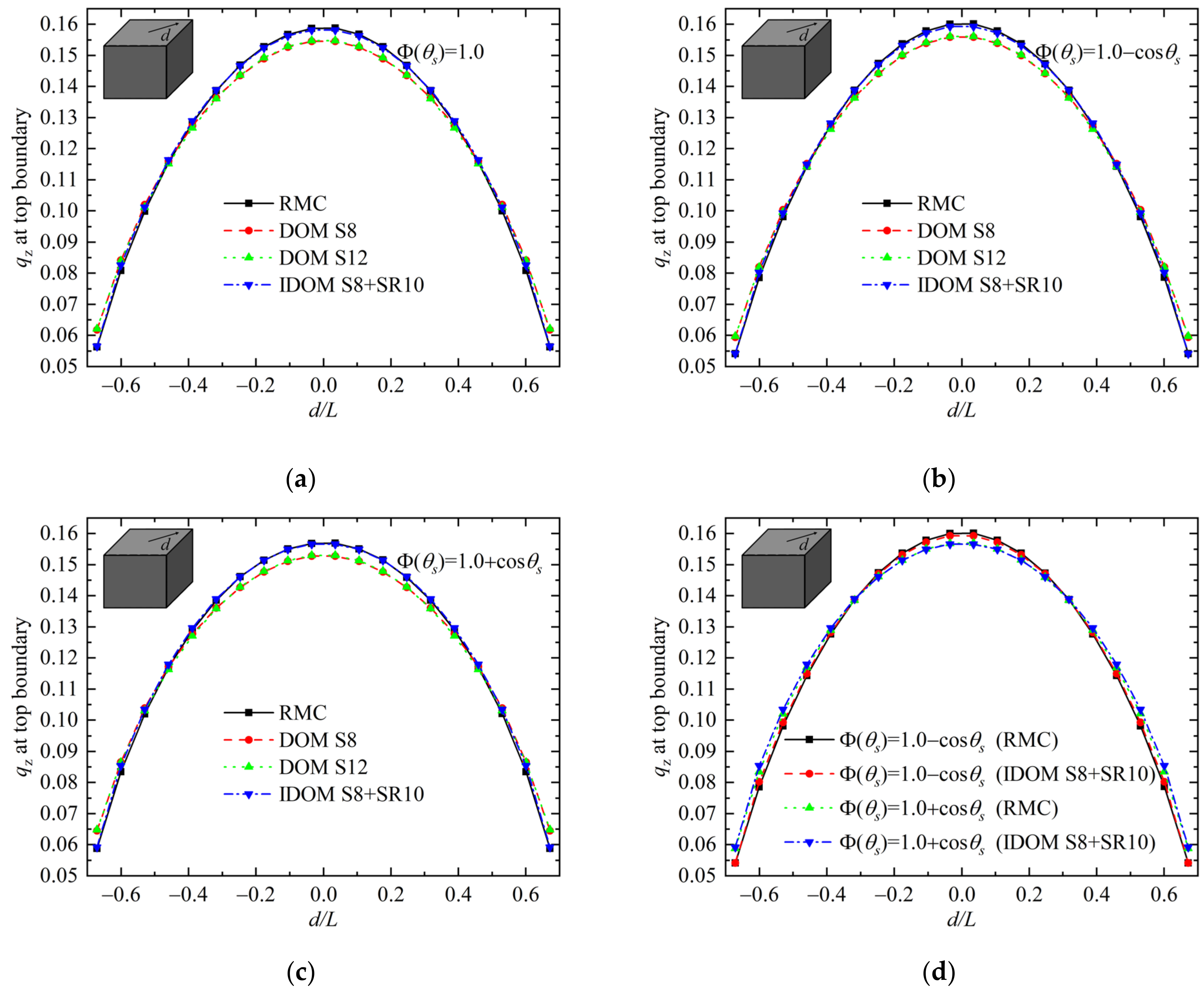
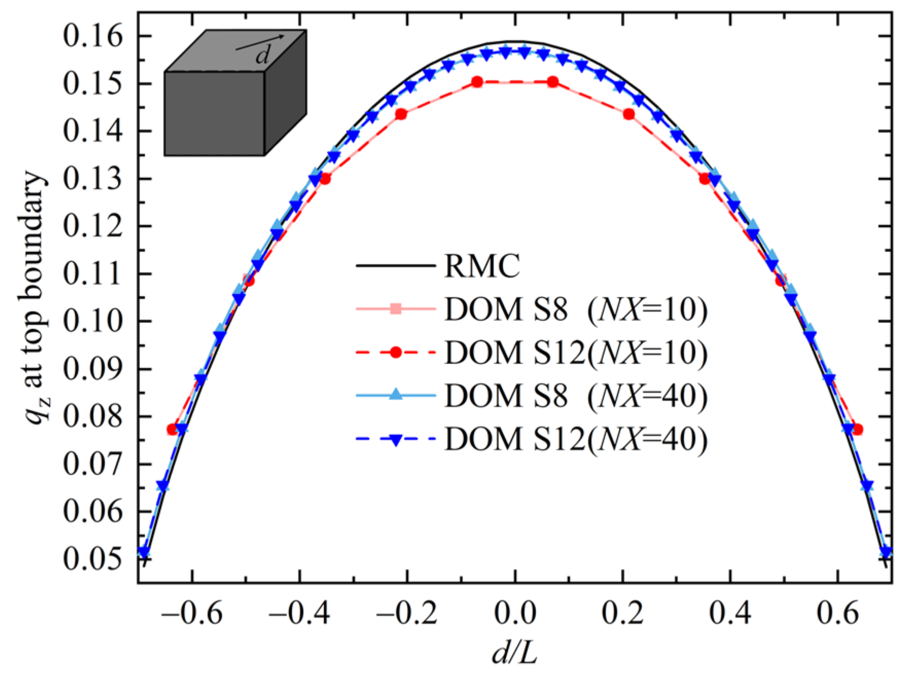
3.3. False Scattering in IDOM

As shown in previous section, the IDOM reduces ray effects effectively since radiative intensity in a large number of discrete directions are obtained and used to evaluate radiative heat flux. However, false scattering and ray effects usually have impacts on each other, reducing one of them may increase the other one [21,25,26]. Then, the false scattering in IDOM is to be examined in this section.

In order to decouple the errors caused by ray effects and false scattering on final results, Case 3 with uniform emission medium is considered in which ray effects is not obvious as shown in Figure 5. The enclosed medium is isotropic scattering, and the optical thickness βL is equal to 2.0. Heat flux along the diagonal line of the top boundary with different spatial discrete number NX = 10 and 40 are depicted in Figure 6. From the figure, results calculated by DOM S8 and DOM S12 agree well with each other for all the spatial discrete numbers, which shows ray effects has no influence on results accuracy in these cases. Meanwhile, as the number of NX increases, results of DOM have better accuracy. This means the false scattering is the main cause of the error, and this error is reduced by refining spatial grids.

Figure 7 shows radiative heat flux distribution at top boundary in Case 3 with different optical thicknesses. As shown in Figure 7a,b, when optical thickness is 1.0 and 2.0, heat flux by the IDOM is in good agreement with the benchmark solution and the average errors are only 0.83% and 0.79%, while the average errors of heat flux by DOM are 3.54% and 3.75%. These results show that the IDOM can significantly reduce false scattering error comparing with the conventional DOM.

When the optical thickness is thick, as shown in Figure 7c, although the IDOM has better accuracy than the DOM, it also suffers from false scattering with low spatial resolution (NX = 10). Refining the spatial resolution to NX = 20, the IDOM significantly reduces the false scattering error, and its calculation results are in good agreement with the benchmark solution, while the DOM still has obvious false scattering error, as shown in the Figure 7d. These results indicate that, if the radiative system studied has a thick optical thickness, it is also necessary to refine spatial grids in IDOM to reduce the false scattering error. Meanwhile, the false scattering error in IDOM is much less than that in the conventional DOM if the same spatial grids are employed.

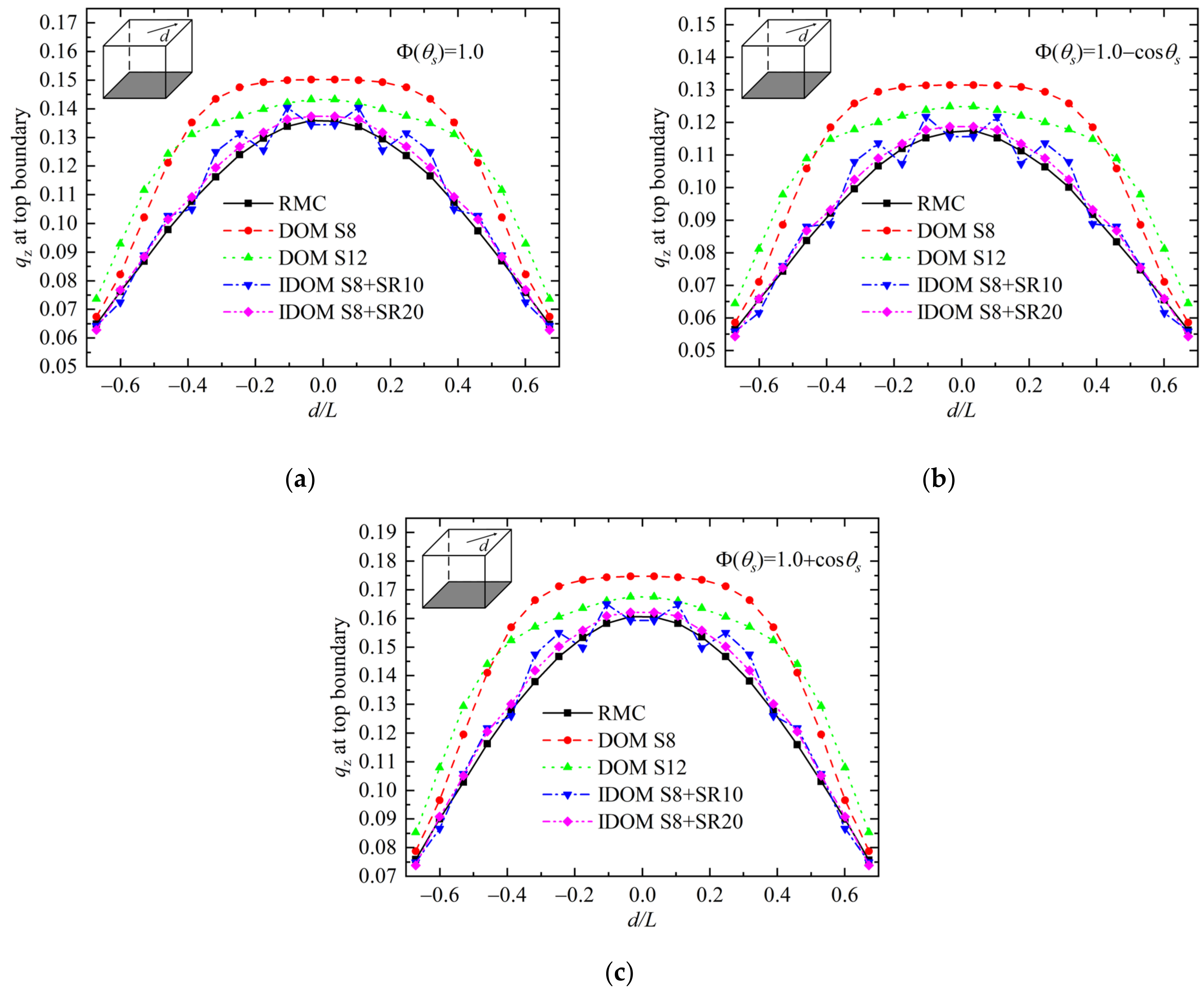
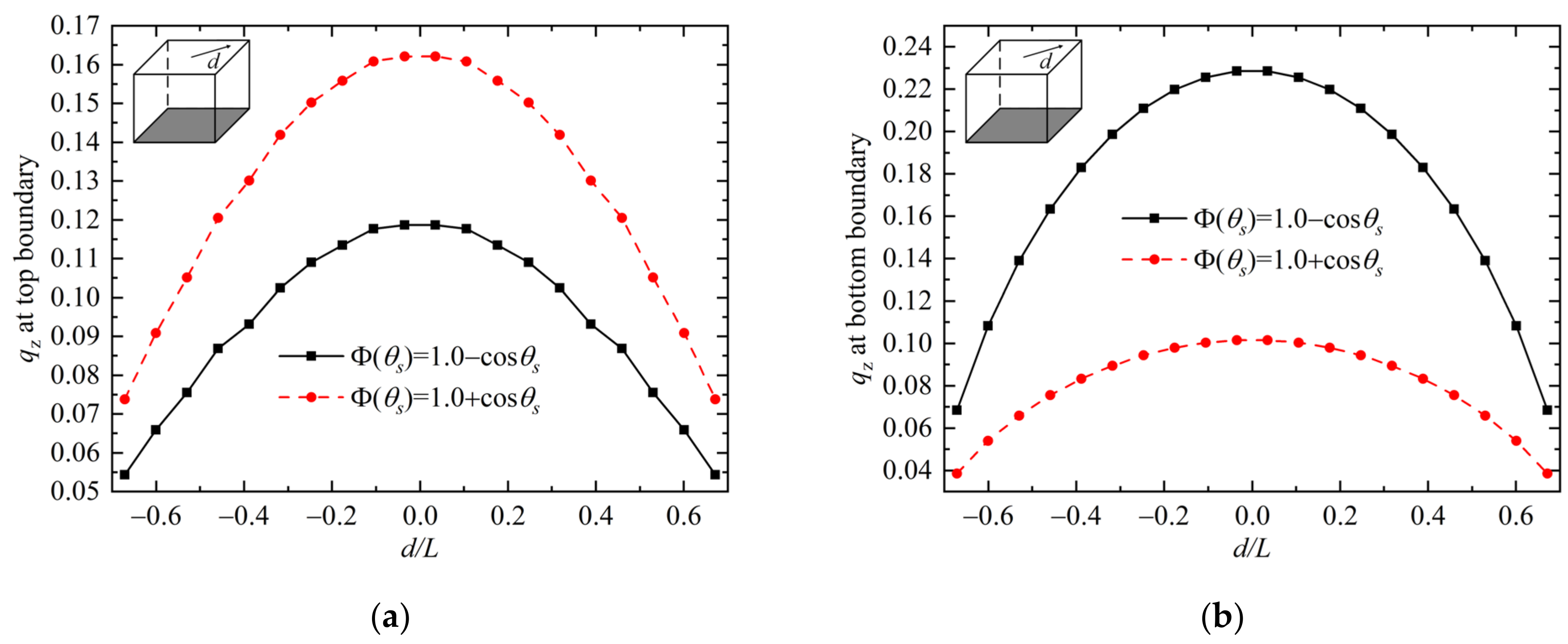
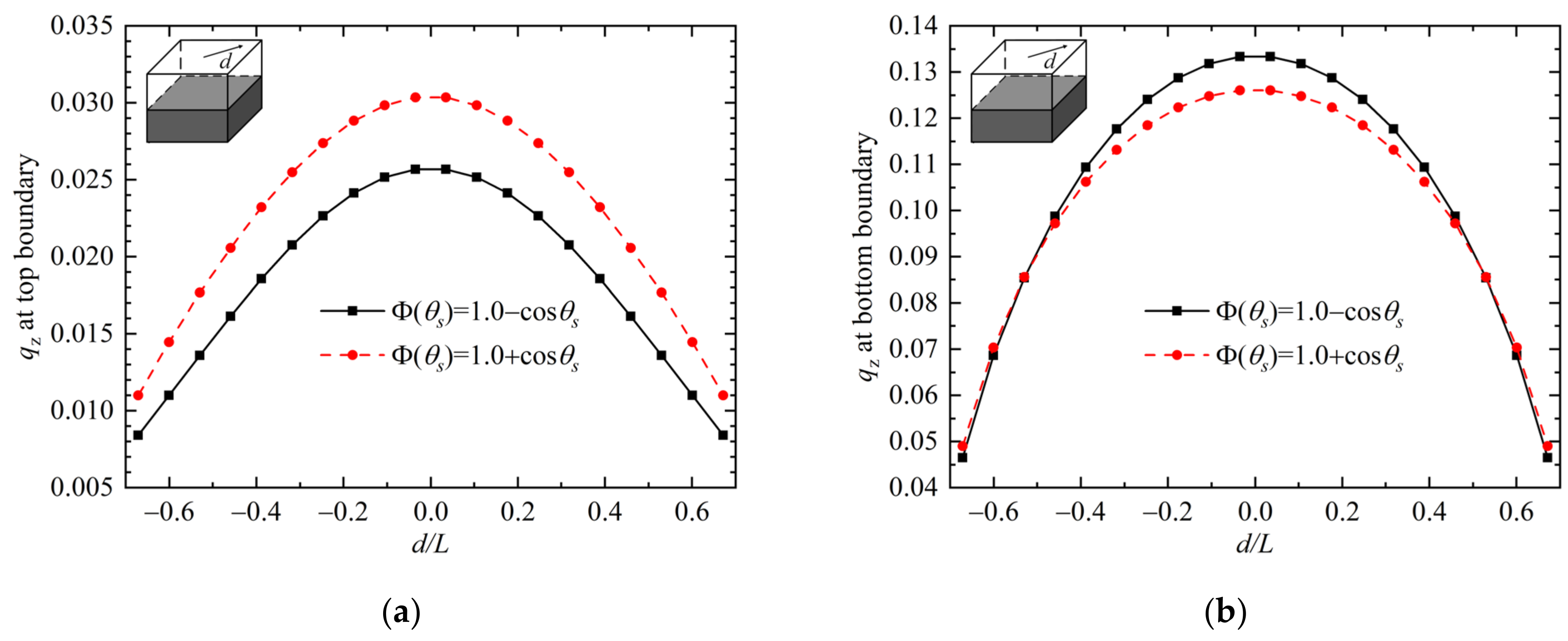
3.4. Effect of Scattering Phase Functions on Radiative Transfer

Scattering behavior is one of the key factors affecting radiative transfer. Radiative rays change their original propagating directions by scattering in the medium, and the directional distribution of scattered rays is described by the scattering phase function. In this section, the effect of scattering phase function on radiative energy transfer is analyzed by the IDOM. Radiative heat flux results calculated by IDOM S8 + SR20 with discrete number NX = 20, which have been shown to have good accuracy in Section 3.2, are compared for media with different scattering phase functions.

Figure 8 shows heat flux along the diagonal line on boundary of Case 1. As displayed in the figure, heat flux at the top boundary with forward scattering medium is larger than that with backward scattering medium, while the trend of heat flux at the bottom boundary influenced by scattering phase function is reverse. The explanation for these results is straightforward. The forward scattering medium scatters more radiative energy forward; thus, heat flux at boundaries located in the upward direction of emission plane (z = 0) has bigger values, and at boundaries located in the downward direction has smaller values.

Heat flux curves along the diagonal line at boundaries in Case 2 are presented in Figure 9. At the top boundary in Figure 9a, heat flux with forward scattering medium is larger than that with backward scattering medium, and this trend is the same as that in Case 1. However, at the bottom boundary in Figure 9b, heat flux at the center area with forward scattering medium is smaller than that with backward scattering medium, while an opposite trend is observed at the edge area. This is because radiative energy received by the bottom boundary is affected by both the backward scattering part (of the energy emitted upward by the source) and the forward scattering part (of the energy emitted downward by the source). These two parts are influenced by the scattering phase functions in an opposite way, and the trend of radiative heat flux at the bottom boundary depends on the overall effects of these two parts. If we revisit the results in Figure 5d, the same trend as in Figure 9b can be observed and can be explained similarly. These results show that unlike the case with emitting boundary, the effect of scattering phase functions on radiative transfer within systems with emitting medium is complicated and needs to be considered case by case.

3.5. Computation Cost Comparison

For conventional DOM, its computation time mainly depends on the number of control volumes, discrete directions, and the number of iterations. Take the cubic radiative system in Figure 2 for example, assuming that the number of control volumes is N_s³, the number of discrete directions is N and the number of iterations is N_i, the computation time of the conventional DOM is roughly proportional to N_s³ × N² × N_i. For IDOM, in addition to the computation time spent in the first step, which is the same as that of the conventional time, extra computation time to make the integral calculation of Equation (13) in the second step is needed. On average, the number of integrated control volumes in each direction is around N_s. Assuming the number of new discrete directions is M and heat flux at N_q points is to be calculated, the additional computation time of IDOM is roughly proportional to N_s × M × N × N_q. Since N_s × M × N × N_q is much smaller than N_s³ × N² × N_i in most cases, the additional computation time of IDOM is almost negligible compared with the computation time of the conventional DOM.

The above analysis can also be proved by calculation times of different methods listed in

Table 2. Calculation times consumed by different methods, sec.

Cases	A1	RMC	DOM S8	DOM S12	IDOM S8 + SR10	IDOM S8 + SR20
Case 1	0	41.64	1.22	5.88	1.30	1.53
	−1	42.91	1.77	7.64	1.86	2.03
	1	41.86	1.53	6.61	1.63	1.78
Case 2	0	37.70	1.78	8.27	1.92	2.13
	−1	38.83	2.61	11.34	2.64	2.88
	1	38.05	2.23	9.83	2.27	2.52
Case 3	0	42.48	1.98	8.47	2.03	2.20
	−1	43.30	2.78	12.13	2.84	3.02
	1	42.69	2.30	9.89	2.33	2.53

. The computation time is about specific cases considered in Section 3.2. Take Case 1 with isotropic scattering medium as listed in the first line of the table for instance, calculation time consumed by DOM increases from 1.22 s to 5.88 s with angular discretization number increases from 80 (S8) to 168 (S12), while the average errors of heat flux by DOM S8 and DOM S12 are about 16% as shown in Figure 3a. For IDOM S8 + SR10, its calculation time is only about 0.08 s more than that of DOM S8, while the average error of heat flux reduces to about 3.8%. This error in IDOM can be further reduced by using more new directions (such as IDOM S8 + SR20) with negligible increased computation time. There are similar conclusions in the other cases. That is to say, IDOM can provide results with much higher accuracy while keeping computation time almost the same as the conventional DOM.

Furthermore, since the second step in IDOM is merely an integral calculation, the memory usage for new variables in IDOM is limited and negligible compared with that of the conventional DOM.

4. Conclusions

The IDOM is extended to calculate radiative heat flux in three-dimensional radiative systems with anisotropic scattering medium. Radiative heat flux calculated in IDOM is divided into the direct part contributed by emission of the media and the boundaries and the indirect part contributed by in-scattering of the media and reflection of the boundaries. Theoretical analysis indicates that IDOM has higher accuracy than the conventional DOM.

Ray effects, together with false scattering in IDOM, were investigated in this paper by considering the reverse Monte Carlo method as the benchmark solution. In the considered radiative system with only one boundary emission, which suffers obvious ray effects, the average error of heat flux was about 16%, and the calculation time was about 1.22 s for conventional DOM. For IDOM, the average error of heat flux was less than 4% and the calculation time was only 0.08 s more than that of the conventional DOM. More numerical experiments show that the IDOM could reduce ray effects effectively both in isotropic and anisotropic scattering medium with negligible increased computation time compared with the conventional DOM. Meanwhile, in a radiative system with uniform medium emission of which the accuracy is not influenced by ray effects, the calculation error of conventional DOM was larger than 3% while that of IDOM is less than 1%, when the same spatial resolution was applied in both methods. This numerical experiment proves that the false scattering error in IDOM was much smaller than that in the conventional DOM. In a word, the IDOM can overcome the shortages of the conventional DOM well, while inheriting its advantages such as high computation efficiency and easy implementation.

The IDOM was also applied to investigate the effect of scattering phase functions on radiative transfer. Results show that the trend of radiative heat flux with different scattering phase functions is simple for cases of emitting boundaries, while it is complicated for cases of emitting media.

References

1. Howell, J.R.; Siegel, R.; Mengüç, M.P. Thermal Radiation Heat Transfer, 5th ed.; CRC Press: Boca Raton, FL, USA, 2011. [Google Scholar]
2. Modest, M.F. Radiative Heat Transfer, 3rd ed.; Academic Press: San Diego, CA, USA, 2013. [Google Scholar]
3. Chai, J.C.; Lee, H.S.; Patankar, S.V. Ray effect and false scattering in the discrete ordinates method. Numer. Heat Transf. Part B Fundam. 1993, 24, 373–389. [Google Scholar] [CrossRef]
4. Tan, H.-P.; Zhang, H.-C.; Zhen, B. Estimation of ray effect and false scattering in approximate solution method for thermal radiative transfer equation. Numer. Heat Transf. Part A Appl. 2004, 46, 807–829. [Google Scholar] [CrossRef]
5. Hunter, B.; Guo, Z. Numerical smearing, ray effect, and angular false scattering in radiation transfer computation. Int. J. Heat Mass Transf. 2015, 81, 63–74. [Google Scholar] [CrossRef]
6. Liu, F.; Becker, H.A.; Pollard, A. Spatial differencing schemes of the discrete-ordinates method. Numer. Heat Transf. Part B Fundam. 1996, 30, 23–43. [Google Scholar] [CrossRef]
7. Jessee, J.P.; Fiveland, W.A. Bounded, High-Resolution Differencing Schemes Applied to the Discrete Ordinates Method. J. Thermophys. Heat Transf. 1997, 11, 540–548. [Google Scholar] [CrossRef]
8. Coelho, P.J. Bounded Skew High-Order Resolution Schemes for the Discrete Ordinates Method. J. Comput. Phys. 2002, 175, 412–437. [Google Scholar] [CrossRef]
9. Li, H.-S.; Gilles, F. Reduction of False Scattering of the Discrete Ordinates Method. J. Heat Transf. 2002, 124, 837–844. [Google Scholar] [CrossRef]
10. Li, H.-S. Reduction of false scattering in arbitrarily specified discrete directions of the discrete ordinates method. J. Quant. Spectrosc. Radiat. Transf. 2004, 86, 215–222. [Google Scholar] [CrossRef]
11. Li, H.-S.; Flamant, G.; Lu, J.-D. Mitigation of ray effects in the discrete ordinates method. Numer. Heat Transf. Part B Fundam. 2003, 43, 445–466. [Google Scholar] [CrossRef]
12. Tencer, J. Ray Effect Mitigation through Reference Frame Rotation. J. Heat Transf. 2016, 138, 112701. [Google Scholar] [CrossRef]
13. Camminady, T.; Frank, M.; Küpper, K.; Kusch, J. Ray effect mitigation for the discrete ordinates method through quadrature rotation. J. Comput. Phys. 2019, 382, 105–123. [Google Scholar] [CrossRef] [Green Version]
14. Zhang, B.; Zhang, L.; Liu, C.; Chen, Y. Goal-Oriented Regional Angular Adaptive Algorithm for the SN Equations. Nucl. Sci. Eng. 2018, 189, 120–134. [Google Scholar] [CrossRef]
15. Dargaville, S.; Smedley-Stevenson, R.P.; Smith, P.N.; Pain, C.C. Goal-based angular adaptivity for Boltzmann transport in the presence of ray-effects. J. Comput. Phys. 2020, 421, 109759. [Google Scholar] [CrossRef]
16. Lathrop, K.D. Remedies for Ray Effects. Nucl. Sci. Eng. 1971, 45, 255–268. [Google Scholar] [CrossRef]
17. Morel, J.E.; Wareing, T.A.; Lowrie, R.B.; Parsons, D.K. Analysis of Ray-Effect Mitigation Techniques. Nucl. Sci. Eng. 2003, 144, 1–22. [Google Scholar] [CrossRef]
18. Frank, M.; Kusch, J.; Camminady, T.; Hauck, C.D. Ray Effect Mitigation for the Discrete Ordinates Method Using Artificial Scattering. Nucl. Sci. Eng. 2020, 194, 971–988. [Google Scholar] [CrossRef] [Green Version]
19. Ramankutty, M.A.; Crosbie, A.L. Modified discrete ordinates solution of radiative transfer in two-dimensional rectangular enclosures. J. Quant. Spectrosc. Radiat. Transf. 1997, 57, 107–140. [Google Scholar] [CrossRef]
20. Ramankutty, M.A.; Crosbie, A.L. Modified discrete-ordinates solution of radiative transfer in three-dimensional rectangular enclosures. J. Quant. Spectrosc. Radiat. Transf. 1998, 60, 103–134. [Google Scholar]
21. Coelho, P.J. The role of ray effects and false scattering on the accuracy of the standard and modified discrete ordinates methods. J. Quant. Spectrosc. Radiat. Transf. 2002, 73, 231–238. [Google Scholar] [CrossRef]
22. Tan, Z.-M.; Hsu, P.-F.; Wu, S.-H.; Wu, C.-Y. Modified YIX Method and Pseudoadaptive Angular Quadrature for Ray Effects Mitigation. J. Thermophys. Heat Transf. 2000, 14, 289–296. [Google Scholar] [CrossRef]
23. Huang, Z.-F.; Zhou, H.-C.; Hsu, P.-f. Improved Discrete Ordinates Method for Ray Effects Mitigation. J. Heat Transf. 2011, 133, 044502. [Google Scholar] [CrossRef]
24. Li, H.-S.; Zhou, H.-C.; Lu, J.-D.; Zheng, C.-G. Computation of 2-D pinhole image-formation process of large-scale furnaces using the discrete ordinates method. J. Quant. Spectrosc. Radiat. Transf. 2003, 78, 437–453. [Google Scholar] [CrossRef]
25. Raithby, G.D. Evaluation of discretization errors in finite-volume radiant heat transfer predictions. Numer. Heat Transf. Part B Fundam. 1999, 36, 241–264. [Google Scholar] [CrossRef]
26. Coelho, P.J. Advances in the discrete ordinates and finite volume methods for the solution of radiative heat transfer problems in participating media. J. Quant. Spectrosc. Radiat. Transf. 2014, 145, 121–146. [Google Scholar] [CrossRef]
27. Lu, X.; Hsu, P.F. Parallel computing of an integral formulation of transient radiation transport. J. Thermophys. Heat Transf. 2003, 17, 425–433. [Google Scholar] [CrossRef]
Figure 1. A control volume in three-dimensional radiative systems.
Energies 14 06839 g001
Figure 2. Calculation model for radiative intensity in a new direction in IDOM.
Energies 14 06839 g002
Figure 3. Heat flux at the boundary of Case 1: (a) results for A1 = 0; (b) results for A1 = −1; (c) results for A1 = 1.
Energies 14 06839 g003
Figure 4. Heat flux at the boundary of Case 2: (a) results for A1 = 0; (b) results for A1 = −1; (c) results for A1 = 1.
Energies 14 06839 g004
Figure 5. Heat flux at the boundary of Case 3: (a) results for A1 = 0; (b) results for A1 = −1; (c) results for A1 = 1; (d) results comparison for A1 = −1 and 1.
Energies 14 06839 g005
Figure 6. Heat flux by DOM with different angular and spatial discretization of Case 3.
Energies 14 06839 g006
Figure 7. Heat flux of Case 3 with different optical thicknesses (a) βL = 1.0 and NX = 10; (b) βL = 2.0 and NX = 10; (c) βL = 10.0 and NX = 10; (d) βL = 10.0 and NX = 20.
Energies 14 06839 g007
Figure 8. Heat flux with different scattering phase functions in Case 1: (a) results at top boundary; (b) results at bottom boundary.
Energies 14 06839 g008
Figure 9. Heat flux with different scattering phase functions in Case 2: (a) results at top boundary; (b) results at bottom boundary.
Energies 14 06839 g009