Forecasting the CO₂ Emissions at the Global Level: A Multilayer Artificial Neural Network Modelling

Abstract

Better accuracy in short-term forecasting is required for intermediate planning for the national target to reduce CO₂ emissions. High stake climate change conventions need accurate predictions of the future emission growth path of the participating countries to make informed decisions. The current study forecasts the CO₂ emissions of the 17 key emitting countries. Unlike previous studies where linear statistical modeling is used to forecast the emissions, we develop a multilayer artificial neural network model to forecast the emissions. This model is a dynamic nonlinear model that helps to obtain optimal weights for the predictors with a high level of prediction accuracy. The model uses the gross domestic product (GDP), urban population ratio, and trade openness, as predictors for CO₂ emissions. We observe an average of 96% prediction accuracy among the 17 countries which is much higher than the accuracy of the previous models. Using the optimal weights and available input data the forecasting of CO₂ emissions is undertaken. The results show that high emitting countries, such as China, India, Iran, Indonesia, and Saudi Arabia are expected to increase their emissions in the near future. Currently, low emitting countries, such as Brazil, South Africa, Turkey, and South Korea will also tread on a high emission growth path. On the other hand, the USA, Japan, UK, France, Italy, Australia, and Canada will continuously reduce their emissions. These findings will help the countries to engage in climate mitigation and adaptation negotiations.

1. Introduction

There is wide consensus among scientists and policymakers that global warming as defined by the Intergovernmental Panel on Climate Change (IPCC) should be pegged at 1.5° Celsius above the pre-industrial level of warming in order to maintain environmental sustainability [1]. The threats and risks of climate change have been evident in the form of various extreme climate events, such as tsunamis, glacier melting, rising sea levels, and heating up of the atmospheric temperature. Emissions of greenhouse gases, such as carbon dioxide (CO₂) are the main cause of global warming. The Kyoto protocol and the subsequent Paris climate summit have urged the global North and South to cooperate and bear the responsibility of reducing the CO₂ emissions together on a partnership basis. However, climate politics is often not in sync with all the agreements of the Paris climate deals. Especially, since the United States (US) is not a signatory to the Paris climate accords, the international cooperation sought between the industrialized and industrializing countries is slow. Given this broad context of looming climate change threats and the slow pace of actions on reducing CO₂ emissions by the countries, more scientific research must be undertaken to understand the exact nature of the threats. Knowing the level of CO₂ emissions by the high emitting countries in near future will provide actionable insights on climate policy. Such information will aid in fostering the cooperation talks in the upcoming United Nations (UN) COP26 climate conference from 31 October–12 November 2021 in Glasgow, United Kingdom (UK).

Estimating CO₂ has often been done in the context of a school of thought in research, popularly known as the environmental Kuznets curve (EKC) hypothesis. This hypothesis states that environmental degradation, such as air pollution (CO₂, SO₂, NO₂, and SPM emissions), water pollution, and solid waste generation follow an inverted-U relationship with economic growth [2,3]. During the initial level of a country’s economic growth, the environmental pollution increases due to rapid expansion in economic activities, however after a threshold level of income per capita in the country is reached, the environmental quality improves because of a higher share of public funds being devoted to improving the environmental quality [4,5,6]. Despite the last three decades of empirical research in an attempt to estimate the turning point of this EKC, there has still not been consensus about a global turning point. However, there has been tremendous growth in terms of methodological sophistication to estimate both time-series and panel data available for various environmental pollutants and countries [7,8,9,10,11,12].

A detailed literature review has been undertaken covering the most recent published papers to present the state-of-the-art advancements in EKC studies. Most of these studies have highlighted the role of renewable energy in reducing CO₂ emissions. Dong et al. [13] examined the dynamic causal links among per capita carbon dioxide (CO₂) emissions, per capita GDP, per capita fossil fuels consumption, per capita nuclear energy consumption, and per capita renewable energy consumption for China. They found that both nuclear energy and renewable energy play important roles in mitigating CO₂ emissions in both the short and long run, while fossil fuels consumption is indeed the dominant reason for promoting CO₂ emissions. They observed that renewable energy has a higher CO₂ mitigating effect than nuclear power. Kim and Park [14] from a study of 30 countries for a period of 2000–2013, suggested that a developed financial market in a country helps deploy more renewable energy and, in turn, can reduce CO₂ emissions. Paramati et al. [15] from panel data of G20 countries show that foreign direct investment (FDI) inflows significantly reduces CO₂ emissions in both developed and developing economies while stock market growth reduces in developed economies. They also found that renewable energy consumption substantially reduces CO₂ emissions and increases economic output across the countries in their panels.

In a study, Li et al. [16] used the data from China and Nigeria from 1991–2014 to derive the energy efficiency measures in the mining and extractive related sectors. Using several econometric time series methods, they concluded that energy efficiency in the mining and extractive-related sector and the circular economy have not translated into CO₂ emission reduction in both countries. However, economic growth, energy use (non-renewable energy), and clean energy substitution (renewable energy) are essential factors in mitigating CO₂ emissions. Lorente et al. [17] employed a carbon emission function to investigate the relationship between economic growth and CO₂ emissions in five European Union countries, namely, Germany, France, Italy, Spain, and the United Kingdom, for the 1985–2016 period. They found an N-shaped relationship between economic growth and CO₂ emissions in the EU-5 countries. Further, they observed that renewable electricity consumption, natural resources, and energy innovation improve environmental quality. Using a panel of 20 organisations for economic co-operation and development (OECD) nations for the period, 1870 to 2014, Churchill et al. [18] found support for the EKC hypothesis for the panel as a whole with turning points in income per capita that lie between $18,955 and $89,540 (in 1990 US$).

A study by Chen et al. [19] used the Chinese data for the period 1980–2014 and explored the relationships among per capita CO₂ emissions, GDP, renewable and non-renewable energy production, and foreign trade. They found that there is a long-run relationship among those variables. They also found that China does not follow the EKC for CO₂ emissions under the influence of economic growth, non-renewable energy production, and foreign trade. However, the addition of renewable energy production variables supported the U-shaped EKC hypothesis in the long run.

Using data for 1995–2018, pooled mean group-autoregressive distributed Lag (PMG-ARDL) estimator, and heterogeneous causality tests, Gyamfi et al. [20] failed to confirm an N-shaped EKC in the emerging seven, rather they confirm the existence of an inverted U-shaped EKC in the study countries. They suggested the increased use of renewable energy to mitigate pollutant emissions in these countries. Using the data from a study of BRICS economies for the period of 1980 to 2016, Khattak et al. [21] investigated the complex interaction between innovation, renewable energy consumption, and CO₂ emissions, under the EKC framework. They found that innovation activities have failed to disrupt CO₂ emission in China, India, Russia, and South Africa, except for Brazil. They also showed that renewable energy consumption has mitigated CO₂ emission in the BRICS panel, Russia, India, and China but not in South Africa. Further, except for India and South Africa, they observed the EKC hypothesis in all the BRICS economies. Employing a stochastic impacts by regression on population, affluence, and technology (STIRPAT) framework to the data for the period of 1990–2017 from West Asia and Middle East nations, Kihombo et al. [22] probed the effects of technological innovation, financial development (FD), and economic growth (GDP) on the ecological footprint (EF) controlling for urbanization. They observed that a 1% upsurge in technological innovation decreases EF by 0.01%. However, a 1% rise in FD boosts the level of EF by 0.0016%, inferring that FD stimulates ecological degradation. They also showed the EKC hypothesis in the selected countries.

In India’s case, using data for a period of 1990–2015 and several time series econometric models, Kirikkaleli and Adebayo [23] found a long-run cointegration relationship between consumption-based carbon dioxide emissions and its possible determinants. They also found that public-private partnership investment in energy makes a positive contribution to consumption-based carbon dioxide emissions in the long run. Further, public-private partnership investment in energy and renewable energy consumption also significantly causes consumption-based carbon dioxide emissions at different frequency levels in the country. Using annual data from six South Asian economies for a period of 1980–2016 and autoregressive distributed lag (ARDL) regression, Murshed [24] examined the validity of the greenhouse emissions-induced EKC hypothesis, controlling for liquefied petroleum gas (LPG) consumption, FDI inflows, and trade openness. The analysis confirms the authenticity of the EKC hypothesis for Bangladesh, India, Sri Lanka, and Bhutan. They suggested fuel-diversification policies for the government’s of these countries. Using the data for a period of 1995–2017 from 34 high-income countries from three continents (Asia, Europe, and America), Khan et al. [25] explained the nexus of GHG emission with tourism, financial development index, energy use, renewable energy, and trade. They observed a country-level reciprocal connection of GHG with financial development in 11 countries, renewable energy in 22 countries, trade openness in five countries, and tourism in 12 countries. Using two-panel data sets of 17 major developing and developed countries as well as six geo-economic regions of the world during 1990–2014, Yao et al. [26] examined the dynamic relationship between renewable energy consumption rate (RER) and the EKC hypothesis. Using several econometric methods, they verified both the EKC and renewable energy Kuznets Curve (RKC) hypotheses, indicating that a 10% rise in RER would lead to a 1.6% carbon emission reduction. Saleem et al. [27] used the data for a period of 1980–2015 from selected Asian countries and employing several econometrics models, found the presence of an EKC hypothesis, where the impact of GDP growth and the square of GDP growth on CO₂ emissions are positive and negative, respectively. They also found that lower-income economies do not support the EKC hypothesis.

Employing the second-generation panel cointegration methodologies and data for 1984–2016, Ahmad et al. [28] analyzed the linkages between natural resources, technological innovations, economic growth, and the resulting ecological footprint in emerging economies. They observed the existence of slope heterogeneity across countries and correlation amongst cross-sectional units. They also found a stable, long-run relationship between the ecological footprint, natural resources, technological innovations, and economic growth. Another study in India by Usman et al. [29] studied the role of energy consumption and democratic regimes in the environmental degradation function for a period of 1971–2014. Using different time series econometric models, they confirmed the EKC hypothesis and divulged that energy consumption increases environmental degradation both in the long and short run. They suggested prioritizing energy conservation policy to mitigate environmental degradation and spur economic growth. Using data from 25 manufacturing subsectors in 38 countries from 2000 to 2014 and using an endogenous finite mixture model, Yang et al. [30] probed the effect of renewable energy in the EKC relationship. They found that with the growing impact of renewable energy consumption, nearly half of the sample countries and two-thirds of the subsectors have experienced the transformation of the nexus between manufacturing growth and emissions. Bilgili et al. [31] employed the panel quantile regression technique on a dataset from thirteen developed countries over the period 2003–2018 to find an inverted U-shaped nexus between economic growth and carbon emissions only in higher carbon-emitting countries, thus, confirming the EKC hypothesis. However, the U-shaped nexus is more predominant in lower carbon-emitting countries. They also found that energy efficiency research and development is more effective in curbing carbon emissions than fossil fuels and renewable energy research and development.

The literature review shows that significant advancement has taken place in the study of EKC in terms of the methods used. In particular, the dynamic time-series and panel cointegration models with the use of structural breaks have produced credible evidence. However, these dynamic time-series models used mostly the lag length to make the model dynamic and estimate the long-run relationship. Moreover, the time series or panel data estimations produce a single estimated parameter for the relationship within the whole sample period. The long-run relationship between CO₂ emissions and its predictors, such as GDP per capita, renewable energy consumption, and trade openness may not have been linear as the previous studies with statistical methods had tried to estimate. A few of the studies used the structural breaks to account for the major shifts in the environmental regulations and policies that may have affected the long-run relationship, but they finally showed constant estimates in observing the effect of GDP on environmental degradation for the whole time period. If the apparent nonlinearities existing in this relationship over a period of time are considered explicitly, more accurate predictions can be made, which has been done in the current study.

The current study aims to forecast the level of CO₂ emissions for 2017–2019 at the global level. CO₂ emission is the key contributor to climate change and there is a global consensus that the mean global surface temperature must be contained at 1.5 degrees C above the pre-industrial level. Consequently, several countries have signed the Paris agreement to reduce emissions within their national boundaries. Against this backdrop, it is essential to forecast the CO₂ emissions levels in the countries that emit a higher share. Such forecasting will help the national governments to adjust their climate policies.

Forecasting of CO₂ emissions at business as usual (BAU) scenario is a necessary tool for major greenhouse gas emitting countries for two main reasons. First, the global circulation models that are used to assess the physical impacts from climate change needs emissions as inputs. Since the countries included in this study are responsible for 79% of global emissions, forecasts of their emission level in the short run will be essential to gauge the impacts of climate change at the global level. Second, the responsibility to reduce CO₂ emissions as agreed at the Paris climate convention is proportional to the BAU levels of emissions. Hence, accurate prediction of emissions will put the right value of resources that these countries need to commit for the reduction of emissions. Since there is a trade-off between emission reduction and economic growth, these countries will be anxious that their emission levels are not underpredicted. Some of the countries may withdraw from a multilateral climate treaty if they find that they are at an economic disadvantage due to their pledge to reduce emissions. Accurate prediction of the BAU emission levels holds significance for a feasible action plan by the countries to reduce the global CO₂ emissions.

Considering that there might be a nonlinear relationship between the indicators of economic growth and the CO₂ emissions, we develop a multilayer artificial neural network (MLANN) model. A multilayer artificial neural network model is more efficient in capturing the nonlinearity present in the time series data and provides higher accuracy in forecasting the CO₂ emissions based on the past values of the emissions and the economic indicators, such as GDP, population density, and urbanization. Such forecasts for the near future will provide insights into regulations on pollution control.

The contributions of the paper are:

(i)

Formulation of CO₂ emissions prediction as an optimization problem.

(ii)

Development and performance evaluation of MLANN based model for prediction of CO₂ emissions.

(iii)

Forecasting of the missing CO₂ emission values for the years 2017–2019.

(iv)

Analysis of the results and their economic impact.

The rest of the paper is organized as follows. Materials and methods are discussed in Section 2. Section 3 deals with the development of a CO₂ prediction model using MLANN. Details of the simulation study are given in Section 4. It also contains data collection and preprocessing, training and testing of the model. Section 5 presents results and discussion. Finally, conclusion of the paper is presented in Section 6.

2. Materials and Methods

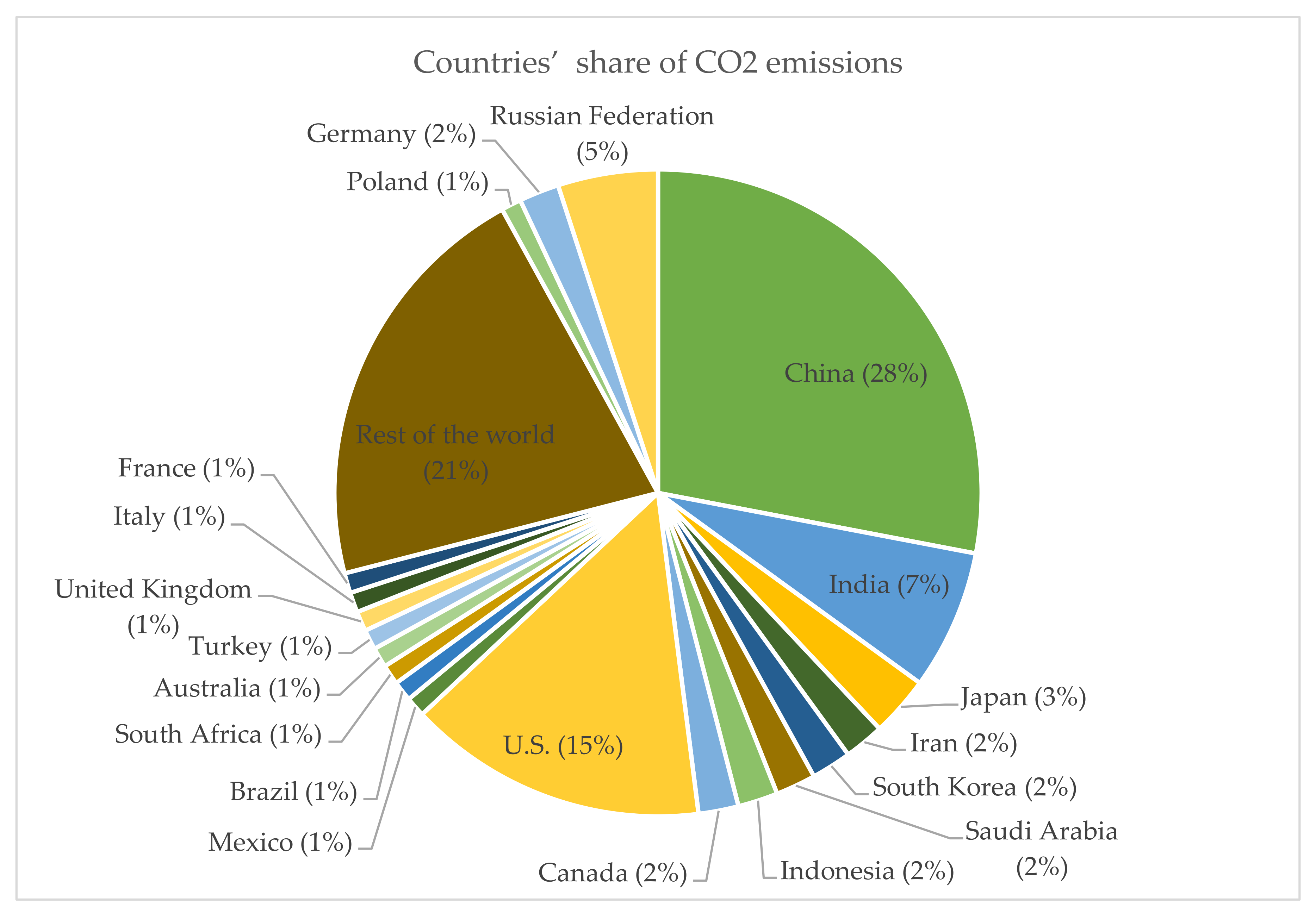
We have considered two types of countries—first, countries that emit 2% or more share of global CO₂ emissions and countries that emit less than 2% share. The selection of countries in this study is based on the data compiled by the International Energy Agency (IEA), which estimates carbon dioxide (CO₂) emissions from the combustion of coal, natural gas, oil, and other fuels, including industrial waste and non-renewable municipal waste. The specific data used are reproduced from the website Each Country’s Share of CO₂ Emissions | Union of Concerned Scientists (ucsusa.org) and are given below in Figure 1.

Table 1. High and Low emission countries.

Sl. No.	Group 1 High Emission Countries (with ≥2% Share)	Group 2 Low Emission Countries (with 1% Share)
1	China (28%)	Brazil (1%)
2	U.S. (15%)	South Africa (1%)
3	India (7%)	Mexico (1%)
4	Japan (3%)	Turkey (1%)
5	Iran (2%)	Australia (1%)
6	South Korea (2%)	United Kingdom (1%)
7	Saudi Arabia (2%)	Italy (1%)
8	Indonesia (2%)	France (1%)
9	Canada (2%)

describes the countries considered in this study under two groups—high emission and low emission countries.

The data on the output parameter, i.e., CO₂ emissions and the input parameters, such as GDP in constant US$ measured in 2011, trade as a percentage of GDP, and urban population for all the countries are drawn from the World Bank database. The period of the study is 1960 to 2016. The forecasting period is 2017, 2018, and 2019.

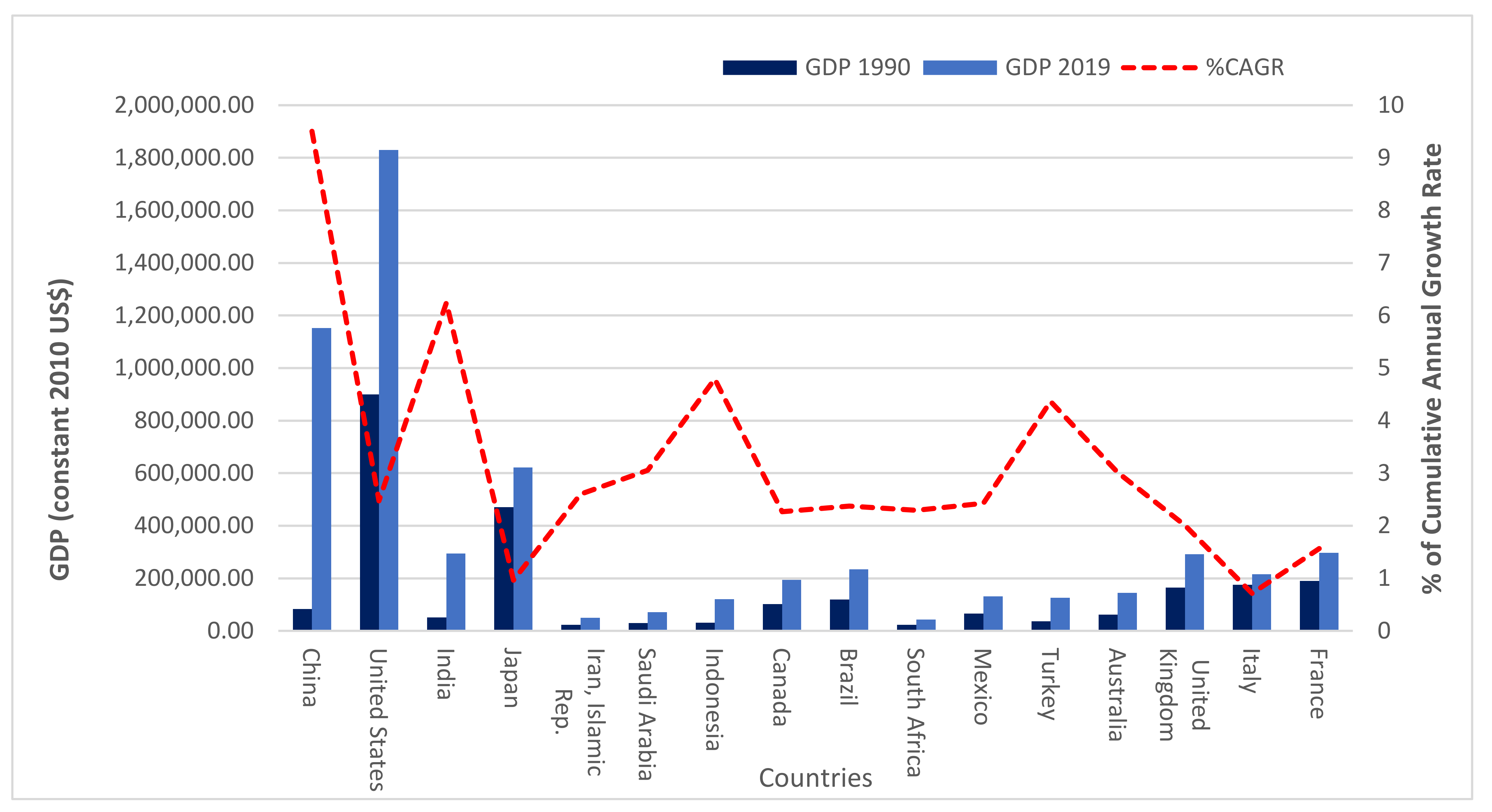
Figure 2 shows the GDP (constant in 2010 US$) for the countries considered in this study, in 1990 and 2016. Although the period of study is from 1960 to 2016, we chose the more recent years to compare the growth of the GDP. The countries shown in the X-axis are ordered from the highest emission status to the lowest among the 17 countries. The Y-axis shows the cumulative annual growth rate (CAGR) between 1990 and 2016. The countries showing a high growth rate in GDP are expectedly China with a CAGR of 9.5%, India with 6.2%, Indonesia with 4.8%, and Turkey with 4.4%. the countries that experienced low growth rates are Italy with 0.7%, Japan with 0.96%, and France with 1.56%.

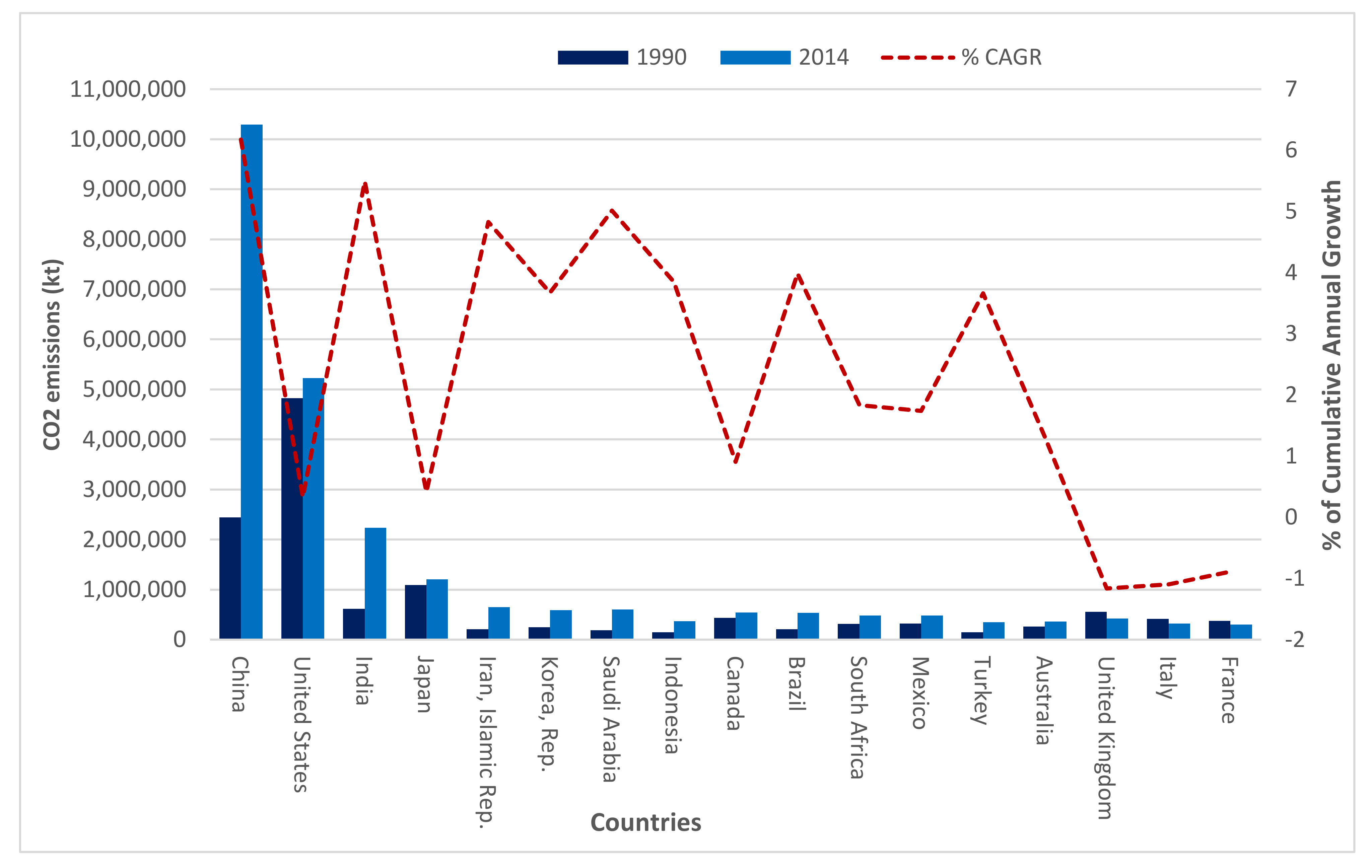
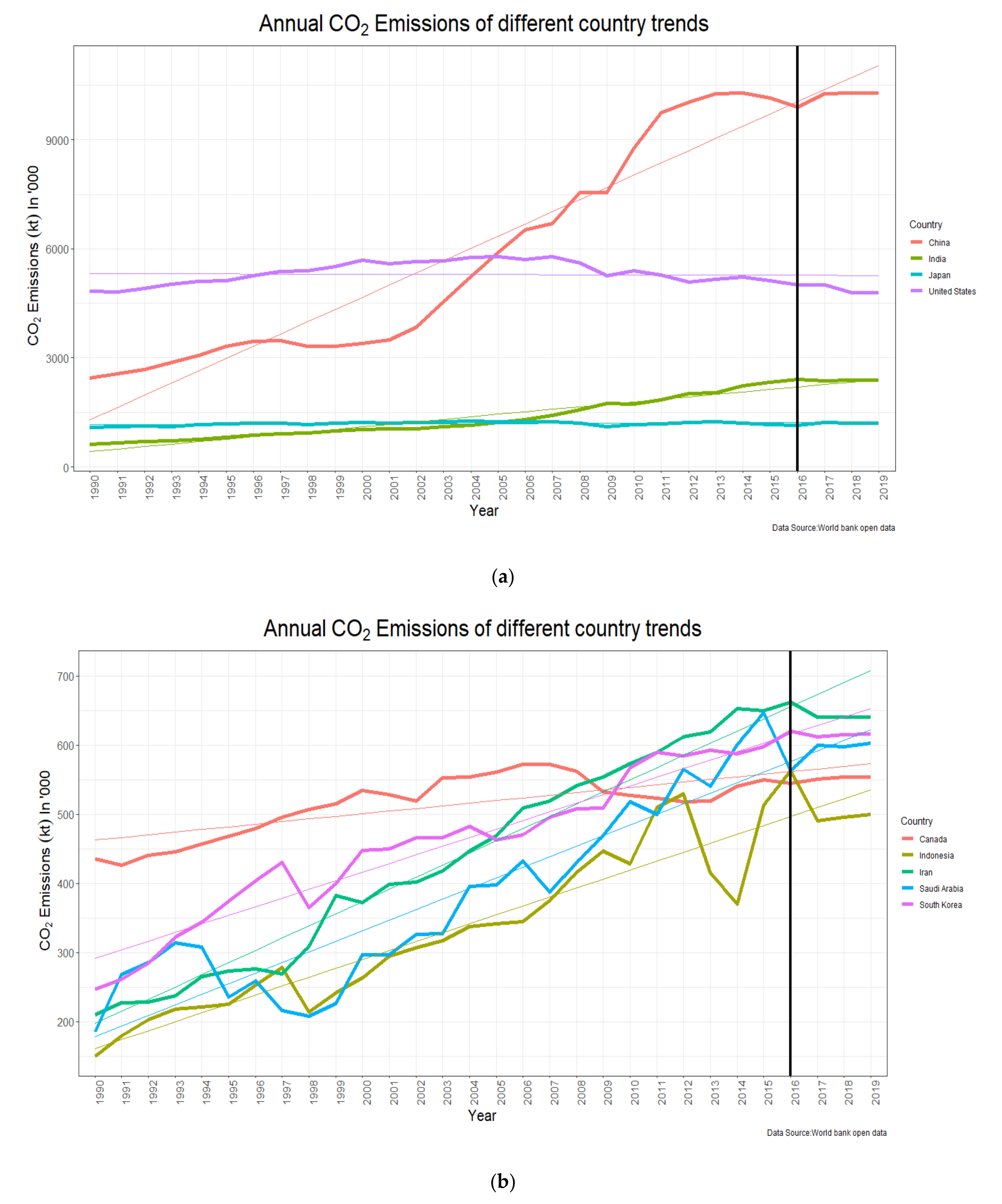
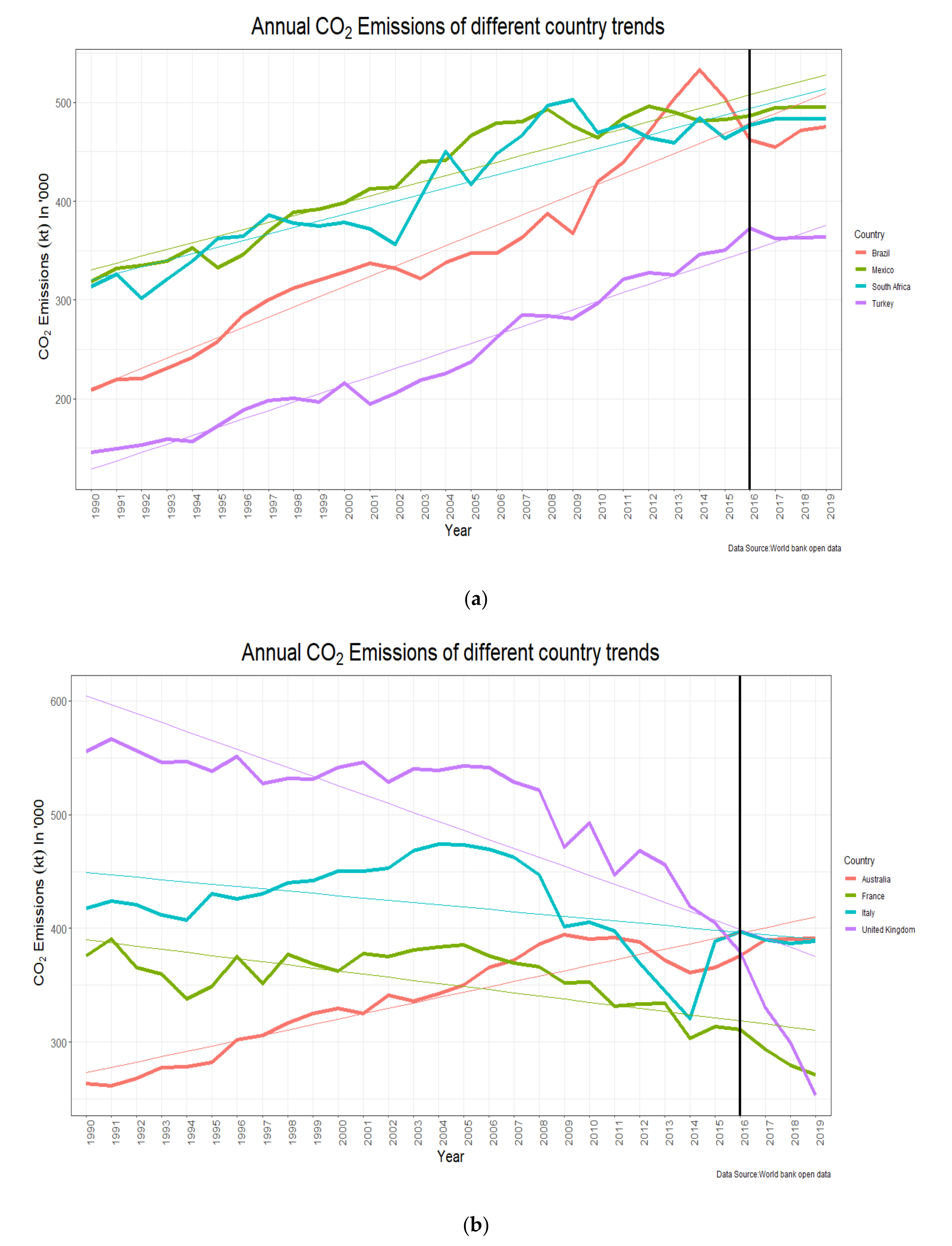
Figure 3 shows the CO₂ emissions of the 17 countries and their CAGR for the period 1990 and 2016. The countries that accounted for the highest growth in CO₂ emissions between 1990 and 2016 are China with 6.17%, India with 5.5%, Saudi Arabia with 5%, Iran with 4.8%, Brazil with 4%, and Turkey with 3.7%. The countries that have managed to rein in their emissions growth are UK with −1.16%, Italy with −1.1%, France with −0.88%, the USA with 0.33%, Japan with 0.41%, and Canada with 0.9%. The growth trends in Figure 2 and Figure 3 suggest that the highly developing countries tend to emit more CO₂ while the already developed countries have slowed down their emissions. This evidence for the period 1990–2016 is close to the assertions of the EKC.

However, future forecasts are needed to convince the developed countries to commit more financial support for the developing countries to motivate the latter to sacrifice some of their economic ambitions. The trade-off that the highly emitting developing countries, such as China, India, and Brazil have to accept to reduce their CO₂ emissions in order to comply with their commitments at the Paris climate summit agreement, is substantial. Unless they receive financial support from the industrialized countries as agreed upon by the Paris climate summit, these countries are unlikely to reduce their emission levels. We attempt to forecast the CO₂ emission levels of 17 countries that account for nearly 79% of the global emissions. By using the highly complex and non-linear artificial neural network (ANN) models that can accurately forecast the future emission values, we provide actionable insights to the policymakers to engage in more active dialogues to achieve the Paris agreement. Using the multilayer ANN model, we forecast the CO₂ emissions for Group 1 and 2 types of countries (Table 1) for 2017–2019.

3. Development of the Multilayer Artificial Neural Network (MLANN) Based CO₂ Forecasting Model

Statistical models are not able to estimate the relationships accurately when the data are uncorrelated, non-stationary, nonlinear and chaotic [32]. To overcome this problem various intelligent models are proposed by the researchers. The MLANN is a nonlinear, multi-layered, fully connected feedforward network that can model the nonlinearity of the data appropriately [33]. 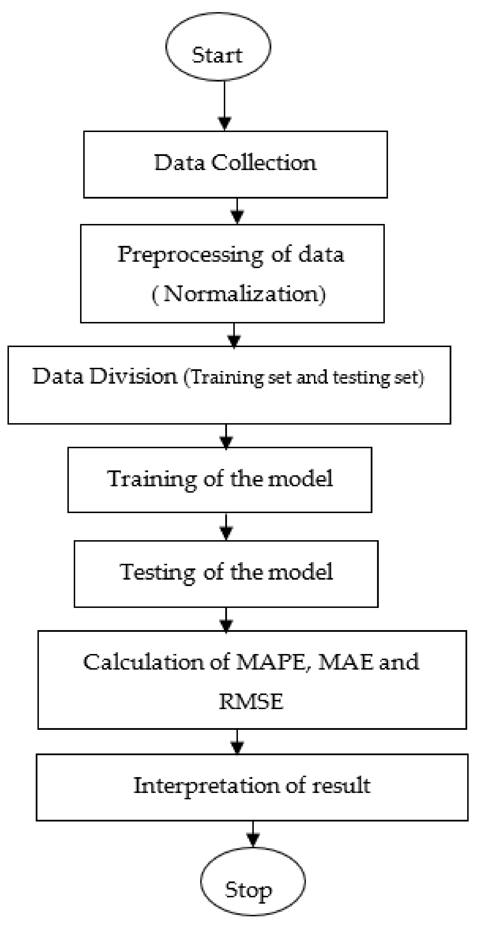The MLANN model is trained using past data and optimizes the weights that will be used to forecast the CO₂ emissions based on the inputs given. The flowchart shown in Figure 4 is used for the development of a MLANN based prediction model.

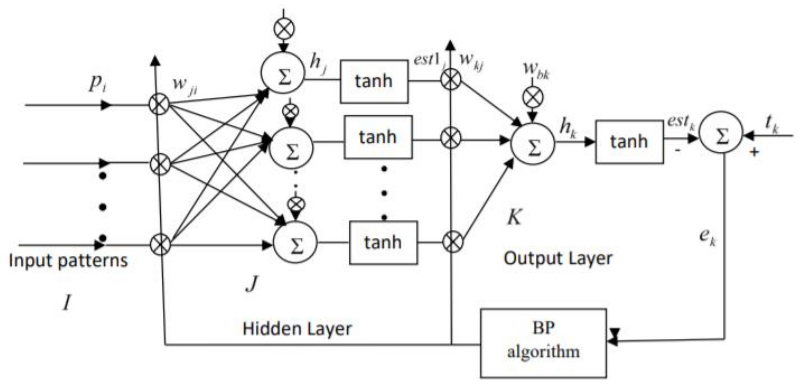
The complete structure of the MLANN based prediction model is given in Figure 5. Let $I,J\hspace{0.33em}and\hspace{0.33em}K$ represent the indices for the input, hidden and output layers respectively. Where $I$ = the number of inputs, $J$ = the number of neurons in the hidden layer, and $K$ = the number of neurons at the output layer. In this CO₂ prediction model the output is one value, so for this study the value of $K=1$. Let $P$ be the number of input patterns and let any $i\mathrm{th}$ input pattern is given as $p_i$. Each input pattern is supplied to the MLANN model sequentially, multiplied with the weights, sum together, and finally passed through the nonlinear activation function ($tanh$) to produce the output at the first hidden layer. This process is repeated for the next hidden layers and output layer. Let the estimated output of the network is $es{t}_k$. The error value is obtained by comparing the estimated value with the desired value or target value, $t_k$. The backpropagation learning rule [33] given in Equations (6)–(11) is used to update the weights and bias values of each layer. This process continues until the squared error is minimum. The detailed equations of feed-forward computation and rules to update the weights and bias are discussed below.

Refereeing to the above figure, the output of the $k\mathrm{th}$ output neuron $es{t}_k$ is given [33] as:

$$es{t}_k=\tan h(h_k)$$

(1)

Where

$$h_k={\displaystyle \sum }_{j=1}^{J}est{1}_j{w}_{kj}+w_{bk}\hspace{1em}$$

(2)

$est{1}_j=$ the output obtained at $j\mathrm{th}$ hidden neuron.

$w_{kj}=$ weights connecting $j\mathrm{th}$ hidden neuron and $k\mathrm{th}$ output neuron.

$w_{bk}=$ bias at $k\mathrm{th}$ output neuron.

In the same way, the output at neuron of $j\mathrm{th}$ hidden layer, $est{1}_j$ is computed [33] as—

$$est{1}_j=\tan h(h_j)$$

(3)

Where

$$h_j={\displaystyle \sum }_{i=1}^I{p}_i{w}_{ji}+w_{bj}\hspace{1em}$$

(4)

$$\begin{gathered} p_i=ith\hspace{0.33em}input\hspace{0.33em}pattern \\ {w}_{ji}=weights\hspace{0.33em}between\hspace{0.33em}ith\hspace{0.33em}input\hspace{0.33em}and\hspace{0.33em}jth\hspace{0.33em}hidden\hspace{0.33em}neuron \\ {w}_{bj}=bias\hspace{0.33em}at\hspace{0.33em}jth\hspace{0.33em}hidden\hspace{0.33em}neuron \end{gathered}$$

The error value is obtained by comparing the output of the prediction model, $es{t}_k$ with the corresponding target value, $t_k$. So,

$$e_k=t_k-es{t}_k$$

(5)

The weights connecting the neurons of hidden and output layers, $w_{kj}$ are updated [33] by:

$$w_{kj}=w_{kj}+\mu \times {\delta }_k\times est{1}_j\hspace{1em}$$

(6)

where

$${\delta }_k=e_k\times \frac{\left(1-es{t}^2{}_k\right)}{2}\hspace{1em}$$

(7)

$$\mu =learning\hspace{0.33em}parameter,\hspace{0.33em}(0<\mu <1)$$

The bias weight is updated as:

$$w_{bk}=w_{bk}+\mu \times {\delta }_k$$

(8)

Similarly, the weights connecting the input and the hidden layer neurons, $w_{ji}$ are updated [33] as:

$$w_{ji}=w_{ji}+\mu \times {\delta }_j\times p_i$$

(9)

where

$${\delta }_j={\delta }_k\times w_{kj}\times \frac{\left(1-est{1}_j{}^2\right)}{2}$$

(10)

The updating of bias weight of $jth$ neuron in the hidden layer is done [33] as:

$$w_{bj}=w_{bj}+\mu \times {\delta }_j\hspace{1em}$$

(11)

The Equations (1)–(11) are the key equations used in the development of the MLANN based CO₂ forecasting model.

4. Simulation study

The CO₂ emissions prediction is formulated as an optimization problem. The model is having three inputs and one output. The inputs are fed to the model and the obtained output is compared with the available target value until the squared error is minimum. Matlab 2016 package is used for the simulation of the problem.

(a)

Data collection and preprocessing:

The data for 9 countries under Group 1 and 8 countries under Group 2 are collected from 1960 to 2016 till which the comprehensive data are available in the World Bank database. CO₂ emissions are used as the output parameter for which the out-of-sample forecasting has been done. The variables, such as GDP (in constant 2010 US$), trade ratio, and urban population are used as the inputs in the MLANN model. The data has been preprocessed as the first step in the modeling wherein the data for all the variables have been normalized. During normalization, each value of the four variables is divided by the corresponding maximum value so that all values can lie between 0 and 1. Normalized data generally makes the learning process and the convergence speed faster. If all features do not have similar ranges of values, then the gradients can move to and fro and take a long time before they can attain the global minimum. To circumvent this problem in the learning process, normalization of the data is necessary. Normalization of the data is followed by preparation of training set and testing set. Randomly selected 80% of data are used for training of the model and the rest 20% of data is used for testing of the developed model. Simulation is carried out by varying the ratio of data division (70:30, 80:20, and 90:10) and an 80:20 ratio is selected finally as it gives the best result. Further, the three missing values of CO₂ emission for the year 2017–2019 are calculated using the optimized weights of MLANN based model.

(b)

Training of the model:

Out of the total of 57 patterns (1960 to 2016), the training set consists of 46 patterns that are randomly chosen, and the remaining 11 patterns are used for testing of the calibrated model. An input pattern of data consists of the values of trade ratio, urban population, and GDP. The corresponding CO₂ emission value is the target value for the training of the model. A 9:3:1 structure is used for the simulation. It consists of two hidden layers with nine and three neurons respectively. The connecting weights between the layers and the bias weights are randomly initialized to lie between −0.5 to 0.5. The 9:3:1 structure is fixed after doing experiments by varying different structures of MLANN as it gives minimum error value. In each iteration, one input pattern is given to the model, and feedforward processing is done to get the estimated output from the model. Feedforward processing involves summing the weighted inputs, adding the bias weights, and then passing it through the activation function or nonlinear function (tanh). The estimated output is compared with the corresponding target value to obtain the error. The backpropagation (BP) training algorithm is used to update the connecting weights and bias weights. The value of the learning parameter is taken as 0.1. The same process is repeated until all training patterns are exhausted. This completes one experiment. The experiment is repeated until the mean squared error (MSE) is minimized. The MSE value for each experiment is stored and plotted to observe the convergence characteristics. The final value of connecting weights and bias weights are frozen for testing of the developed model.

(c)

Testing of the model:

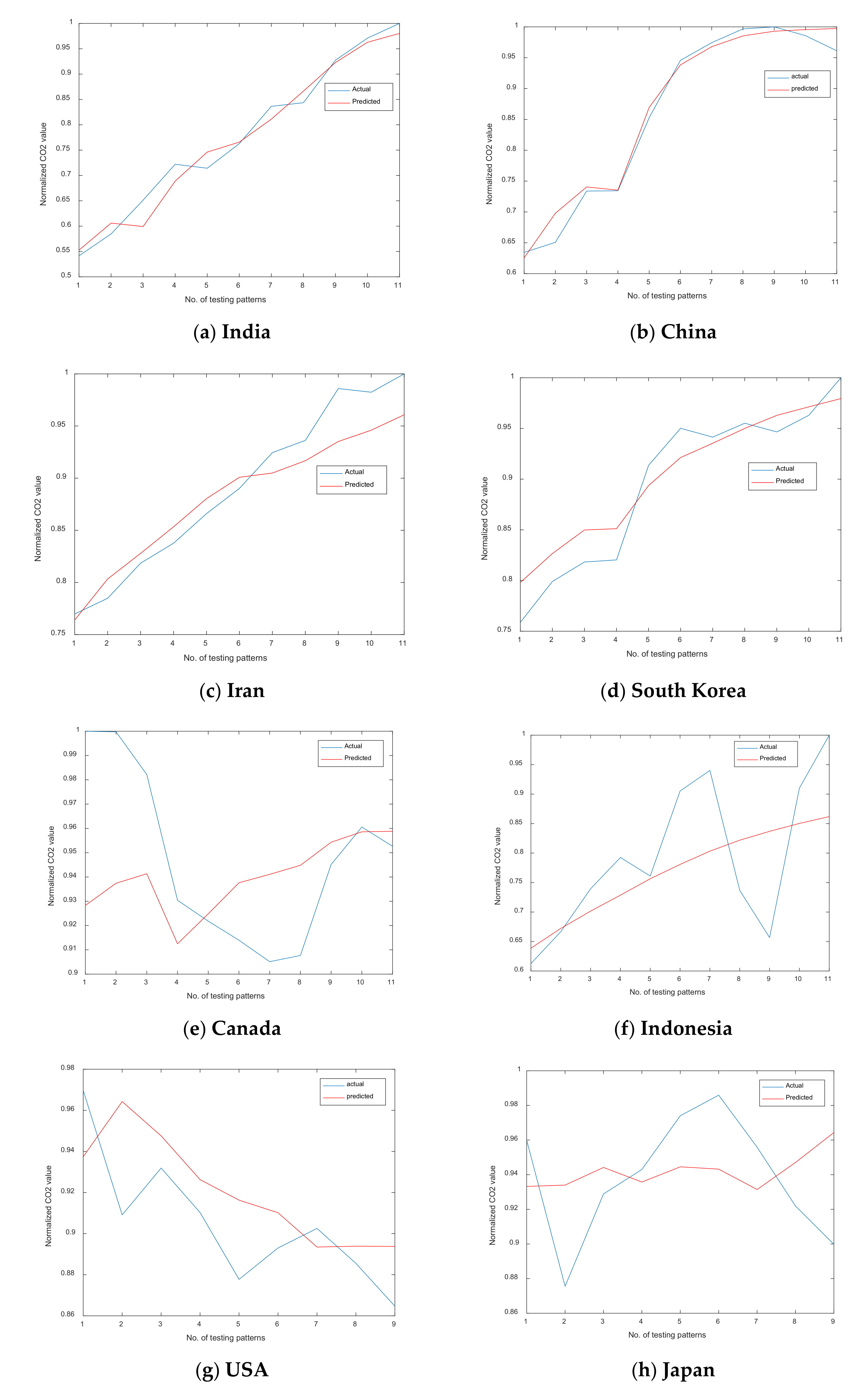
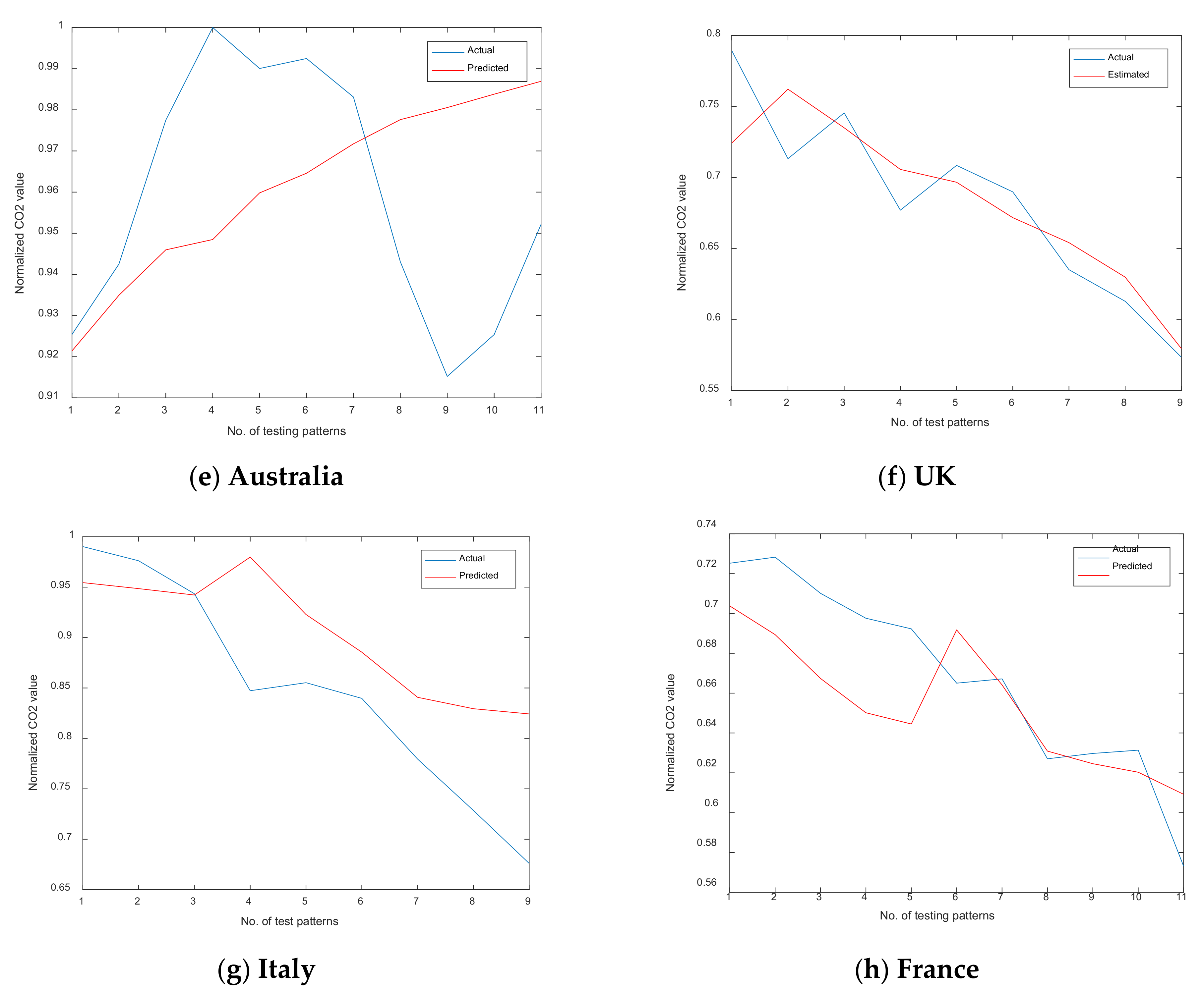
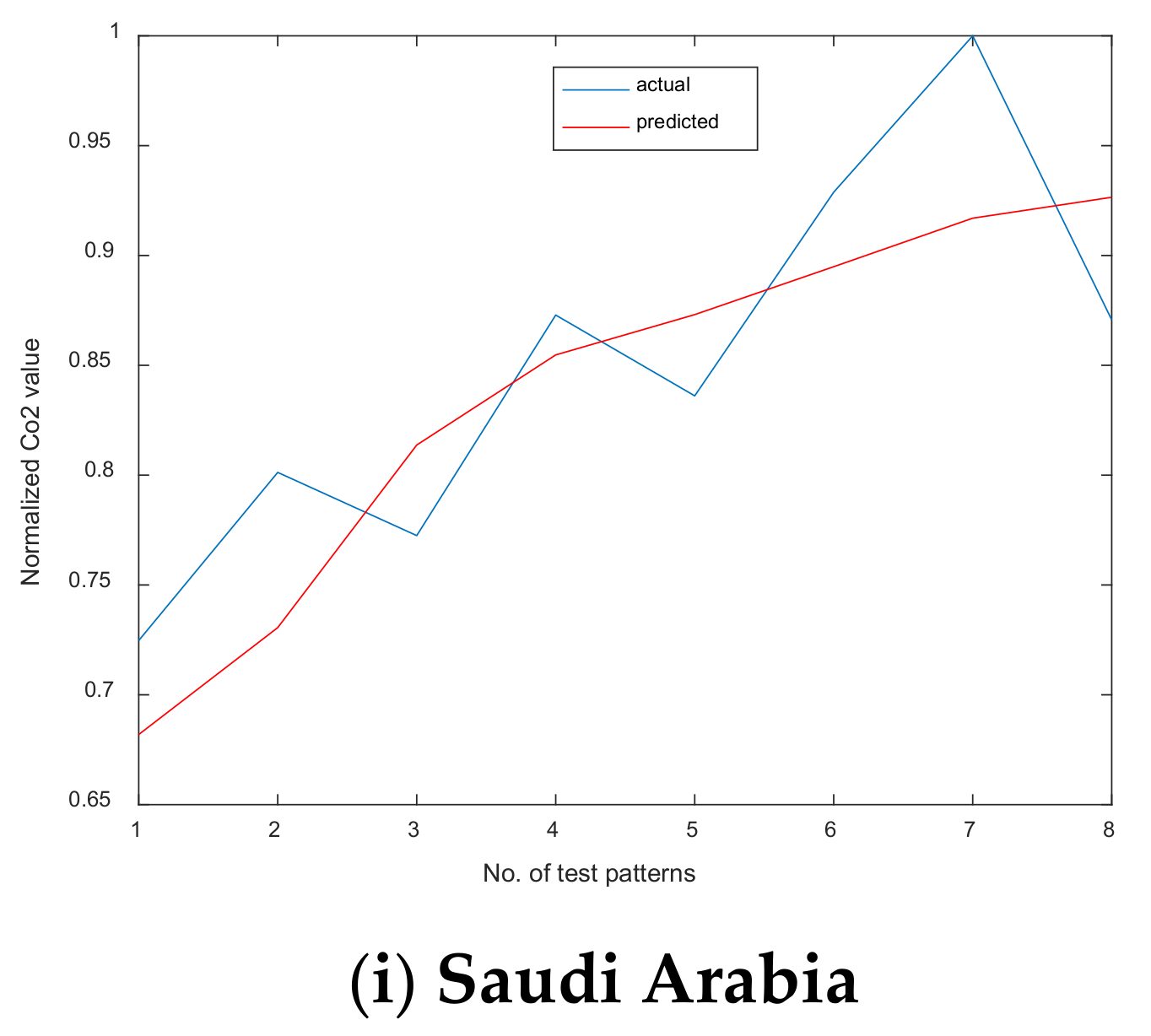
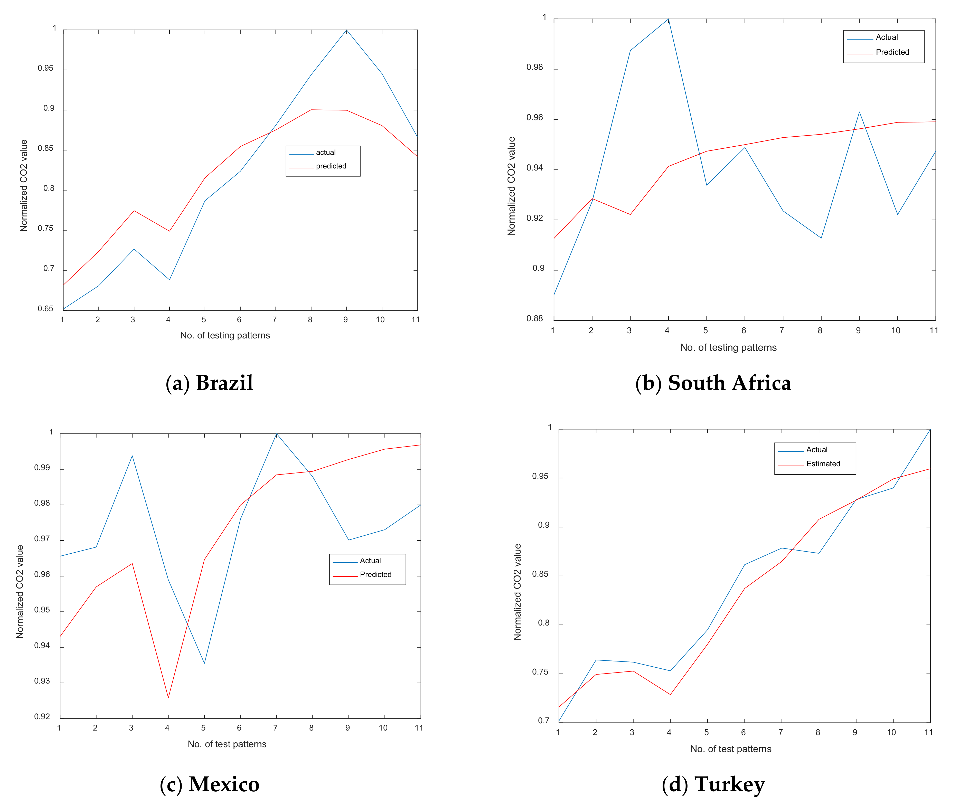
Once the training process is complete, the developed MLANN based model is ready to be used for evaluation. The 20% of the testing patterns are applied to the model sequentially and the estimated output is noted. The estimated output is compared with the corresponding desired value and the mean absolute percentage error (MAPE), mean absolute error (MAE) and root mean square error (RMSE) are tabulated in

Table 2. MAPE, MAE and RMSE values obtained during testing for Group-1 countries.

Sl. No.	Name of Country	No. of Total Data Samples Available	MAPE Values(%)	MAE	RMSE
1	India	57 (1960–2016)	2.9287	0.0198	0.0235
2	China	57(1960–2016)	1.7896	0.0113	0.0150
3	Iran	57(1960–2016)	2.3610	0.0262	0.0277
4	South Korea	57 (1960–2016)	2.4803	0.0244	0.0324
5	Canada	57 (1960–2016)	2.9358	0.0244	0.0277
6	Indonesia	57 (1960–2016)	9.6898	0.0767	0.1077
7	USA	47 (1970–2016)	2.7168	0.0265	0.0308
8	Japan	47(1970–2016)	3.5206	0.0214	0.0264
9	Saudi Arabia	49 (1968–2016)	5.9153	0.0462	0.0535

and

Table 3. MAPE, MAE and RMSE values obtained during testing for Group-2 countries.

Sl. No.	Name of Country	No. of Total Samples	MAPE (%)	MAE	RMSE
1	Brazil	57 (1960–2016)	5.3345	0.0330	0.0412
2	South Africa	57 (1960–2016)	2.7524	0.0279	0.0379
3	Mexico	57 (1960–2016)	1.9266	0.0200	0.0224
4	Turkey	57 (1960–2016)	2.1538	0.0162	0.0209
5	Australia	57 (1960–2016)	3.4001	0.0367	0.0417
6	UK	47(1970–2016)	3.5419	0.0410	0.0502
7	Italy	45(1970–2014)	8.8015	0.0653	0.0769
8	France	55(1960–2014)	3.8158	0.0241	0.0333

which indicate the performance of the model. The MAPE, MAE and RMSE are calculated using Equations (12)–(14). Also, the comparison of the actual and estimated CO₂ values during testing are plotted and exhibited in Figure 6a–i for Group-1 countries. For Group-2 countries, it is given in Figure 7a–h.

$$MAPE=\frac{1}{n}{\displaystyle \sum }_{i=1}^n\frac{\left|(t\left(n\right)-est\left(n\right)\right|}{t\left(n\right)}\times 100$$

(12)

$$MAE=\frac{1}{n}{\displaystyle \sum }_{i=1}^n\left|(t\left(n\right)-est\left(n\right)\right|$$

(13)

$$RMSE=sqrt\left(\right.\frac{1}{n}{\displaystyle \sum }_{i=1}^n{(t\left(n\right)-est\left(n\right))}^2\left.\right)$$

(14)

$$MAPE=\frac{1}{n}{{\displaystyle \sum }}_{i=1}^n{\frac{\left|(Ou{t}_{obs}-Ou{t}_{est})\right|}{Ou{t}_{obs}}}_{\times 100} \mathrm{where} t\left(n\right)=\mathrm{target} \mathrm{value}$$

$$est\left(n\right)=\mathrm{estimated} \mathrm{value}$$

$$n=\mathrm{Number} \mathrm{of} \mathrm{testing} \mathrm{patterns}$$

5. Results and Discussion

From Table 2 it is observed that the MAPE values for Group-1 countries lie between 1.78 to 3.52% except for Indonesia and Saudi Arabia. The MAPE value is 5.91 for Saudi Arabia and 9.68 for Indonesia. The MAPE is an indicator of how close the predicted values are to the actual values. The RMSE values lie between 0.01 to 0.05 for Group I countries except for Indonesia. The MAE values lie between 0.01 to 0.07 for Group I countries. The MAPE values for the Group-2 countries are given in Table 3 which shows that the values lie between 1.92 and 3.8 except for Brazil and Italy. The value is 5.33 for Brazil and 8.08 for Italy. The RMSE values lie between 0.02 to 0.07 and the MAE values lie between 0.01 to 0.06 for Group II countries. As the MAPE values are less than 4% for most of the countries considered in this study, the MLANN model is able to predict the values reasonably accurately with less percentage of error except for a few cases. The comparison of actual and estimated CO₂ values obtained during testing is shown in Figure 6 and Figure 7 for Group-1 and Group-2 countries respectively. In most cases, the actual and estimated values are close to each other.

However, the gap between the actual and predicted values of CO₂ emissions found during the testing phase of the model for Indonesia, Saudi Arabia, Brazil, and Italy is due to the wide fluctuations observed in their emissions data during the period of the study. Although the MLANN model developed in this study is robust to the nonlinearities in the data, wide fluctuations may still increase the percentage of error as is the case for these four countries.

The simulation study is carried out by varying the ANN structure. Different combinations of hidden layer and neurons are used to simulate the model and the results in terms of the training and testing times, as well as the performance achieved, are obtained and displayed in Table S1 in Supplementary Materials. For each country data, initially, combinations of one hidden layer where five, six, seven and eight neurons are used, and thereafter two hidden layers with the same variations of neurons are used for simulation. From Table S1 in Supplementary Materials, it is exhibited that comparing the training time, testing time, MSE in training, and MAPE in testing, the proposed structure of the MLANN model is better in comparison to other combinations of hidden layer and neurons. Further, the simulation is also carried out with different data division ratios and it is observed from Tables S2 and S3 in Supplementary Materials, that the 80–20% ratio is suitable for the proposed study as it gives the minimum MAPE value in all cases.

As suggested in Wu et al. [34], other machine learning methods, such as the support vector machine (SVM) model is simulated and the resultant MAPE values are provided in Table S4 in Supplementary Materials. It is observed that the MAPE values of all countries of Group-I and Group-II are higher in comparison to the proposed MLANN model. We have not added the methods of SVM and a detailed comparison between MLANN and SVM in the main text since it will require substantial expansion of the manuscript.

Forecasting of CO₂ Emissions

In this section, we present the forecasted values of CO₂ emissions for the Group-1 and Group-2 countries for the years 2017, 2018, and 2019 given in

Table 4. Forecasted CO₂ emission values for the year 2017–2019 for Group-1 countries.

Sl. No.	Name of Country	Year	CO2 Emission Values (in kt)
1	India	2017 2018 2019	2.3775 × 106 2.3858 × 106 2.3913 × 106
2	China	2017 2018 2019	1.0275 × 107 1.0279 × 107 1.0281 × 107
3	Iran	2017	6.4003 × 105
4	South Korea	2017 2018 2019	6.1217 × 105 6.1490 × 105 6.1616 × 105
5	Canada	2017 2018 2019	5.5083 × 105 5.5332 × 105 5.5369 × 105
6	Indonesia	2017 2018 2019	4.9101 × 105 4.9581 × 105 4.9984 × 105
7	USA	2017 2018	5.0148 × 106 4.8022 × 106
8	Japan	2017 2018	1.2187 × 106 1.2115 × 106
9	Saudi Arabia	2017 2018 2019	5.9955 × 105 5.9752 × 105 6.0329 × 105

and

Table 5. Predicted CO₂ emission values for the year 2017–2019 for Group-2 countries.

Sl. No.	Name of Country	Year	CO2 Values (in kt)
1	Brazil	2017 2018 2019	4.5462 × 105 4.7165 × 105 4.7525 × 105
2	South Africa	2017 2018 2019	4.8368 × 105 4.8349 × 105 4.8327 × 105
3	Mexico	2017 2018 2019	4.9500 × 105 4.9521 × 105 4.9517 × 105
4	Turkey	2017 2018 2019	3.6217 × 105 3.6326 × 105 3.6368 × 105
5	Australia	2017 2018 2019	3.9027 × 105 3.9094 × 105 3.9122 × 105
6	UK	2017 2018 2019	3.3021 × 105 2.9951 × 105 2.5307 × 105
7	Italy	2015 2016 2017 2018 2019	3.8895 × 105 3.9707 × 105 3.9028 × 105 3.8698 × 105 3.8842 × 105
8	France	2015 2016 2017 2018 2019	3.1387 × 105 3.1091 × 105 2.9378 × 105 2.7934 × 105 2.7095 × 105

respectively. These are out-of-sample forecasts of CO₂ emissions based on the optimized weights from the calibrated MLANN model and the values for inputs, such as GDP (in 2010 constant US$), urban population, and trade ratio for 2017, 2018, and 2019. The data of CO₂ emissions for these years are not available, however, the data for inputs for these three years are available for most of the countries considered in this study except for Iran, the USA, and Japan. For Iran, input data is available only for 2017, and for the USA and Japan, it is available for 2017 and 2018. Accordingly, the forecasts are done for these countries for the years the input data are available. The EKC hypothesis stands on the empirical evidence that the elasticity of income effect is larger than the combined elasticities of scale and composition effects [35,36]. The literature review in this study has discussed many recent articles that have either established the EKC relationship in the long run or failed to find evidence for it. A few other studies have used a similar framework as EKC to forecast the out-of-sample values of CO₂ emissions [37]. Aufhammer and Carson forecasted the CO₂ emissions for the Chinese provinces for the single year of 2010 by using the estimated coefficient values of different predictors of their ‘best’ model and the projected values of the predictors, such as GDP per capita and population figures whose values were unknown when they published this study. Two other noteworthy studies by [38] and [39] have used a similar approach and forecasted the time path of CO₂ emissions for the year 2100 and 2050 respectively. We improve upon these studies in two ways. First, we develop a sophisticated neural network nonlinear model to calibrate the EKC relationship and obtain the optimized input weights that are used to predict the CO₂ emissions based on the predictors, such as GDP, urban population, and trade ratios. These optimized weights provide a more realistic time-series relationship between the emissions and the predictors. Secondly, we forecast the CO₂ emissions for high emitting and low emitting countries based on the known values of the predictors, not their projected values.

Figure 8a,b depict the CO₂ emission values for the Group-1 countries from 2010 to 2019. The emissions from 2010 to 2016 are the actual data obtained from the World Bank database, whereas the values from 2017 to 2019 are the forecasted values. Figure 8a shows that the forecasted emissions for both China and India have increased. China surpassed the USA in 2005 and since then the rate of emission growth is substantially higher for China. During the same period of 2005–2019, the USA’s emissions levels have dipped and during the short period of 2017–2019, it shows a declining trend. This is a noteworthy observation in the context of international climate negotiations. Although the USA is not a signatory to Paris climate agreements, it has its internal pollution regulation mandates that have yielded a reduction in CO₂ emissions. On the other hand, China has taken great strides in transforming its economic structure following a circular economy model [40]. Despite these reforms, the emission levels are expected to rise in the short-run horizon. China’s past high emission levels and the high growth rate in emission will render it a high emitting country in the near future despite its significant improvement in restructuring the economic models. India is the third highest CO₂ emitter in the world and the rate of emission growth shows a rising trend for the country. The forecasted values for 2017–2019 signify the uphill challenge India is facing to comply with its commitments towards Paris agreements as the emission levels are expected to rise during this period. Japan’s emission levels are predicted to reduce further following its declining trend that started around 2007.

Figure 8b shows that the trajectory of CO₂ emissions in Indonesia is quite volatile which is the reason for a higher percentage error in our forecasts for Indonesia. The forecasted values for the period 2017–2019 show arising rend for the country. The other countries in the Group-1 category that shows a rising expected level of CO₂ emissions are Iran, South Korea, and Saudi Arabia. Whereas Canada’s emission levels have been stabilized and it embarked on a declining phase of CO₂ emissions since 2008. Figure 9a shows the CO₂ emission trajectory and the forecasted levels for the Group-2 countries. Although the global share of CO₂ emission in countries, such as Brazil, South Africa, Mexico, and Turkey are either 1% or less than 1%, their expected emission level will rise in the near future. Brazil, in particular, shows a high emission growth path which weakens the country’s position in the future global climate summits, such as COP26. The reported burning of large tracts of Amazonian forest in Brazil has been heavily criticized by the rest of the globe. The country needs to be more proactive and engaged in complying with its Paris agreement commitments. The expected trajectory of the CO₂ emission growth path for the industrialized countries, such as France, the UK, Australia, and Italy are shown in Figure 9b. The emission levels in France and UK are continuously declining and are expected to decline further. Italy and Australia have reached their peak levels of CO₂ emission in 2006 and 2011 respectively. Since then, their emission levels have stabilized at lower levels and are expected to decline further.

6. Conclusions

The IPCC report [41] warns that the current level of national pledges on mitigation of greenhouse gas emissions and adaptation to climate change are not enough to constrain global warming to the level agreed upon by the countries in the Paris Agreement. The report urges the signatory countries to upscale and accelerates the implementation of multilevel and cross-sectoral climate mitigation actions. To be able to do so, accurate prediction of future CO₂ emission path in business-as-usual conditions holds importance. Such predictions would lead the countries to accelerate their mitigation and adaptation measures. This study forecasts the CO₂ emissions for the high and low emitting countries by their global shares of emission, for the years 2017, 2018, and 2019. Among the high emitting countries, China and India have been treading a high emission growth path, whereas the US and Japan are on the declining trend. Following the EKC hypothesis literature, we model the CO₂ emissions as the output of the model and GDP in constant 2010 US$, urban population, and trade ratios as the predictors. Several past studies have used the same variables to predict the EKC relationship, however, their methods had been static and mostly linear. Considering that the relationship between CO₂ emissions and its predictors may be nonlinear in the long run, we develop a multilayer artificial neural network model to estimate this relationship.

Based on the World Bank database of 17 countries, of which nine are placed in high emitting (Group-1) and the remaining eight in the low emitting (Group-2) countries spanning from 1960 to 2016, a MLANN model is developed. After the model simulation, it is observed that the prediction accuracy of the in-the-sample data has been 96% leaving 4% to the prediction error. With this high level of prediction accuracy, the model is well calibrated to forecast the out-of-the-sample emission growth path. The data for the input predictors have been available for the years 2017, 2018, and 2019 but not for the CO₂ emissions of the selected countries. Hence, we forecast the CO₂ emissions of these years based on the optimal weights and the input data. From the results, it is observed that China despite its aggressive transformation of economic activities to a circular economy model, is still on the path of increasing emissions in near future. Similarly, India will continue to emit higher levels of CO₂ in the short run that has been studied. Other high emitting countries, such as Iran, Indonesia, Saudi Arabia, and South Korea are expected to continue with their high CO₂ emission growth path if they remain on the BAU economic production-consumption trajectory. These countries need to restructure their economic activities in more sustainable ways to reduce greenhouse gas (GHG) emissions. However, the US and Japan are expected to further reduce their carbon footprint by emitting less CO₂ into the atmosphere. France, UK, Italy, Australia, and Canada are poised to stabilize their emission levels at a low emission growth path and are on course to comply with the Paris agreement. Finally, although low emitting countries, Brazil, South Africa, Turkey, and have been on the rising path of GHG emissions. These countries prioritize their economic growth over the reduction of CO₂ emissions. Hence, they are not expected to comply with the Paris agreement’s emission reduction goals.

Based on these results, it is incumbent upon the national policymakers and multilateral policy supporting bodies, such as the UN, OECD, World Bank, and IMF to commit more financial resources for the reduction of CO₂ emissions. Most of the countries that we studied that are on a high emission growth path are currently industrializing. Their goal is to achieve higher economic growth, create more employment, and increase income per capita. Hence, these countries are less likely to change their economic structure suitable for a low carbon economy. The already industrialized countries who have achieved a reduction in their national CO₂ emission goals must come forward to support the countries who are not close to achieving the pledges they made at the Paris climate conference. The next multilateral climate summit which is scheduled to take place in the UK in October-November 2021, known as COP26 will have to focus on issues of greater climate cooperation and finance.

The MLANN model used in the study though has forecasted the CO₂ emission quite accurately in most cases, there are a few cases where the prediction error was high. This is a limitation of the study. Future studies can use other ANN-based models like radial basis function neural network (RBFNN), recurrent neural network (RNN), extreme learning machine (ELM), etc., to reduce the percentage of error. Further, the scope of this study can be expanded by using the mean impact value (MIV) based method to select features and by using the optimal lag order of input data as suggested by Lee and Ou [42] and Wu et al. [43].