Research on the State of Charge of Lithium-Ion Battery Based on the Fractional Order Model

Abstract

Accurate estimation of the state of charge (SOC) of lithium batteries is paramount to ensuring consistent battery pack operation. To improve SOC estimation accuracy and suppress colored noise in the system, a fractional order model based on an unscented Kalman filter and an H-infinity filter (FOUHIF) estimation algorithm was proposed. Firstly, the discrete state equation of a lithium battery was derived, as per the theory of fractional calculus. Then, the HPPC experiment and the PSO algorithm were used to identify the internal parameters of the second order RC and fractional order models, respectively. As discovered during working tests, the parameters identified via the fractional order model proved to be more accurate. Furthermore, the feasibility of using the FOUHIF algorithm was evaluated under the conditions of NEDC and UDDS, with obvious colored noise. Compared with the fractional order unscented Kalman filter (FOUKF) and integer order unscented Kalman filter (UKF) algorithms, the FOUHIF algorithm showed significant improvement in both the accuracy and robustness of the estimation, with maximum errors of 1.86% and 1.61% under the two working conditions, and a terminal voltage prediction error of no more than 5.29 mV.

1. Introduction

Currently, the traditional automobile industry is one of the main contributors to the global greenhouse effect and oil crisis, and consequently the development of new electric vehicles is evolving. To this end, many automobile companies have transformed themselves and issued a timetable for ending the sale of traditional fuel vehicles. The new vehicle models are mainly battery electric vehicles (BEV), hybrid electric vehicles (HEV) and plug-in hybrid electric vehicles (PHEV). The main types of power batteries currently available for electric vehicles include lead-acid, nickel-chromium, nickel-hydrogen, and lithium-ion batteries. Between them, lithium-ion batteries have the highest specific energy and volumetric specific energy, in addition to a long service life [1,2]. SOC is an important lithium battery parameter and an accurate SOC estimation can help improve the service life and battery safety.

There are four methods employed in SOC estimation. Firstly, there is the Coulomb counting method. Although the calculation is simple, there are also obvious drawbacks. For example, it is difficult to determine the initial calculated value, so it is generally used in combination with an open-circuit integral method. However, before using this method, the lithium battery needs to be left to set for a long time and the current sensor may also show errors. When mixed with noise from the external environment, the current error accumulation will continue to increase [3]. The second method is through empirical value-based estimation, represented by neural networks, fuzzy algorithms, and support vector equipment. The neural network requires a large amount of training data in the early stages to explore the relationship between various parameters in the nonlinear system with high estimative accuracy. However, this method also has distinct shortcomings, namely, the primary task of inputting a large amount of training data into the system means that the estimation cannot be made in real time, and so this method has poor adaptability as realistically it can only be used in a training environment. Furthermore, fuzzy algorithms also need to process a large amount of data in the early stages, which is difficult to implement in an embedded system [4]. Marvin Messing et al. took the internal parameters of a battery model as the input values of a neural network. The experimental results showed that the SOC estimation was relatively ideal [5]. Yin et al. adopted a PSO algorithm to optimize the weight and threshold of the neural network, and subsequently used a SA algorithm to optimize the PSO algorithm. The experimental results revealed that the PSO algorithm was optimized for both accuracy and arithmetic speed [6]. Darsana Saji et al. solved the problem of error accumulation by using a combination of the coulomb counting method and the fuzzy algorithm, achieving high robustness and improved estimation accuracy [7]. The third method is an estimation process based on the battery characterization parameters. It is mainly used in laboratory environments to identify the relationship between the parameters (including the open-circuit voltage and remaining capacity) and the SOC of the lithium battery. This method is convenient and accurate, but not suitable for practical application. Liu et al. estimated the SOC by using battery characterization parameters such as the rebound voltage and temperature in combination with a neural network. The results demonstrated that the estimated SOC values in this method were highly accurate and consistent under various working conditions [8].

The fourth approach is an estimation method that combines filtering theory with an equivalent circuit model, and is currently the most popular and reliable method [9,10]. The common filtering algorithms include the Kalman filter algorithm [11], H infinite filter algorithm [12] and so on. The main advantage with these algorithms is that it is not necessary to stage the battery for long periods or to train the data before use. Moreover, real-time correction can be made in the case of errors in the theoretical and measured values to conclusively estimate an accurate SOC. Amongst the filtering algorithms, the unscented Kalman filter (UKF) algorithm develops quickly, and its UT transformation link can usually be improved by obtaining more accurate values of the estimated parameter. H. Aung et al. adopted an improved square root UKF algorithm, where the arithmetic speed was improved by reducing the amount of sigma points [13]. Another research focus of the UKF algorithm is its noise covariance matrix, with relevant theories showing that UKF noise should be assumed in advance. Accordingly, Peng [14] and Sun [15] used an adaptive UKF algorithm to estimate the SOC of lithium batteries, and adjusted the noise covariance matrix in real time, which contributed to the fast convergence of the algorithm. In the process of SOC estimation, the largest problem often comes from colored noise interference. The main filtering algorithms suitable for colored noise estimation include the H infinity algorithm [16]. Liu et al. proposed an adaptive H-infinity algorithm, which could not only help to filter out colored noise but also solved the problem of the inaccurate initial values of the noise covariance matrix. Moreover, the estimation accuracy was improved [17]. Liu et al. used a method combining the UKF algorithm with an H-infinity algorithm, where the UKF algorithm was used to linearize the nonlinear system. The experimental results proved that this combined method could compensate for sensor errors [18].

Presently, equivalent circuit models are normally divided into integer order models and fractional order models. The contents of the previous paragraph all relate to integer order models. Compared with integer order models, fractional order equivalent circuit lithium battery models can more comprehensively depict the internal chemical reaction mechanism of the battery, resulting in improved SOC estimation accuracy [19,20]. Mu et al. established a fractional order model which is simplified to be similar to the Thevenin model, and on this basis a fractional order UKF technology was derived [21]. Additionally, Chen et al. established a fractional second-order RC equivalent circuit model, and based on this model, a fractional order UKF technology was developed [22]. In terms of updating the covariance matrix, the technology developed by reference [22] is different from that derived by reference [21], but is more effective.

In view of the obvious advantages of the fractional order model over the integer order model, a fractional order lithium battery model based on the FOUHIF estimation algorithm is proposed in this paper. The specific layout of this paper is as follows: Section 2 gives a detailed introduction to the fractional order lithium battery model; Section 3 describes the identification of the internal parameters of integer order battery and fractional order battery models, and compares their respective effects; Section 4 initially introduces and analyzes the UKF and H infinity (HIF) algorithms, then proposes a fractional order model-based unscented and H-infinity (FOUHIF) estimation algorithm; Section 5 describes the experiment carried out under complex working conditions and compares the performances of the FOUHIF algorithm, the fractional order unscented Kalman filter (FOUKF) algorithm, and the integer-order unscented Kalman filter (UKF) algorithm.

2. Lithium Battery Modeling

In reference [23], a new linear capacitance model was proposed based on Curie’s empirical law. Curie’s empirical law states that when a DC voltage U is applied to two ends of a capacitor at the initial moment, the current generated by the capacitor complies with the relationship equation $i(t)=U/(h_1{t}^n)$, where, h₁ and n are constants, and 0 < n < 1. This law is an empirical relationship. The newly proposed capacitance model can be summarized as follows: $i(t)=C\frac{d^{n}u(t)}{d{t}^n},0<n<1,t>0$, and it was revealed that there is no constant capacitance in practical engineering. These theories also imply that the essence of capacitance is fractional order.

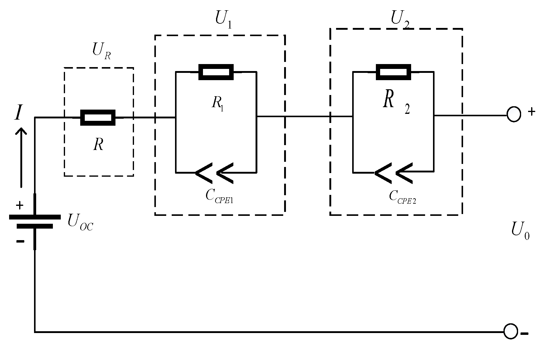
In engineering, the complex chemical reaction mechanism in lithium batteries is often depicted by establishing an equivalent battery circuit model for simplicity’s sake to clarify physical meaning and for online use. The main equivalent circuit models are the Rint, Thevenin, PNGV, and multi-order RC models. However, they all have a common drawback. That is, integer order models cannot depict the charge transfer reaction between the electrolyte and the solid-phase interface layer or the electrochemical process of the electric-double-layer effect. This implies that test results obtained over multiple testing cycles under working conditions severely deviate from the true value. Consequently, in this research, the second order RC model was improved into a fractional order model that can depict the reaction mechanism more realistically. The improved model is shown in Figure 1, where R₀ is the ohmic internal resistance of the battery, which reflects its ohmic polarization characteristics; the fractional order links formed by the constant phase elements CPE1 and R₁ describe the charge transfer process and the electric-double-layer effect in the battery electrochemical processes; the fractional order links formed by the constant phase elements CPE2 and R₂ describe the transfer reaction behavior between the electrolyte and the solid phase interface during the battery electrochemical processes.

There are three common definitions of fractional calculus: the Riemann–Liouville (RL) definition, the Caputo (CP) definition, and the Grünwald–Letnikov (GL) definition [24]. Since the GL definition is concise and clear, it is more appropriate for engineering, and it is also easily combined with the Kalman filter algorithm. Therefore, in this paper, the GL definition is used to establish the fractional-order lithium battery model. The GL definition is given as:

$${}_{\alpha }{D}_t^{r}f(t)=\underset{ h\to 0}{\lim }{h}^{-r}{\displaystyle \sum _{i=0}^{\left[\frac{t-a}{h}\right]}{(-1)}^i\left(\begin{array}{c}r\\ i\end{array}\right)f(t-ih)}$$

(1)

$${}_{\alpha }{D}_t^{r}f(t)=\{\begin{array}{c}{d}^{r}f(t)/d{t}^r\begin{array}{cc}& r>0\end{array}\\ 1\begin{array}{cc}& r=0\end{array}\\ {\displaystyle {\int }_{\alpha }^{t}f(t){(dt)}^{-r}}\end{array}$$

(2)

In the equation, ${}_{\alpha }{D}_t^r$ represents a continuous integral differential operator, where α, t are the upper and lower limits of the integral, and r is the fractional order of each link. The impedance of the two constant phase elements (CPEs) in the above figure is expressed as Equation (3). In the equation, n₁, n₂ are the numbers of the orders of the polarization capacity and the diffusion capacity.

$$\{\begin{array}{c}{Z}_{CPE1}(jw)=\frac{1}{{[C_1(jw)]}^{n_1}}\\ Z_{CPE2}(jw)=\frac{1}{{[C_2(jw)]}^{n_2}}\end{array}$$

(3)

The following equations are obtained in combination with the above figures and the Thevenin theorem:

$$D^{n_1}{U}_1(t)=-\frac{1}{R_1{C}_{CPE1}}{U}_1(t)+\frac{1}{C_{CPE1}}I(t)$$

(4)

$$D^{n_2}{U}_2(t)=-\frac{1}{R_2{C}_{CPE2}}{U}_2(t)+\frac{1}{C_{CPE2}}I(t)$$

(5)

The measurement equation is:

$$U_0=U_{OCV}-U_R-U_1-U_2$$

(6)

According to the above equation, the state-space equation of the continuous fractional order model can be obtained as:

$$\{\begin{array}{c}\left[\begin{array}{c}\frac{d^{\alpha }}{d{t}^{\alpha }}{U}_1\\ \frac{d^{\beta }}{d{t}^{\beta }}{U}_2\\ \frac{dSOC}{dt}\end{array}\right]=\left[\begin{array}{ccc}-\frac{1}{R_1{C}_1}& 0& 0\\ 0& -\frac{1}{R_2{C}_2}& 0\\ 0& 0& 0\end{array}\right]\left[\begin{array}{c}{U}_2\\ U_1\\ SOC\end{array}\right]+\left[\begin{array}{c}\frac{1}{C_1}\\ \frac{1}{C_2}\\ \frac{\eta }{Q_N}\end{array}\right]I\\ U=U_{oc}-U_1-U_2-I{R}_0\end{array}$$

(7)

In the equation,

$$A_1=\left[\begin{array}{ccc}-\frac{1}{R_1{C}_1}& & \\ & -\frac{1}{R_2{C}_2}& \\ & & 0\end{array}\right],B_1=\left[\begin{array}{c}\frac{1}{C_1}\\ \frac{1}{C_2}\\ \frac{\eta }{Q_N}\end{array}\right]$$

(8)

After discretization of the above equation, according to the GL definition equation of fractional calculus, the state equation of the fractional model can be obtained as follows:

$$\{\begin{array}{c}{x}_{k+1}=T_s^{n}A{x}_k+T_s^{n}B{u}_k+{\displaystyle \sum _{i=1}^{Lm}{(-1)}^i{\gamma }_i{x}_{k+1-i}+T_s^n{w}_k}\\ y=C{x}_k+v_k\end{array}$$

(9)

In the equation, the matrices A, B and the Newton binomial coefficients are:

$$\begin{array}{l}\mathrm{A}=diag\left\{{\left(\Delta t\right)}^{n_1},{\left(\Delta t\right)}^{n_2},\Delta t\right\}{\mathrm{A}}_1+diag\left\{n_1,n_2,1\right\}\\ \begin{array}{cc}& =\end{array}diag\left\{\begin{array}{ccc}-\frac{\Delta t^{n_1}}{R_1{C}_1}& -\frac{\Delta t^{n_2}}{R_2{C}_2}& 1\end{array}\right\}\end{array}$$

(10)

$$\begin{array}{l}\mathrm{B}=diag\left\{{\left(\Delta t\right)}^{n_1},{\left(\Delta t\right)}^{n_2},\Delta t\right\}{\mathrm{B}}_1\\ \begin{array}{cc}& ={\left[\begin{array}{ccc}\frac{\Delta t^{n_1}}{C_1}& \frac{\Delta t^{n_2}}{C_2}& -\frac{{\eta }_{k-1}\Delta t}{Q_N}\end{array}\right]}^T\end{array}\end{array}$$

(11)

$${\gamma }_i=\left(\begin{array}{c}n\\ i\end{array}\right)=diag\left[\begin{array}{ccc}\left(\begin{array}{c}1\\ i\end{array}\right)& \left(\begin{array}{c}{n}_1\\ i\end{array}\right)& \left(\begin{array}{c}{n}_2\\ i\end{array}\right)\end{array}\right], \left(\begin{array}{c}n\\ i\end{array}\right)=\{\begin{array}{c}1\begin{array}{ccc}& & i=0\end{array}\\ \frac{n(n-1)\dots (n-i+1)}{i!}\end{array}\begin{array}{cc}& i>0\end{array}$$

(12)

Memory length is determined in a simplified form $L_m$; if $f(t)<M$ and the precision is $\xi$, then:

$$L_m\ge {\left(\frac{M}{\xi \left|\Gamma (1-i)\right|}\right)}^{1/i}$$

(13)

3. Identification of Internal Parameters of the Battery Model

After an equivalent circuit model of the lithium battery was established, it was necessary to identify the model’s internal parameters. For the widely used second order RC model, the parameters to be identified include the open-circuit voltage, ohmic internal resistance, polarization capacity, and resistance, that is $\theta =\left[\begin{array}{ccccc}{R}_0& R_1& R_2& C_1& C_2\end{array}\right]$. Since the open-circuit voltage cannot be measured directly under normal circumstances, the terminal voltage of a lithium battery staged for a length of time is regarded as the open-circuit voltage; and the electrochemical model proposed by G.L Plett was used to fit the open-circuit voltage and SOC. This electrochemical model mainly combines the Shepherd, Unnewehr, and Nernst models, and is expressed as Equation (14). In the equation, U is the terminal voltage of the battery; $R_0$ is the ohmic internal resistance of the battery; $i_k$ is the discharge current; $z_k$ is the SOC at the moment of $k$; and $k_0~k_4$ is the fitting coefficient.

$$U=k_0-R_0{i}_k-\frac{k_1}{z_k}+k_2{z}_k+k_3\ln (z_k)+k_4\ln (1-z_k)$$

(14)

To verify the superiority of the fractional order model, the hybrid pulse power characterization (HPPC) experimental method and the PSO algorithm were used to identify the internal parameters of the second order RC and fractional order RC models, respectively, and a comparison was made via the identification results. In addition to the above two methods, genetic algorithms and ant colony algorithms can also identify lithium battery parameters. The main challenge is to balance exploration and exploitation in the algorithm process [25].

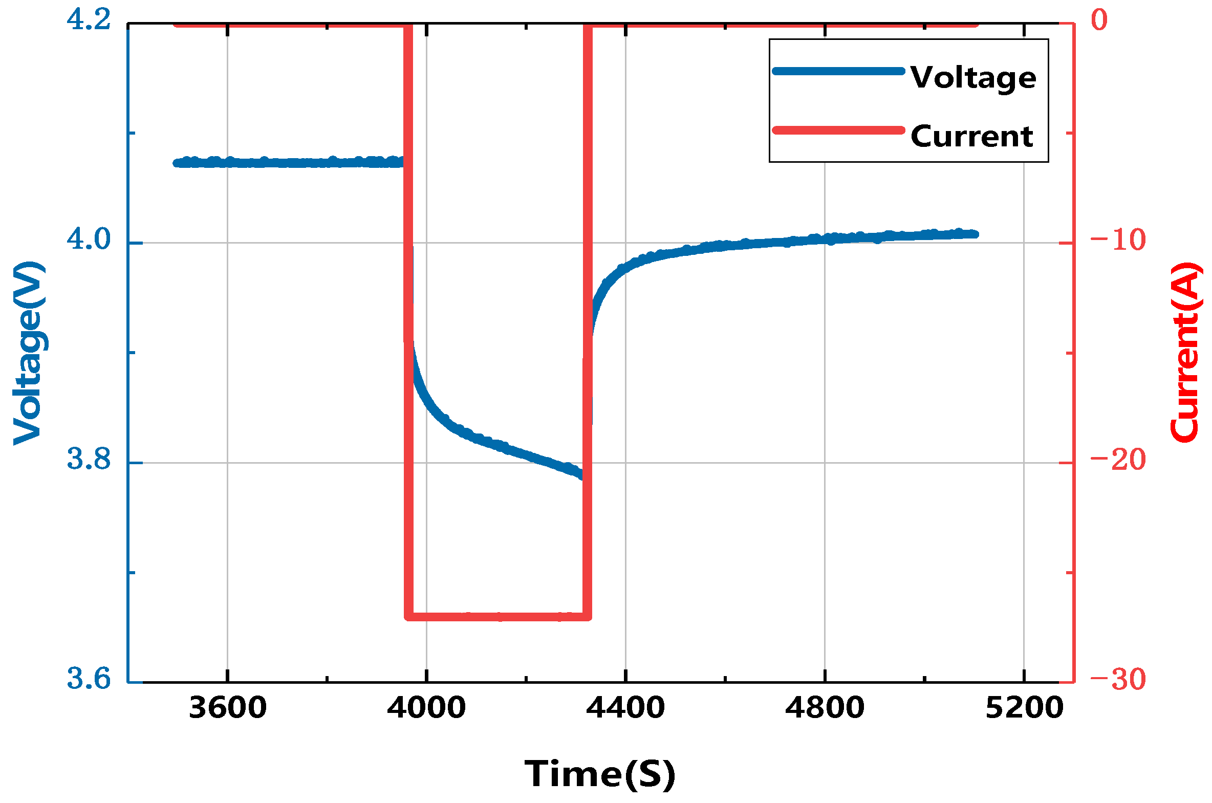
Firstly, an HPPC experiment was conducted to identify the offline parameters of the second order RC model. The results reveal that in the case of pulse-driven high current discharge, an instant drop in the terminal voltage of the battery occurs, as shown in Figure 2. Capacitance characteristics show that the capacitor is turned on in this process, and the bypass polarization resistance is short-circuited. Therefore, it must be the battery ohmic internal resistance that causes the instant voltage drop during pulse discharge. The voltage change curve in this process is shown in section AB of Figure 2 and was calculated as per Equation (15).

$$R_0=(U_0-U_c)/I$$

(15)

Upon canceling the pulse discharge current, the terminal voltage of the battery instantly increases. Since the voltage of the capacitor cannot suddenly change, the battery ohmic internal resistance remains the reason for the instant voltage rise when the battery is left standing still before the battery terminal voltage starts to rise slowly. This process is mainly due to the zero-input response of the RC link. The voltage change curve is shown in section DE of the figure. The battery output is calculated as per Equation (16).

$$U_{OC}(SOC)-U_t=U_1(0)e^{-\frac{\Delta t}{R_1{C}_1}}+U_2(0)e^{-\frac{\Delta t}{R_2{C}_2}}$$

(16)

In the equation, $U_1(0)$ and $U_2(0)$ are the voltage values of $R_1{C}_1$ and $R_2{C}_2$ at the moment after discharging is stopped. During pulse discharge, the two RC links can be regarded as zero-state responses. The voltage change curve in this process is presented in section BC of Figure 2, and the battery output in this process is calculated as per Equation (17). The parameters of the battery model can be calculated by substituting Equation (17) with the time constant calculated as per Equation (16).

$$U_{OC}(SOC)-U_t=I{R}_0+I{R}_1(1-e^{-\frac{\Delta t}{R_1{C}_1}})+I{R}_2(1-e^{-\frac{\Delta t}{R_2{C}_2}})$$

(17)

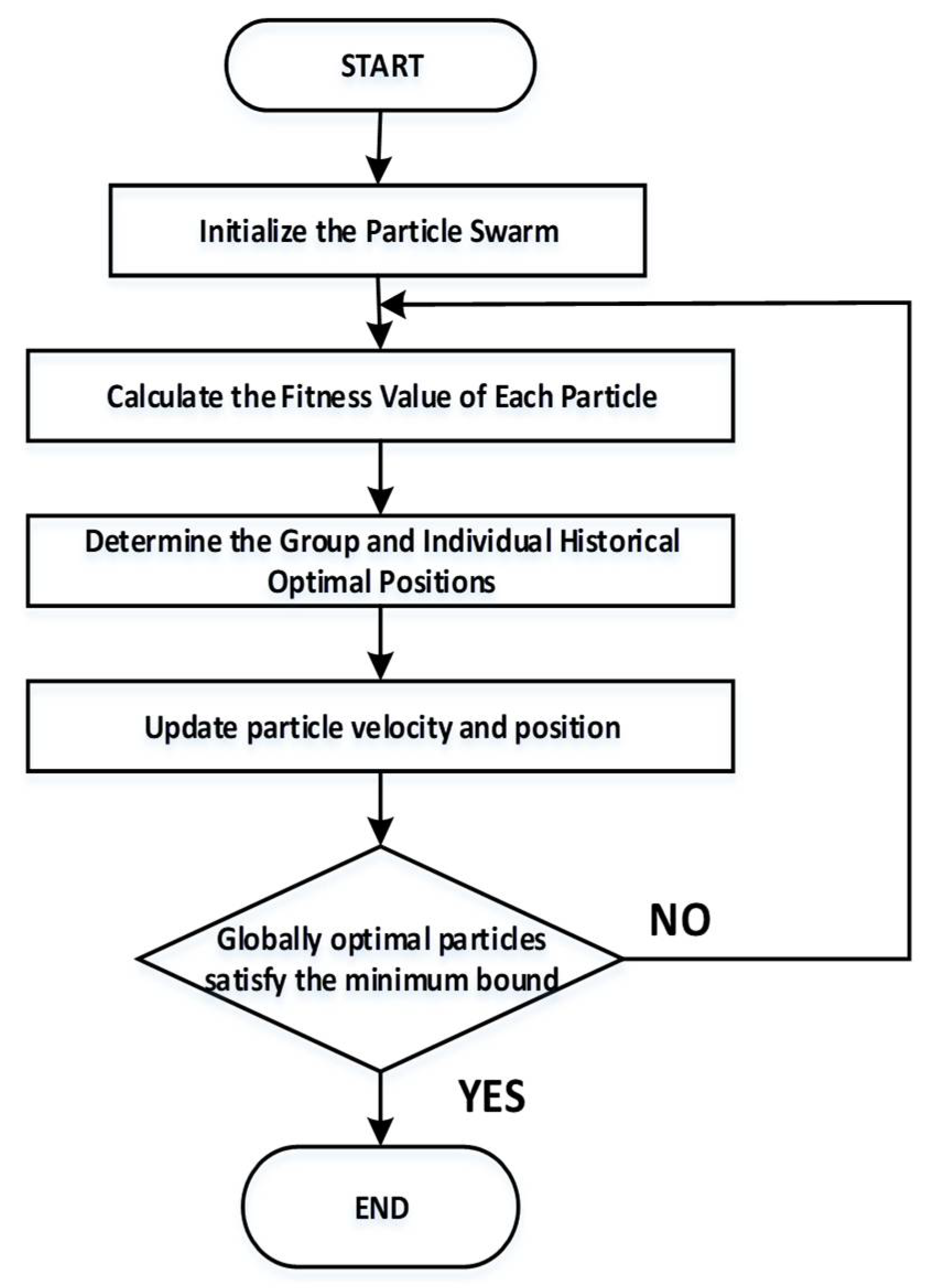
Next, a particle swarm optimization (PSO) algorithm was used to identify the parameters of the fractional order model. The parameters to be identified are $\theta =\left[\begin{array}{ccccccc}{R}_0& R_1& R_2& C_1& C_2& n_1& n_2\end{array}\right]$. Compared with the integer order model, there are two more capacitor orders. This algorithm is an immediate search algorithm based on group collaboration, which is easier to implement than the other algorithms. The fitness function is continuously optimized by updating the speed and position of particles in the space. When the fitness function is optimal, its position is also at the optimum. The fitness function is the minimum Euclidean norm between the terminal voltage $\widehat{U}(t)$ estimated by the fractional order model of the lithium battery, and the actual measured terminal voltage $U(t)$. The process of using the PSO algorithm to identify the capacitor order is illustrated in Figure 3.

$$J=\min {{\displaystyle {\int }_0^{+\infty }\Vert U(t)-\hat{U}(t)\Vert }}^{2}dt$$

(18)

4. Algorithm for Estimating the SOC of Lithium Battery

4.1. UKF Algorithm

The internal parameters of the lithium battery system are nonlinear and vary with time. The widely used expanded Kalman filter (EKF) algorithm is applicable to this kind of nonlinear system. The main idea involves carrying out a Taylor expansion of the state-space equation; therefore, it is necessary to calculate the Jacobian matrix if this algorithm is adopted. However, it suffers from a high computation burden. Meanwhile, the high second- and above orders are omitted in the Taylor expansion. This may cause an accumulation of errors in the estimation, resulting in inaccurate results.

In contrast, the UKF algorithm used for this kind of nonlinear system can approximate the probability density distribution of random variables instead of directly approximating the linearization of the nonlinear system. Compared with EKF, UKF can retain high order information, with an expected value accuracy and covariance reaching the third order approximation. Moreover, without the need for a differentiable model and calculation of the Jacobian matrix, UKF is easier to implement in hardware.

As the core of the UKF algorithm, the unscented transformation (UT) can be regarded as a Monte Carlo algorithm, whereby the approximations of the mean and covariance are obtained by constructing sigma points. UT is generally divided into the general, simple, and spherical types. If the model pursues fewer calculations, then the simple type should be used. If the model has a large number of dimensions, then it is necessary to use the spherical type, as the simple type may result in unstable values.

The UT can be explained mathematically as follows, whereby the second-order statistics are x and the nonlinear function is f:

$$y=f(x)\begin{array}{c}\end{array},\begin{array}{c}\end{array}{\mu }_x=E(x)\begin{array}{c}\end{array},\begin{array}{c}\end{array}{C}_x=Cov(x)$$

(19)

The UT can be expressed as follows:

$$\left[{\widehat{\mu }}_y,{\widehat{C}}_{yx},{\widehat{C}}_y\right]=UT(f,{\mu }_x,C_x)$$

(20)

Mathematically, UT can be equivalently expressed in an approximate integration format.

$${\displaystyle {\int }_{R^n}h(z){\phi }_x(z)dz}$$

(21)

In the equation, ${\phi }_x$ is the probability density function of $x$. When calculating the expected value $y$ of ${\widehat{\mu }}_y$, $h$ is equal to $f$ (i.e., $h=f$).

Currently, there are many types of UKF algorithms. In this paper, the following type is introduced:

Given that the nonlinear system model is

$$\{\begin{array}{c}{x}_k=f(x_{k-1},u_k)+w_k\\ y_k=h(x_k,u_k)+v_k\end{array}$$

(22)

(1) the initial value of the state observer is set.

$${\widehat{x}}_0^{+}=E(x_0),P_0^{+}=E[(x_0-{\widehat{x}}_0^{+}){(x_0-{\widehat{x}}_0^{+})}^T]$$

(23)

(2) the sigma point and the corresponding weight are calculated in a general UT format. Here, $P_{k-1}$ should be processed first, via the Cholesky decomposition.

$$P_{k-1}=S_{k-1}{(S_{k-1})}^T$$

(24)

$$\begin{gathered} \{\begin{array}{c}{w}_0^m=\frac{\lambda }{L+\lambda }\\ w_0^c=\frac{\lambda }{L+\lambda }+(1-{\alpha }^2+\beta )\\ w_i^m=w_i^c=\frac{\lambda }{2(L+\lambda )},i=1,\dots ,2L\end{array} \\ \{\begin{array}{c}{\widehat{x}}_{k-1}^{(0)}={\widehat{x}}_{k-1}^{+}\\ {\widehat{x}}_{k-1}^{(i)}={\widehat{x}}_{k-1}^{+}+(\sqrt{(L+\lambda )P_{k-1}}),i=1,\dots ,L\\ {\widehat{x}}_{k-1}^{(i)}={\widehat{x}}_{k-1}^{+}-(\sqrt{\left(L+\lambda \right)P_{k-1}}),i=L+1,\dots ,2L\end{array} \end{gathered}$$

(25)

(3) Time updating

$${\widehat{x}}_k^{(i)}=f({\widehat{x}}_{k-1}^{(i)},u_{k-1})$$

(26)

$${\widehat{x}}_k^{-}={\displaystyle {\sum }_{i=0}^{2L}{w}_i^m{\widehat{x}}_k^{(i)}}$$

(27)

$$P_k^{-}={\displaystyle {\sum }_{i=0}^{2L}{w}_i^c}({\widehat{x}}_k^{(i)}-{\widehat{x}}_k^{-}){({\widehat{x}}_k^{(i)}-{\widehat{x}}_k^{-})}^T+Q_k$$

(28)

(4) Measurement updating

$${\widehat{y}}_k^i=h({\widehat{x}}_k^{(i)},u_k)$$

(29)

$${\widehat{y}}_k={\displaystyle {\sum }_{i=0}^{2L}{w}_i^m}{\widehat{y}}_k^i$$

(30)

$$P_{yy,k}^{}={\displaystyle {\sum }_{i=0}^{2L}{w}_i^c}({\widehat{y}}_k^i-{\widehat{y}}_k){({\widehat{y}}_k^i-{\widehat{y}}_k)}^T+R_k$$

(31)

$$P_{xy,k}^{}={\displaystyle {\sum }_{i=0}^{2L}{w}_i^c}({\widehat{x}}_k^{(i)}-{\widehat{x}}_k^{-}){({\widehat{y}}_k^i-{\widehat{y}}_k)}^T$$

(32)

$$K_k=P_{xy,k}{(P_{yy,k}^{})}^{-1}$$

(33)

$${\widehat{x}}_k^{+}={\widehat{x}}_k^{-}+K_k(y_k-{\widehat{y}}_k)$$

(34)

$$P_k^{+}=P_k^{-}-K_k{P}_{yy,k}{K}_k^T$$

(35)

In summary, the following problems are encountered. Firstly, the covariance matrix $P_{k-1}$ must be positive definite and symmetric in order to conduct the Cholesky decomposition. However, in actual calculations, due to the loss of precision and the inversion link in the algorithm, the covariance matrix $P_{k-1}$ cannot constantly remain symmetric and positive definite. Furthermore, the more estimation parameters that are involved, the more likely it is to be non-positive definite, resulting in the failure of the algorithm. Secondly, in the UKF algorithm, the UT link is removed, and the remaining steps still fall within the standard KF framework. The UKF algorithm has the same requirements for system noise as the KF algorithm. Namely, the noise probability distribution is known, and it is considered that the state noises $w_k$ and $v_k$ are uncorrelated Gaussian white noises that conform to a normal distribution. However, the real noise is often colored noise, so the UKF algorithm itself still has certain limitations.

4.2. H-Infinity Filter (HIF) Algorithm

In the battery management system (BMS), the noise generated by a multitude of factors cannot be approximated to zero-mean uncorrelated white noise. Therefore, the use of UKF or KF alone can cause divergences or invalid estimation results. The colored noise of BMS is mainly caused by two factors. First is the noise generated by sensors. The main sensors in BMS include voltage, current, and temperature sensors. Due to the manufacturing process and design of circuitry, accuracy loss and electromagnetic interference are caused, and the noise generated cannot be regarded as zero-mean uncorrelated white noise. Second is the error of the noise covariance matrix. Sudden changes and a large range of change in electrical currents will affect the calculation of the mean noise value, and will further affect the calculation of the covariance matrix. It is also hard to determine the error generated at this time.

In order to filter out uncertain noise, the $H_{\infty }$ filter (HIF) algorithm is introduced here. Firstly, the cost function shown by Equation (36) is given below, where $y_k-{\widehat{y}}_k$ is the estimation error, $x_0-{\widehat{x}}_0$ is the error in the initial value, and $S_k$ represents the designer’s degree of interest in each state being evaluated.

$$J=\frac{{{\displaystyle \sum _{k=0}^{N-1}\Vert y_k-{\widehat{y}}_k\Vert }}^2{}_{S_k}}{{\Vert x_0-{\widehat{x}}_0\Vert }^2{}_{P_0^{-1}}+{\displaystyle \sum _{k=0}^{N-1}({\Vert w_k\Vert }_{Q_k^{-1}}^2+{\Vert v_k\Vert }_{R_k^{-1}}^2)}}$$

(36)

For any form of noise in the system, the purpose of the cost function is to calculate the accuracy of the estimated object, which is controlled within a certain range of proportions. According to game theory, in the KF algorithm, natural noise is idealized, and the noise that is treated as white noise is never changed. In contrast, in the HIF algorithm, natural noise is assumed as the worst condition.

The goal of this is to minimize the estimation error $y_k-{\widehat{y}}_k$, and to further obtain the smallest cost function, $J$. To facilitate the setting of the performance boundary to minimize cost function $J$, the following equations were used:

$$J<\frac{1}{\gamma }$$

(37)

After rearranging the above two equations, the following equation was obtained:

$$J=-\frac{1}{\theta }{\Vert x_0-{\widehat{x}}_0\Vert }^2{}_{P_0^{-1}}+{\displaystyle \sum _{k=0}^{N-1}\left[{\Vert x_k-{\widehat{x}}_0\Vert }^2{}_{\stackrel{-}{S_k}}-\frac{1}{\theta }({\Vert w_k\Vert }^2{}_{Q_k^{-1}}+{\Vert y_k-C_k{x}_k-D_k{u}_k\Vert }^2{}_{R_k^{-1}})\right]}$$

(38)

Based on the above equation, the minimization of the cost function was transformed into the following minimax equation:

$$J=\underset{\stackrel{\wedge }{x_k}}{\min }\underset{\stackrel{}{w_k,z_k,x_0}}{\max }\begin{array}{c}J\end{array}$$

(39)

The goal of the calculation results was to make the cost function $J$ lower than $1/\gamma$. The following is a brief introduction to the iteration process of the HIF algorithm:

(1) Initialization:

$$x_0,P_0,S_0,Q_0,R_0$$

(40)

(2) Updating the prior states estimation:

$${\widehat{x}}_{k+1}^{-}=f({\widehat{x}}_k^{+},u_k)$$

(41)

(3) Updating the prior states error covariance:

$$P_{k+1}^{-}=A_{1,k}^{}{P}_k^{+}{A}_{1,k}^T+Q_k$$

(42)

(4) Updating the symmetric positive definite matrix:

$${\stackrel{-}{S}}_k=L_k^T{S}_k{L}_k$$

(43)

Correction of measured value.

(5) Updating gain matrix:

$$K_{k+1}=A_{k+1}{P}_{k+1}^{-}{(I-1/\gamma {\stackrel{-}{S}}_k{P}_{k+1}^{-}+C_{k+1}^T{R}_{k+1}^{-1}{C}_{k+1}{P}_{k+1}^{-})}^{-1}{C}_{k+1}^T{R}_{k+1}^{-1}$$

(44)

(6) Updating the posteriori state value:

$${\widehat{x}}_{k+1}^{+}={\widehat{x}}_{k+1}^{-}+K_{k+1}(z_{k+1}-h({\widehat{x}}_{k+1}^{-},u_{k+1}))$$

(45)

(7) Updating the posteriori variance:

$$P_{k+1}^{+}=A_{1,k}{P}_{k+1}^{-}{(I-1/\gamma S_k{P}_{k+1}^{-}+C_k^T{R}_k^T{C}_k^{}{P}_{k+1}^{-})}^{-1}{A}_{1,k}^T+Q_k$$

(46)

As discovered from the above process, it is possible to obtain the relationship between the converted HIF and KF algorithms by changing the limiting factor, $\gamma$. When $\gamma =0$, the HIF algorithm becomes the KF algorithm. In other words, the KF algorithm is a special iteration of the HIF algorithm with an infinite performance boundary. Moreover, there are some limitations in the HIF algorithm. (1) In the HIF algorithm, there are no specific measures for the linearization of the nonlinear system, and (2) although colored noise can be filtered out in the HIF algorithm, the state noise variance and measurement noise variance matrices should still be assumed in advance. The assumed value also has a direct effect on the final estimation result, resulting in amplified or divergent errors.

4.3. Fractional Order Model-Based Unscented Kalman Filter and H-Infinity Filter (FOUHIF) Estimation Algorithm

The internal chemical mechanism of lithium batteries is complex, and the parameters have an extremely strong nonlinearity relationship. In addition, the noise probability distribution of lithium batteries is unknown under different working conditions and electrical currents. Based on the above-mentioned problems of lithium batteries and the analysis formed in Chapter 4, a fractional order model-based unscented Kalman filter and H-infinity filter (FOUHIF) estimation algorithm was proposed, with the UKF algorithm as the main framework, and its UT change can improve estimation accuracy and speed. In the FOUHIF algorithm, an HIF algorithm was incorporated to solve the problem where all noise had to be assumed to be white noise in the UKF algorithm. Colored noise was filtered out by minimizing the cost function. Meanwhile, in order to improve estimation accuracy, the FOUHIF algorithm was combined with the lithium battery fractional order model. Namely, the expected value and error covariance matrix of the priori state estimation value were transformed into a fractional order format. Furthermore, some issues with the two algorithms were also improved: firstly, the singular value decomposition of the covariance matrix $P_k$ was carried out to solve the original problem of an ill-conditioned matrix being generated during the Cholesky decomposition. Secondly, a self-adaption method was used to solve the problem of the uncertain initial values of the state noise covariance and the measurement noise covariance matrices.

If the SVD method is used, the decomposed matrix is neither required to be positive definite nor required to be a square matrix. This means that any matrix is suitable for SVD decomposition. Assuming that the matrix $A$ is an $m\times n$ matrix, the SVD of matrix $A$ is defined as:

$$\mathbf{A}=US{V}^T\iff \left[U,S,V\right]=SVD(\mathbf{A})$$

(47)

$$S={\left[\begin{array}{cc}{\displaystyle \sum }& 0\\ 0& 0\end{array}\right]}_{m\times n},{\displaystyle \sum }=diag({\sigma }_1,{\sigma }_2,\dots ,{\sigma }_n)$$

In the above two equations, matrices $U$ and $V$ are orthogonal matrices; the column vector $u_i$ of $U$ is the eigenvector of matrix $A{A}^T$; the column vector $v_i$ of $V$ is the eigenvector of matrix $A^{T}A$; ${\sigma }_i$ is the singular value; and ${\sigma }_i^2$ is the eigenvalue of the matrix $A{A}^T$.

The detailed steps of the FOUHIF algorithm are as follows:

(1) Initialization:

$${\widehat{x}}_0^{+}=E(x_0),P_0^{+}=E[(x_0-{\widehat{x}}_0^{+}){(x_0-{\widehat{x}}_0^{+})}^T]$$

(48)

(2) Performing SVD on $P_k$,and calculating the sampling points and corresponding weight values:

$$\left[\begin{array}{ccc}u& S& v\end{array}\right]=SVD(P_k)$$

(49)

$$\{\begin{array}{c}{w}_0^m=\frac{\lambda }{L+\lambda }\\ w_0^c=\frac{\lambda }{L+\lambda }+(1-{\alpha }^2+\beta )\\ w_i^m=w_i^c=\frac{\lambda }{2(L+\lambda )},i=1,\dots ,2L\end{array}$$

(50)

$$\{\begin{array}{c}{\widehat{x}}_{k-1}^{(0)}={\widehat{x}}_{k-1}^{+}\\ {\widehat{x}}_{k-1}^{(i)}={\widehat{x}}_{k-1}^{+}+(\sqrt{(L+\lambda )S}),i=1,\dots ,L\\ {\widehat{x}}_{k-1}^{(i)}={\widehat{x}}_{k-1}^{+}-(\sqrt{\left(L+\lambda \right)S}),i=L+1,\dots ,2L\end{array}$$

(51)

(3) Update time: The state variables ${\widehat{x}}_1^{+},\dots ,{\widehat{x}}_{k-1}^{+}$ are required to calculate the expected value and the error covariance matrix of the priori state estimation variable; Equation (9) is the nonlinear state transfer function (52), and the maximum difference between the fractional order UKF and the integer order UKF is shown in Equations (52)–(54). The detailed derivation process can be found in Reference [22].

$${\widehat{x}}_k^{(i)}=f({\widehat{x}}_{k-1}^{(i)},u_{k-1})$$

(52)

$${\widehat{x}}_k^{-}=E\left(f({\widehat{x}}_{k-1}^{(i)},u_{k-1})-{\displaystyle \sum _{j=1}^k{K}_j{\widehat{x}}_{k-j}^{+}}\right)={\displaystyle \sum _{i=0}^{2L}{w}_i^m}{\widehat{x}}_k^{(i)}-{\displaystyle \sum _{j=1}^k{K}_j}{\widehat{x}}_{k-j}^{+}$$

(53)

$$\begin{array}{l}{P}_k^{-}={\displaystyle \sum _{i=0}^{2L}{w}_i^c}({\widehat{x}}_k^{(i)}-{\displaystyle \sum _{i=0}^{2L}{w}_i^m{\widehat{x}}_k^{(i)}})({\widehat{x}}_k^{(i)}-{\displaystyle \sum _{i=0}^{2L}{w}_i^m{\widehat{x}}_k^{(i)}}{)}^T\\ \begin{array}{cc}& \end{array}\hspace{1em}+{\displaystyle \sum _{j=1}^k(K_j{\widehat{x}}_{k-j}^{+}}{\displaystyle \sum _{i=0}^{2n}{w}_i^{(c)}({\widehat{x}}_k^{(i)}}-{\displaystyle \sum _{i=0}^{2n}{w}_i^{(m)}{\widehat{x}}_k^{(i)}}{)}^T\\ \begin{array}{cc}& \end{array}\hspace{1em}+{\displaystyle \sum _{j=1}^K{\displaystyle \sum _{i=0}^{2n}{w}_i^{(c)}({\widehat{x}}_k^{(i)}-{\displaystyle \sum _{i=0}^{2n}{w}_i^{(m)}{\widehat{x}}_k^{(i)}})(}}{\widehat{x}}_{k-j}^{+}{)}^T(K_j{)}^T\\ \begin{array}{cc}& \end{array}\hspace{1em}+{\displaystyle \sum _{j=1}^k{K}_j{\widehat{x}}_{k-j}^{+}({\widehat{x}}_{k-j}^{+}{)}^T{(K_j)}^T+Q_k}\end{array}$$

(54)

(4) Updating the measurements and calculating the predicted value ${\widehat{y}}_k$ of the output and the covariance matrix $P_{yy,k}$ and P_xy,k, where the nonlinear measurement function is expressed by Equation (9):

$${\widehat{y}}_k^i=h({\widehat{x}}_k^{(i)},u_k)$$

(55)

$${\widehat{y}}_k={\displaystyle \sum _{i=0}^{2L}{w}_i^m{\widehat{y}}_k^i}$$

(56)

$$P_{yy,k}^{}={\displaystyle {\sum }_{i=0}^{2L}{w}_i^c}({\widehat{y}}_k^i-{\widehat{y}}_k){({\widehat{y}}_k^i-{\widehat{y}}_k)}^T+R_k$$

(57)

$$P_{xy,k}^{}={\displaystyle {\sum }_{i=0}^{2L}{w}_i^c}({\widehat{x}}_k^{(i)}-{\widehat{x}}_k^{-}){({\widehat{y}}_k^i-{\widehat{y}}_k)}^T$$

(58)

(5) The above steps are identical to those of the fractional order UKF algorithm. Afterwards, the posteriori state estimation value was corrected:

$$K_k=P_{xy,k}{(P_{yy,k}^{})}^{-1}$$

(59)

$${\widehat{x}}_k^{+}={\widehat{x}}_k^{-}+K_k(y_k-{\widehat{y}}_k)$$

(60)

$$P_k^{+}=P_k^{-}-\left[\begin{array}{cc}{P}_{xy,k}& P_k^{-}\end{array}\right]R_{e,k}^{-}{\left[\begin{array}{cc}{P}_{xy,k}& P_k^{-}\end{array}\right]}^T$$

(61)

$$R_{e,k}=\left[\begin{array}{cc}R+P_{yy,k}& {(P_{xy,k})}^T\\ P_{xy,k}& {\gamma }^{2}I+P_k^{-}\end{array}\right]$$

(62)

The specific derivation processes of Equations (61) and (62) can be seen in Reference [18]. In Reference [18], the range of ${\gamma }^2$ based on the integer order battery model was derived from the above two equations. In this paper, the range of ${\gamma }^2$ based on the fractional order battery model was derived from the above two equations.

According to the characteristics of the lithium battery state equation, the following equation was obtained by substituting Equation (54) into Equation (61).

$$P_k^{+}=P_k^{-}-{\gamma }^2{P}_{xy,k}^{}{P}_{xy,k}^{}-P_k^{-}R{P}_k^{-}$$

(63)

By carrying out an inversion calculation on both sides of the equation and simplifying it, the following equation was obtained:

$${(P_k^{+})}^{-1}={(P_k^{-})}^{-1}-{\gamma }^{-2}I-{(P_k^{-})}^{-1}{P}_{xy,k}^{}{R}^{-1}{\left[{(P_k^{-})}^{-1}{P}_{xy,k}^{}\right]}^T$$

(64)

Since $P_k^{+}$ is symmetrical and positive definite, the above equation should be greater than 0. Hence:

$${(P_k^{-})}^{-1}-{(P_k^{-})}^{-1}{P}_{xy,k}^{}{R}^{-1}{\left[{(P_k^{-})}^{-1}{P}_{xy,k}^{}\right]}^T>{\gamma }^{-2}I$$

(65)

${\gamma }^{-2}$ can be regarded as the eigenvalue of the left side of the above equation, so:

$${\gamma }^2>\alpha \max \{eig{({(P_k^{-})}^{-1}-{(P_k^{-})}^{-1}{P}_{xy,k}^{}{R}^{-1}{\left[{(P_k^{-})}^{-1}{P}_{xy,k}^{}\right]}^T)}^{-1}\}$$

(66)

${\gamma }^2$ takes the largest eigenvalue, which can be calculated by the following equation:

$${\gamma }^2=\beta \max \{eig{({(P_k^{-})}^{-1}-{(P_k^{-})}^{-1}{P}_{xy,k}^{}{R}^{-1}{\left[{(P_k^{-})}^{-1}{P}_{xy,k}^{})\right]}^T)}^{-1}\}$$

(67)

Thereby, Equations (61), (62), and (67) are applicable to both the integer order model and the fractional order model. ${\gamma }^2$ has the same function as the cost function in the HIF algorithm. By adjusting ${\gamma }^2$, it is possible to improve the robustness to colored noise and correct the ill-conditioned matrix that is encountered when calculating the covariance matrix. When ${\gamma }^2$ tends to infinity, the FOUHF algorithm is equivalent to the FOUKF algorithm, where $\beta$ is not less than 1.

Next, a self-adaption algorithm was used to correct the noise covariance matrix $Q$ and matrix $R$.

$$\Delta U_k=U_k-[k_0+R_0{i}_k+\frac{k_1}{z_k}-k_2{z}_k-k_3\ln (z_k)-k_4\ln (1-z_k)]$$

(68)

$$F_k\approx \frac{{\displaystyle \sum _{n=k-L+1}^k\Delta U_n\Delta U_n^T}}{L}$$

(69)

$$Q_k=K_k{F}_k{K}_k^T$$

(70)

$$R_k=F_k+{\displaystyle \sum _{i=0}^{2n_x}{w}_i^c(\stackrel{\wedge }{y_k^i}}-\widehat{U_k+\Delta U}){(\stackrel{\wedge }{y_k^i}-U_k+\Delta U)}^T$$

(71)

where $\Delta U$ is the terminal voltage error value output used by the model at time $k$, and $F_k$ is the approximate value of the terminal voltage error covariance used by the model at time $k$.

5. Experiment

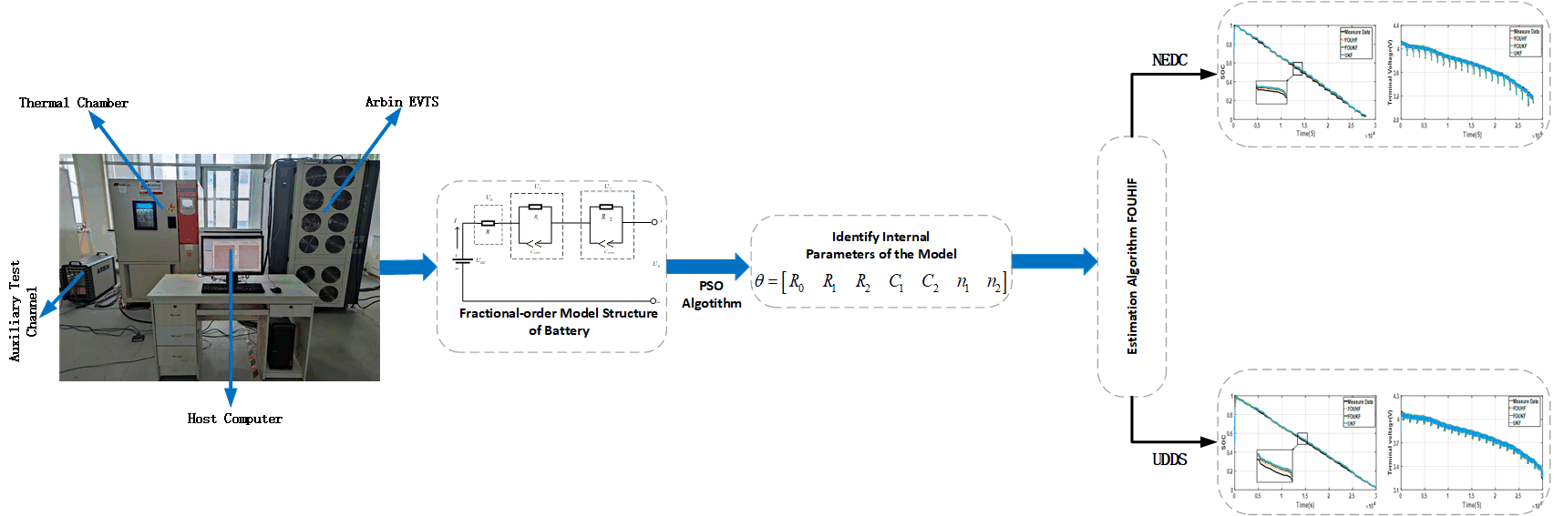
5.1. Experiment Platform

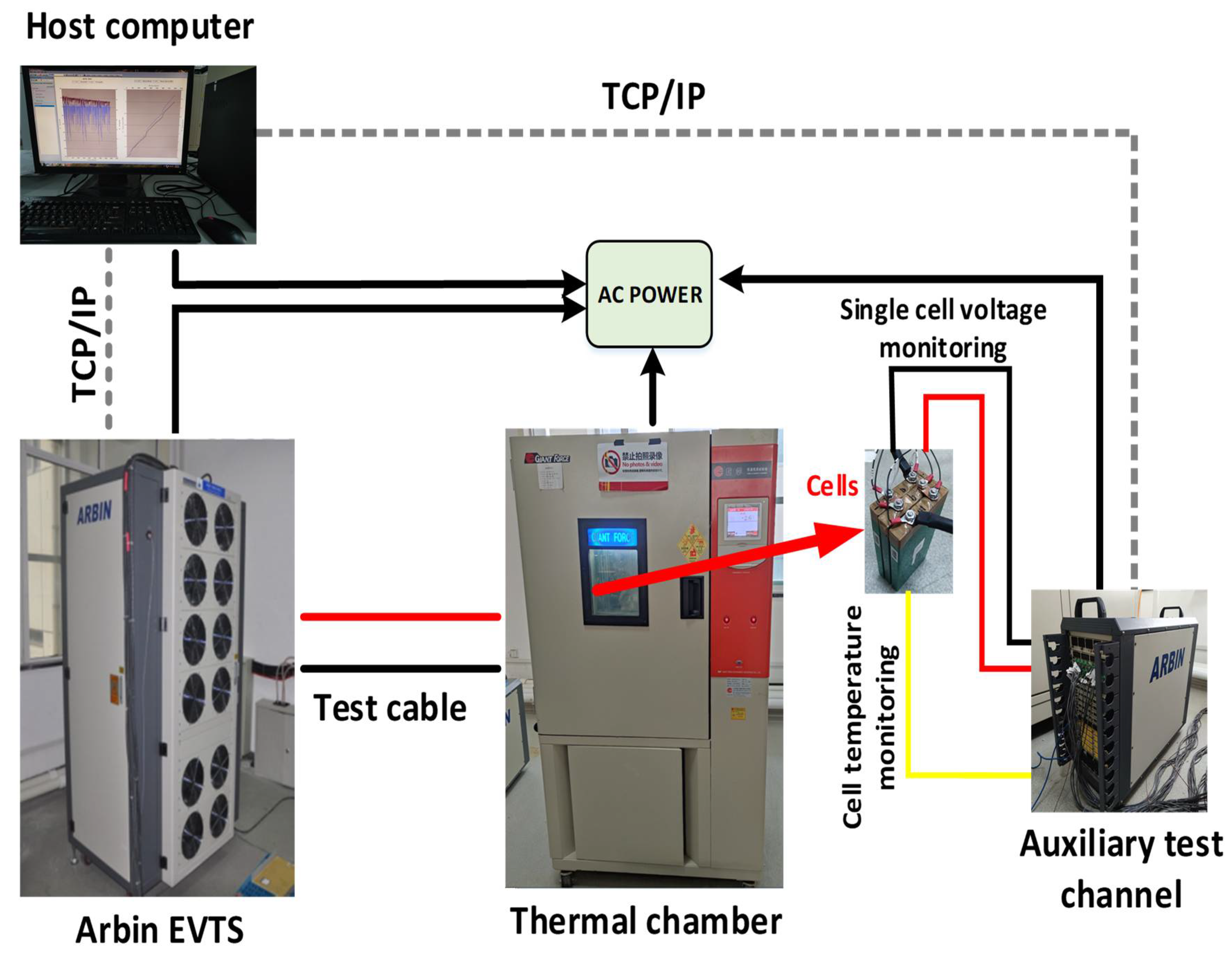
In order to verify the effectiveness of the algorithm proposed in this paper, a lithium battery test platform set was established for this experiment. This platform mainly consisted of the following components: (1) an electric vehicle battery test system (EVTS) produced by Arbin (USA) with a measurement accuracy of $\pm 0.1\%FSR$, (2) a constant temperature and moisture testing machine produced by Giant Force Company for controlling the ambient temperature of the lithium battery, (3) an upper computer for collecting the lithium battery parameters, (4) a battery pack composed of three ternary lithium batteries. The specific parameters of the battery pack are shown in

Table 1. Battery parameters.

Name of Parameter	Value
Nominal capacity	27 Ah
Nominal voltage	3.7 V
Charging cut-off voltage	4.2 V
Discharging cut-off voltage	2.75 V
Size	17 × 90 × 200 mm

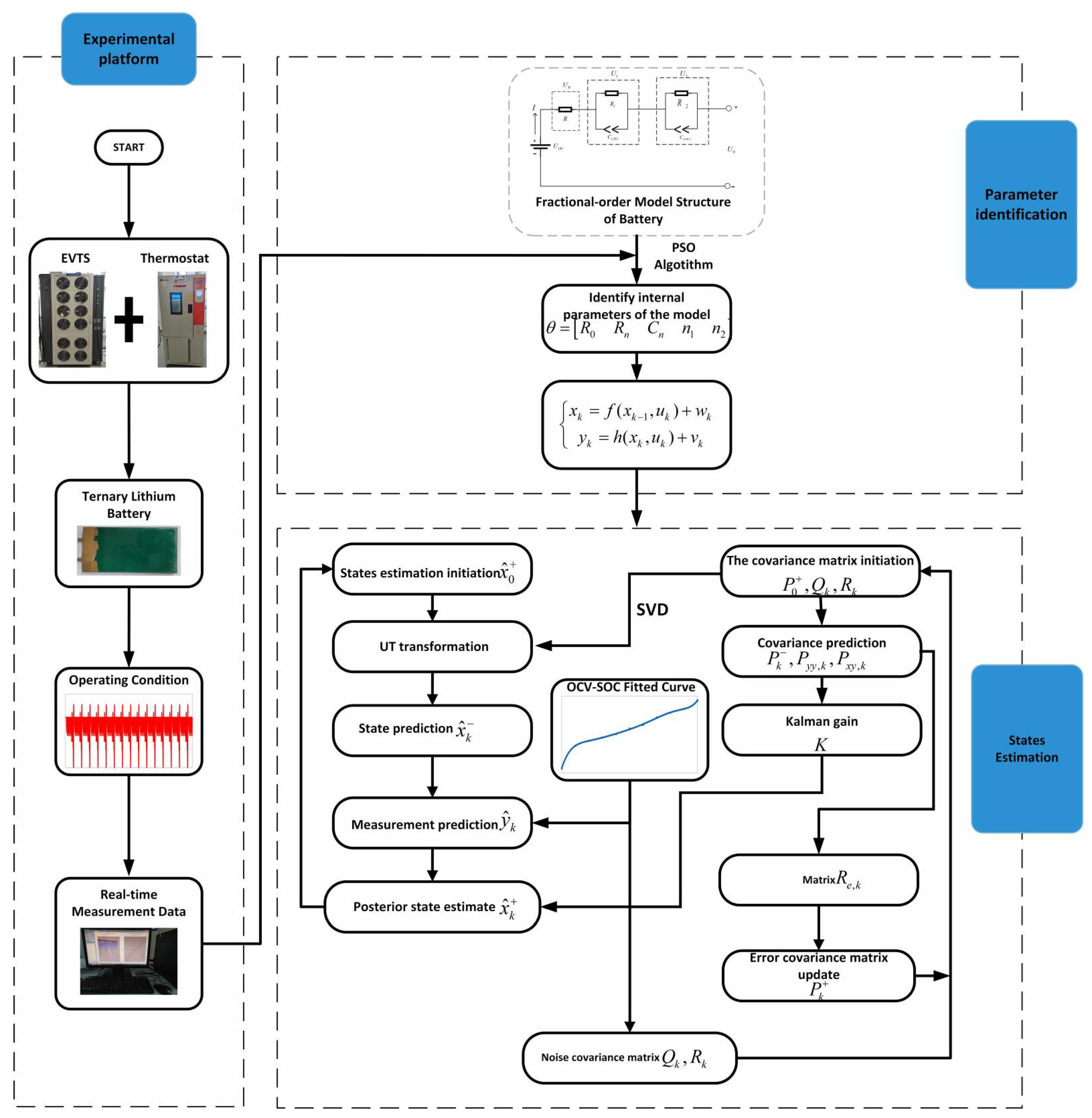
, and the physical diagram of the experimental platform is shown in Figure 4. Figure 5 shows the flow of the PSO identification algorithm and the FOUHIF algorithm.

5.2. Identification of the Parameters of Lithium Battery Model

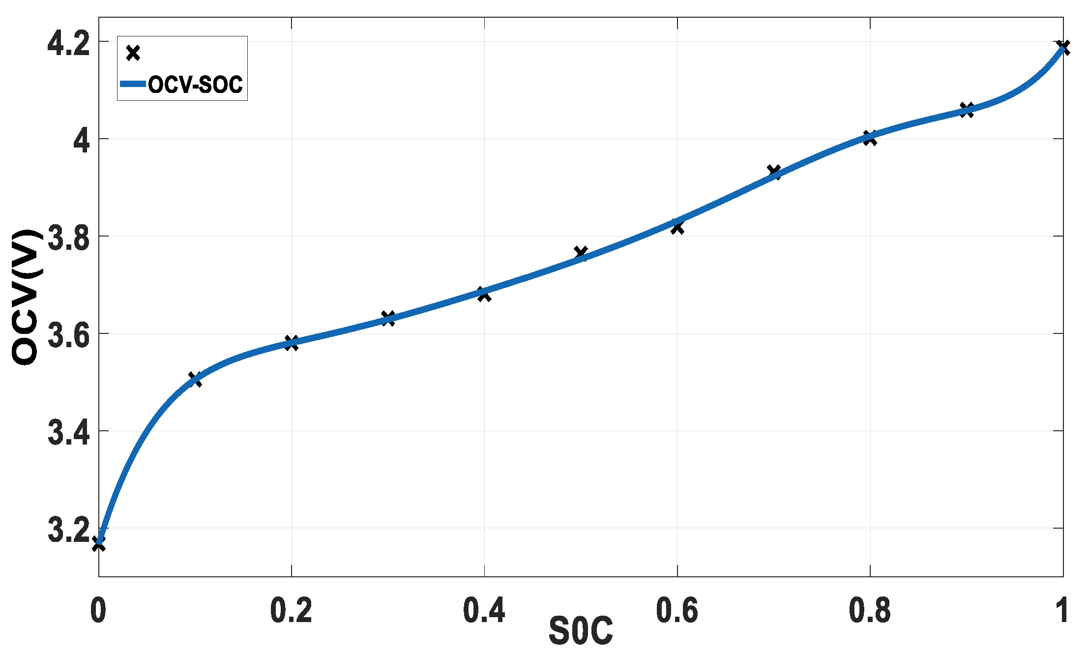
The function relationship between OCV and SOC was calculated before carrying out the parameter identification and SOC estimation. The experimental temperature was set at 25 °C to measure the charge and discharge curves of the lithium battery and to calculate the mean value. Then, by fitting based on Equation (14), the OCV–SOC curve of the battery was obtained, as shown in Figure 6.

The accuracy of the identified internal parameters of the equivalent circuit model has a direct effect on the estimation of the SOC. Meanwhile, in order to prove the superiority of the fractional order model, the HPPC experiment method and the PSO algorithm introduced in Chapter 3 were taken to identify the internal parameters of the second order RC and fractional order models. Then, a comparison was made on the operating effects of the parameters identified by the two methods under the working conditions of HPPC.

Table 2. Identification results of battery parameters.

	${\mathit{R}}_0(\mathit{m}\mathbf{\Omega })$	${\mathit{R}}_1(\mathit{m}\mathbf{\Omega })$	${\mathit{R}}_2(\mathit{m}\mathbf{\Omega })$	${\mathit{C}}_1(\mathit{F})$	${\mathit{C}}_2(\mathit{F})$	${\mathit{n}}_1$	${\mathit{n}}_2$
Two-order	6	2.6	3.5	12,470	26,981	-	-
Fractional-order	6	1.7	1.2	17,283	60,181	0.91	0.82

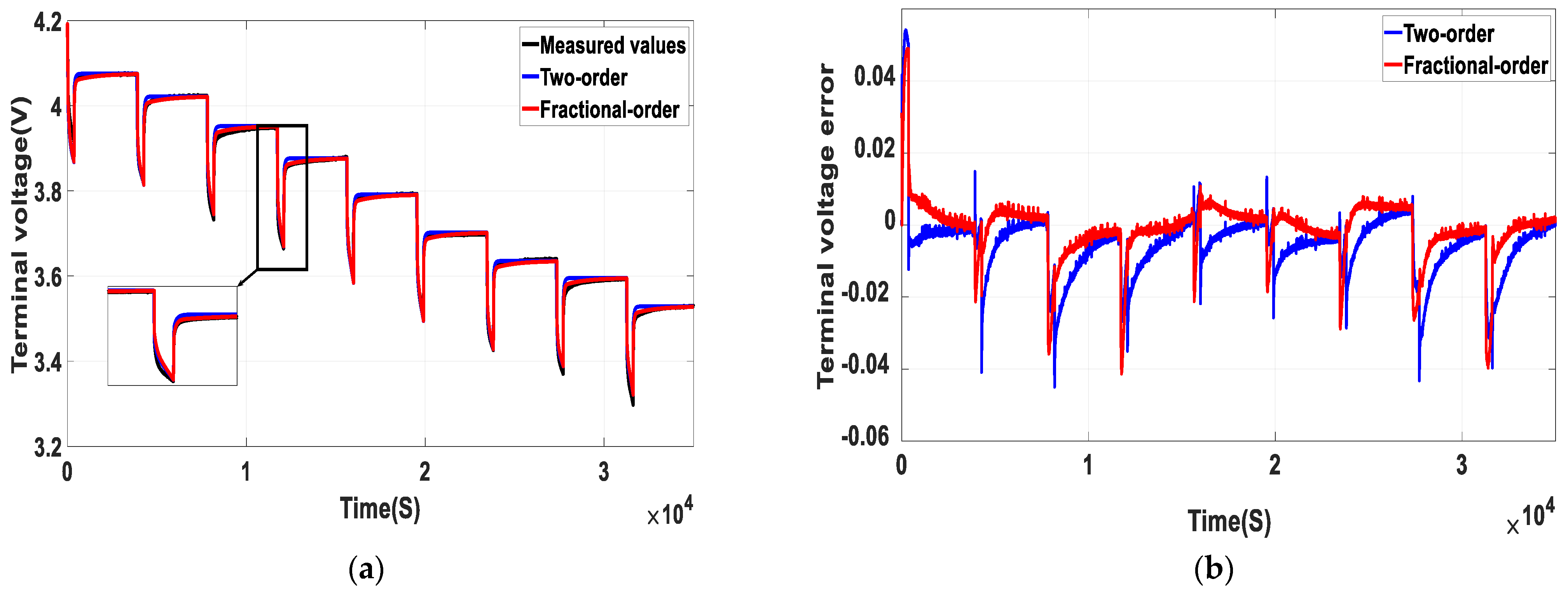
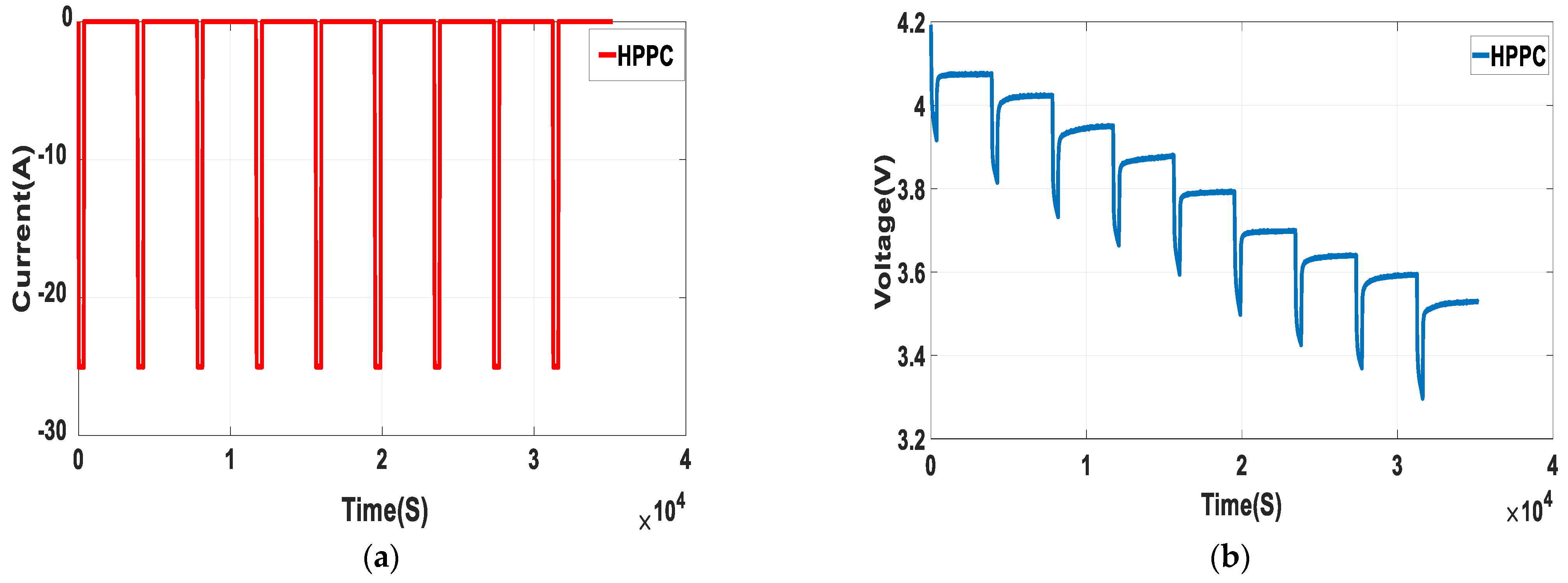
illustrates the results identified by the two types of models. It was revealed that the fractional order model and the integer order model have fairly different parameters; the two capacitor orders in the fractional order model were 0.91 and 0.82 respectively, which is consistent with the conclusion made in reference [23]. Namely, the lower the loss, the closer the order is to 1. Figure 7a,b demonstrate the current and voltage curves under the working conditions of HPPC, and Figure 8a presents a comparison between the actual value of the terminal voltage and the estimated value of the terminal voltage, which were obtained from the fractional order and integer order RC models. The graph in Figure 8b represents the error in the terminal voltage estimated by the two types of models. As can be seen in Figure 8 and

Table 3. Statistical data of terminal voltages under HPPC cycles.

	RMSE(%)	MAE(%)
Two-order	2.28	1.66
Fractional-order	1.75	1.39

, compared with the integer order model, the depiction of lithium batteries by the fractional order model is more accurate, because the mean absolute error (MAE) was reduced from 1.66% to 1.39%. Meanwhile, the stability index (RSME) of the estimated terminal voltage decreased from 2.28% to 1.75%.

It can be seen from the identification results that the parameters of the fractional order equivalent circuit model are significantly different from those of the integer order equivalent circuit model. This is especially the case for the capacitance value. The main reason for this is that the integer order equivalent circuit model is too simple, and only reflects the ohmic, concentration, and electrochemical polarization in the lithium battery. Meanwhile, the fractional order model not only reflects the three chemical reactions, but also reflects the double electric layer effect, and the transfer reaction between the electrolyte and solid phase interface.

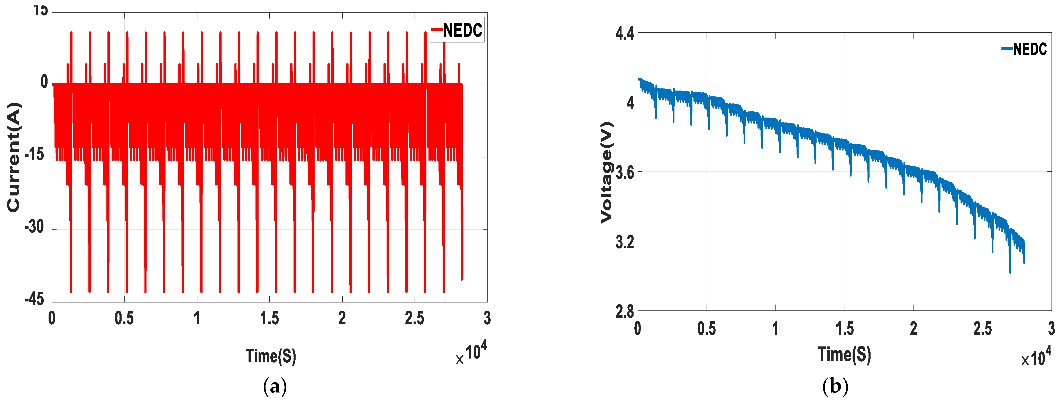
5.3. Verification of SOC under the Working Condition of NEDC

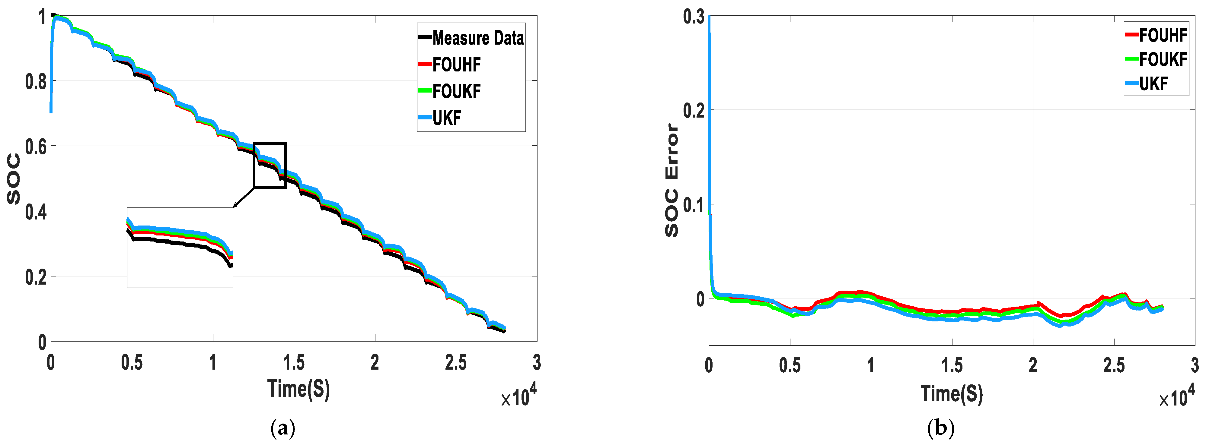
In order to verify the accuracy and robustness of the algorithm proposed in this research, the working conditions for the complicated New European Driving Cycle (NEDC) were selected when running tests on the battery. Under these working conditions, the electric current fluctuated greatly, making it more suitable for testing the performance of the algorithm at filtering colored noise. In the meantime, considering that the initial value of the SOC cannot be determined in actual engineering applications, it was necessary to evaluate whether or not the SOC could be quickly corrected in the algorithm when the initial value of the SOC was inaccurate. Therefore, in this research, the initial value of the SOC was set at 70%, the initial error was artificially set at 30%, and the memory length of the fractional order model was set at 70.

Figure 9a,b show the current and voltage under the NEDC working conditions. Figure 10a illustrates the SOC values of the battery estimated by FOUHIF, FOUKF, and the UKF algorithm, respectively, under the NEDC working conditions. Figure 10b presents the errors in SOC estimated by the three algorithms. As can be observed in these figures, FOUHIF had the highest robustness and greatest estimation effect; the UKF algorithm had the worst estimation effect under these working conditions; and in the FOUHIF algorithm, the root-mean-square error (RSME), mean absolute error (MAE), and maximum absolute error (ME) were reduced to 0.94, 0.78, and 1.86% respectively. Furthermore, the maximum error in the estimated SOC value appears at the 13,686th second. This reflects an improvement in SOC estimation accuracy and improved robustness. Figure 10c demonstrates the terminal voltage values estimated by the three algorithms. The voltage predicted by the three algorithms can track the measured value quickly. However, the maximum absolute error in the terminal voltage predicted by the FOUHIF algorithm was only 5.29 mV. the specific results are shown in Figure 10d.

Table 4. Statistical data of SOC under NEDC cycles.

	RSME (%)	MAE (%)	ME (%)
FOUHIF	0.94	0.78	1.86
FOUKF	1.29	1.10	2.53
UKF	1.57	1.33	2.91

shows the SOC estimation errors of the three algorithms under the NEDC condition.

The main factors that significantly affected the measurement uncertainty of the lithium battery SOC are the uncertainty caused by the measurement repeatability of the terminal voltage and the measurement error of the battery cycle test equipment itself, as evaluated by class A and class B, respectively. Under the NEDC working conditions, the uncertainty analysis of the three estimation methods was conducted to select the time period when the battery was standing, ranging from 11,711 to 11,741 s. First, the functional relationship between the measured voltage $U_{OCV}$ of battery and the estimated SOC value was fitted, thus obtaining Formula (72). Second, Formula (73) was used to calculate the standard uncertainties $u_x$ of the directly measured value $U_{OCV}$. Formula (74) is the propagation formula between the directly measured voltage $U_{OCV}$ and the indirectly measured SOC value. Third, the propagation formula was used to calculate the standard uncertainties of the indirectly measured SOC value. Therefore, the uncertainty components of the UKF, FOUKF and FOUHIF estimation methods caused by repeated measurements were $6.0\times {10}^{-4}$, $9.8\times {10}^{-5}$ and $5.3\times {10}^{-6}$, respectively. Fourth, Formula (75) was used to calculate the uncertainties caused by the error of the instruments where, $\Delta x$ is the limit error. It was assumed that the error was normally distributed and that $k=\sqrt{3}$. Therefore, the uncertainties caused by equipment indication errors were $5.7\times {10}^{-3}$, $4.9\times {10}^{-3}$, and $4.1\times {10}^{-4}$, respectively. Finally, Formula (76) was used to calculate the combined standard uncertainties of the estimated SOC value; the standard uncertainties of the three methods were $5.8\times {10}^{-3}$, $4.9\times {10}^{-3}$ and $4.1\times {10}^{-4}$. For the selected measurement time interval, the measurement results of the three measurement methods were $0.605\pm 0.0058$, $0.602\pm 0.0049$ and $0.600\pm 0.00041$, respectively. Therefore, in terms of uncertainty, the FOUHIF algorithm had the highest reliability when analyzing the three measurement methods.

$$SOC=f(U_{ocv})$$

(72)

$$u_x={\left(\frac{{\displaystyle \sum {(x_u-\stackrel{-}{x})}^2}}{n-1}\right)}^{1/2}$$

(73)

$$u_{y,1}=\left|\frac{\partial SOC}{\partial U_{OCV}}\right|u_x$$

(74)

$$u_{y,2}=\frac{\Delta x}{k}$$

(75)

$$u_{\mathrm{c}}=\sqrt{u_{y,1}^2+u_{y,2}^2}$$

(76)

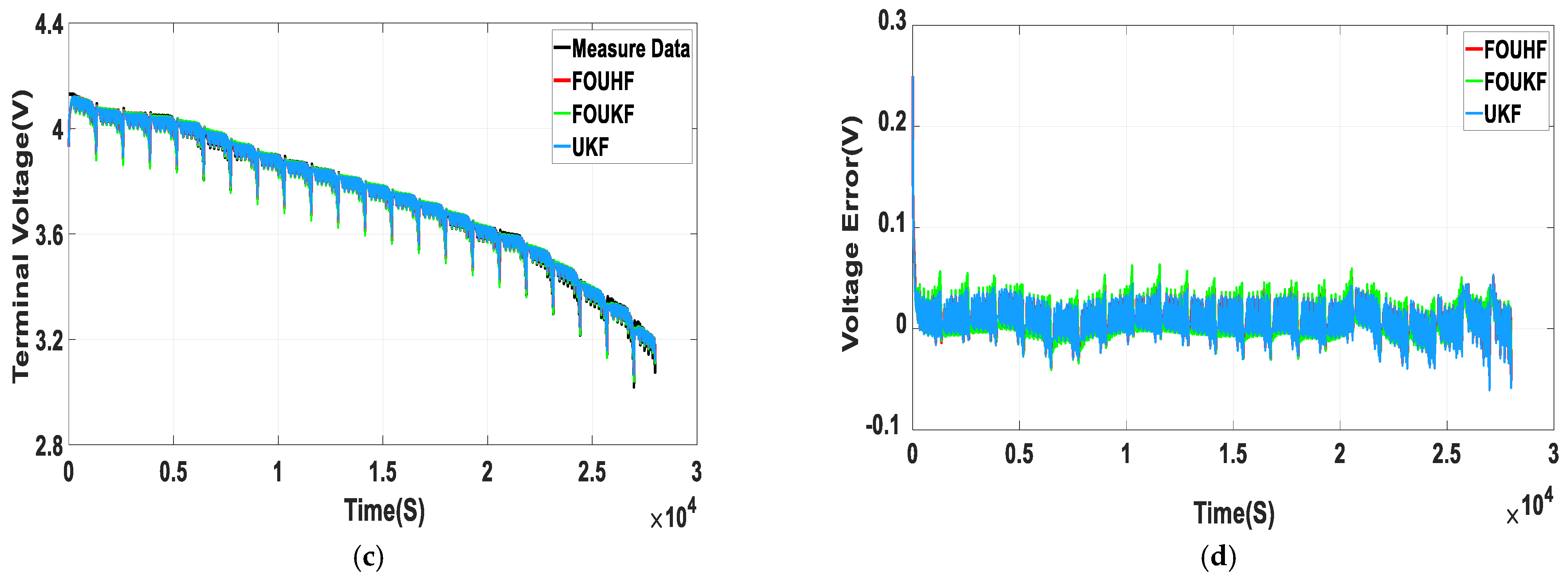
5.4. Verification of SOC under the Working Condition of UDDS

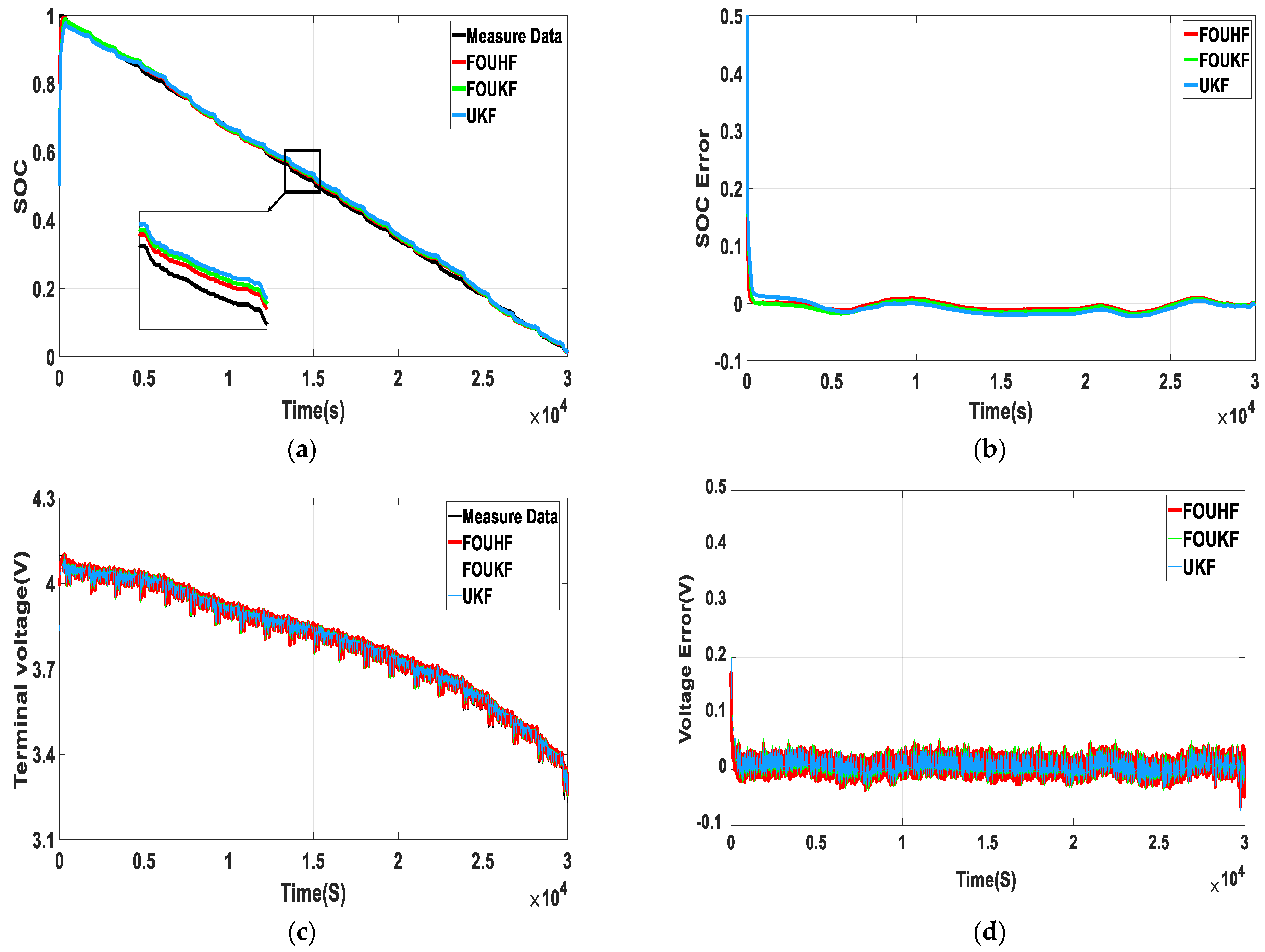
In order to further verify the robustness and universality of the FOUHIF algorithm, lithium batteries were also tested under UDDS working conditions, and an estimation was made on the SOC of the battery by the aforementioned three algorithms. The initial value of SOC was set as 0.5, and the initial error was set as 50%.

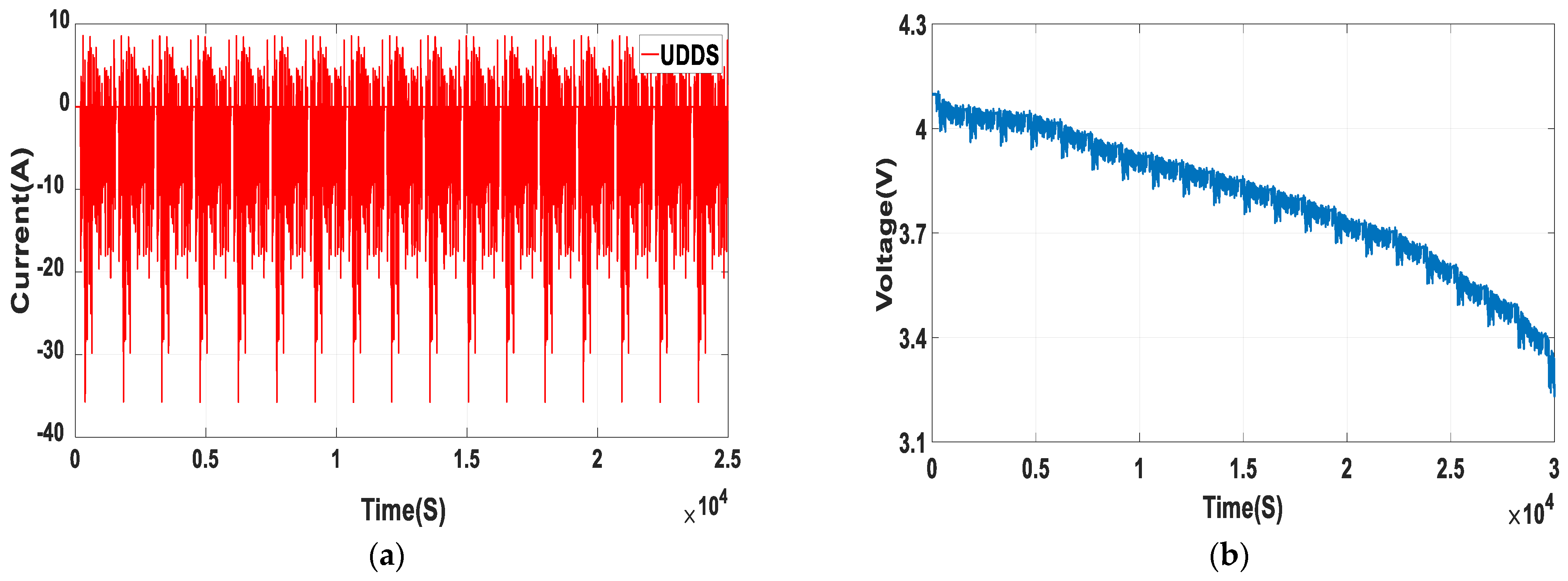
The current and voltage tested under the UDDS working conditions are shown in Figure 11a,b. As can be seen, these working conditions are very complicated, allowing the robustness of the algorithm to be better tested. Figure 12a,b illustrate the estimation effects of the three algorithms under these working conditions. The results indicate that the robustness and estimation accuracy of the FOUHIF algorithm are the best, with RSME, MAE, and ME reduced to 0.97, 0.74, and 1.61%, respectively. The maximum error in the SOC estimated by this algorithm occurred at the 22,463th second. Figure 12c,d illustrate the terminal voltage values and their errors predicted by the three algorithms. As revealed from the experiments, the FOUHIF algorithm had the best evaluation effect, with a maximum absolute error in the estimated terminal voltage of just 4.94 mV.

Table 5. Statistical data of terminal voltages under UDDS cycles.

	RSME (10%)	MAE (10%)	ME (10%)
FOUHIF	0.97	0.73	1.61
FOUKF	1.73	0.96	1.94
UKF	1.94	1.23	2.22

shows the error of SOC estimation by three algorithms under UDDS condition.

Under the UDDS working conditions, the uncertainty analysis of the three estimation methods was conducted to select the time period when the battery was standing, ranging from 30,147 to 30,500 s. The uncertainty components of the UKF, FOUKF and FOUHIF estimation methods caused by repeated measurements were $1.3\times {10}^{-3}$, $7.9\times {10}^{-4}$, and $1.2\times {10}^{-4}$, respectively. The uncertainties caused by equipment indication errors were $7.2\times {10}^{-4}$, $4.8\times {10}^{-4}$, and $4.1\times {10}^{-4}$, respectively. The standard uncertainties of the three methods were $1.5\times {10}^{-3}$, $9.2\times {10}^{-3}$, and $1.6\times {10}^{-4}$. For the selected measurement time interval, the measurement results of the three measurement methods were $0.898\pm 0.0015$, $0.908\pm 0.00092$, and $0.904\pm 0.00016$, respectively. Therefore, in terms of uncertainty, the FOUHIF algorithm had the highest reliability when analyzing the three measurement methods.

6. Conclusions

In this paper, by using the fractional order battery model as the core component, an analysis was made on the advantages of several models from the perspectives of electrochemistry and mathematical modeling. The results revealed that the internal chemical reaction process of lithium batteries depicted by the fractional order model is more comprehensive. On this basis, the FOUHIF algorithm was proposed as a method for estimating the SOC. In this algorithm, estimation accuracy and speed could be improved by using UT, and colored noise could be filtered out using a cost function. Furthermore, the parameters of the second order RC model and the fractional order model were separately identified, and the terminal voltage estimation effects of the two types of models were tested under HPPC working conditions. The experimental results show that the terminal voltage estimated by the fractional order model was more accurate, with absolute error kept within 5 mV. Following this, the estimation effect of the FOUHIF algorithm was verified under NEDC and UDDS working conditions. At the same time, with the error of the initial value of the SOC artificially set as 30% and 50%, the estimation result of this algorithm was improved significantly, compared with those of the FOUKF and UKF algorithms under the same experimental conditions. Under the two working conditions, the maximum absolute error in the estimated value of the SOC was reduced to 1.86% and 1.61%, with the error of the estimated terminal voltage kept within the range of 0–5.29 mV. The experimental results revealed that the FOUHIF algorithm had high robustness and estimation accuracy.