Adaptive Neuro-Fuzzy Inference System-Based Maximum Power Tracking Controller for Variable Speed WECS

Abstract

This paper proposes an adaptive neuro-fuzzy inference system (ANFIS) maximum power point tracking (MPPT) controller for grid-connected doubly fed induction generator (DFIG)-based wind energy conversion systems (WECS). It aims at extracting maximum power from the wind by tracking the maximum power peak regardless of wind speed. The proposed MPPT controller implements an ANFIS approach with a backpropagation algorithm. The rotor speed acts as an input to the controller and torque reference as the controller’s output, which further inputs the rotor side converter’s speed control loop to control the rotor’s actual speed by adjusting the duty ratio for the rotor side converter. The grid partition method generates input membership functions by uniformly partitioning the input variable ranges and creating a single-output Sugeno fuzzy system. The neural network trained the fuzzy input membership according to the inputs and alter the initial membership functions. The simulation results have been validated on a 2 MW wind turbine using the MATLAB/Simulink environment. The controller’s performance is tested under various wind speed circumstances and compared with the performance of a conventional proportional–integral MPPT controller. The simulation study shows that WECS can operate at its optimum power for the proposed controller’s wide range of input wind speed.

1. Introduction

Electricity is an undeniable source for the development of any nation. Life cannot be imagined without electricity in any sector, whether residential, commercial, or industrial. The generation of electricity depends on fossil fuels such as oil, coal, and natural gases. About 70% of the world’s electricity generation is done by coal and other fossil fuels. With the increase in population, the requirement for electricity is also accelerating at an alarming rate, demanding the increased consumption of fossil fuels. As a result, fossil fuel supplies exhaust. All these issues can be eliminated promisingly by renewable energy sources. Wind energy, solar energy, biomass energy, geothermal energy, and tidal energy are some of the well-established and developed renewable energy sources [1,2].

As a clean and green energy source, wind energy is the most effective option for mitigating pollution and meeting energy requirements [3]. Wind energy generation depends on weather conditions, so the power generation from wind energy fluctuates and does not fulfil load demand instantaneously. For reliable operation and performance, an appropriate control strategy should be adopted. Therefore, the operation of the wind energy conversion system (WECS) in obtaining optimal power has become critical due to the intermittent behaviour of wind flow. To resolve this problem and to use WECS more economically and efficiently, MPPT technology needs to be implemented to extract optimal power at variable wind speed conditions.

In the literature, mainly two types of wind energy generation (WEG), variable speed WEG [4], and fixed-speed WEG [5], are available. The variable speed WEG is more advantageous than fixed-speed WEG; it offers wide wind speed range operation, better power-capturing capability, and improved overall efficiency. The doubly fed induction generator (DFIG) is most dominant for variable speed operation applications. It uses reduced capacity power converters, about one-fourth of the system-rated capacity, and is less expensive and easier to maintain [6,7]. The DFIG also provides good damping for the weak grids. The operation and control of wind turbines have been improved today, and the credit goes to the developments in the power electronics industry.

The drawbacks of both the permanent magnet synchronous generator (PMSG) [8] and squirrel cage induction generator (SCIG) [9] WECS are that they need a power converter rated at the total system power rating, which increases their cost. Filters for inverter outputs and EMI are rated for the rated output power, complicating and increasing filter design costs. Additionally, converter efficiency has a significant impact on overall system efficiency throughout the entire operating range.

Most of the WECS are equipped with DFIG using back-to-back power electronic converters in the wind industry [10,11]. Because the converter does not have to transmit the total power generated by the DFIG, its power rating is smaller than the overall machine rating. Such WECS has decreased the cost of inverters because generally, the inverter rating is one fourth of total system power. Additionally, it decreased the cost of inverter and EMI filters since filters are rated for one fourth of total system power, and inverter harmonics represent a smaller proportion of total system harmonics. The higher cost of the wound rotor induction machine than the SCIG is compensated by the smaller size of the power converters and increased energy production [12]. The maximum power point tracking control is implemented utilizing a machine-side control mechanism in such a system.

Maximum power point control (MPPT) algorithms are among the best techniques to extract the maximum possible power at various wind speeds in wind turbine systems. The MPPT algorithms protect the system from overload and various lightening surges [13,14]. Additionally, MPPT assists in stabilizing the output voltage in the presence of higher and lower wind speeds than the rated wind speed.

In the literature [15,16,17], various MPPT algorithms have extensively been discussed. The hill-climbing search (HCS), optimum relation-based MPPT (ORB), and the incremental conductance (INC) are all classified as direct power control (DPC)-based MPPT algorithms. While optimal torque control (OTC), power signal feedback (PSF), and tip-speed ratio (TSR) algorithms are included in the category of indirect power control (IPC)-based MPPT algorithms. In addition, fuzzy-logic and neural network-based control has been developed [18].

HCS, also known as perturbation and observation, is a resilient, unreliable technique based on previous WT characteristics knowledge. This algorithm provides the local maximal point for the given function [19]. The likelihood of identifying the wrong direction to achieve the most significant power point under a sudden change in wind direction is a disadvantage of this method. Using a modified version of the HCS method, [20,21] was able to address the issue of incorrect direction movement under changing wind speeds.

The ideal relationship between quantities such as WT power output, converter DC voltage, power, current, and speed is required by the ORB-based MPPT algorithm [22,23]. Fast-tracking and no need for sensors are the main advantages of this technique. However, a thorough understanding of the characteristic curves of turbine power and DC current at different wind speeds is required. By observing the optimum current curve, the MPP can be tracked [24].

The INC algorithms are completely independent of sensor needs and the specification of wind turbine and generator parameters. Therefore, systems employed with this algorithm reduce the system’s cost and improve reliability [25]. According to the authors in [26,27], the operating point of the MPPT may be determined using the power-speed slope. The disadvantage of this method is that it becomes unstable when the inertia of the turbine varies under a variable speed wind scenario [28]. A new method called as the fractional order INC (FO-INC) is presented in [27] to address the instability issue at different wind speeds. For fast changes, variable step size is used in tracking the MPP under variable wind conditions.

The PSF-based MPPT approach makes use of a power control loop which incorporates information about WT’s maximum power curve [12]. While the TSR-based MPPT controller is easy to build and highly efficient, it has a high operating cost. The drawback of this method is it needed optimal power coefficient and optimal tip-speed ratio [29].

The OTC technique involves changing the generator torque based on the most significant power reference torque at any given wind speed [18]. The main advantages of this method are fast response, efficiency, and simplicity. Due to the absence of direct wind speed measurement, changes in wind speed are not reflected in the reference signal [16].

MPPT control techniques based on fuzzy logic offer the benefits of rapid convergence, parameter independence, and acceptance of noisy and incorrect data [30]. The articles [31,32] provide a data-driven design approach for generating a Takagi–Sugeno–Kang (TSK) fuzzy model for MPPT control. Although the fuzzy model offers many advantages over other techniques, the main drawback is that it cannot be used for every issue. Additionally, it necessitates an examination of the parameter used to assign linguistic variables.

The artificial neural network (ANN) is another method to determine the maximum power peak by taking various input variables and processing them to obtain the maximum power [33]. Each neural network (NN) contains an input layer, a hidden layer, and an output layer. There is really no constraint on the number of nodes assigned, and they may vary as per the demand. The ANN-based controller is a more efficient and reliable alternative than conventional controllers for extracting the maximum amount of power from wind’s available kinetic energy. The disadvantages of NN include their black box structure, increased computing load, overfitting issue, and empirical nature of model development. This technique necessitates the use of a look-up table containing predefined data [34].

The membership function type, number of rules, and correct selection of parameters of FLC are essential to obtain desired performance in the system. Selecting suitable fuzzy rules, membership functions, and their definitions in the universe of discourse invariable involves painstaking trial-error [35]. The adaptive neuro-fuzzy inference system (ANFIS) is a scheme derived from a synthesis between the neural network and fuzzy inference system [36]. Similar to the method of training a neural network, the membership function parameters have been fine-tuned using adaptive neuro-learning methods. A neural network enhances the adaptability of the model. The primary purpose of using the ANFIS approach is to realize the fuzzy system by using neural network methods automatically. The ANFIS combines the capability of fuzzy reasoning in handling the uncertainties and the capability of ANN in learning from processes [36].

In this paper, an ANFIS MPPT controller is used for maximum power tracking. The generator rotor speed is input to the MPPT controller training input value, and the optimum torque reference is selected as the target value.

The following is the structure of the paper. Section 1 discusses renewable energy importance and the literature of MPPT algorithms employed in wind energy conversion systems. The modeling of doubly fed induction generator-based WECS is given in Section 2. Section 3 deals with rotor side control with maximum power point tracking control. Section 4 defines the ANFIS MPPT controller for achieving maximum power point along with the training process. Section 5 illustrates the performance of the ANFIS approach. A comparison with another conventional approach is also carried out in this section. Finally, Section 6 summarizes the conclusion.

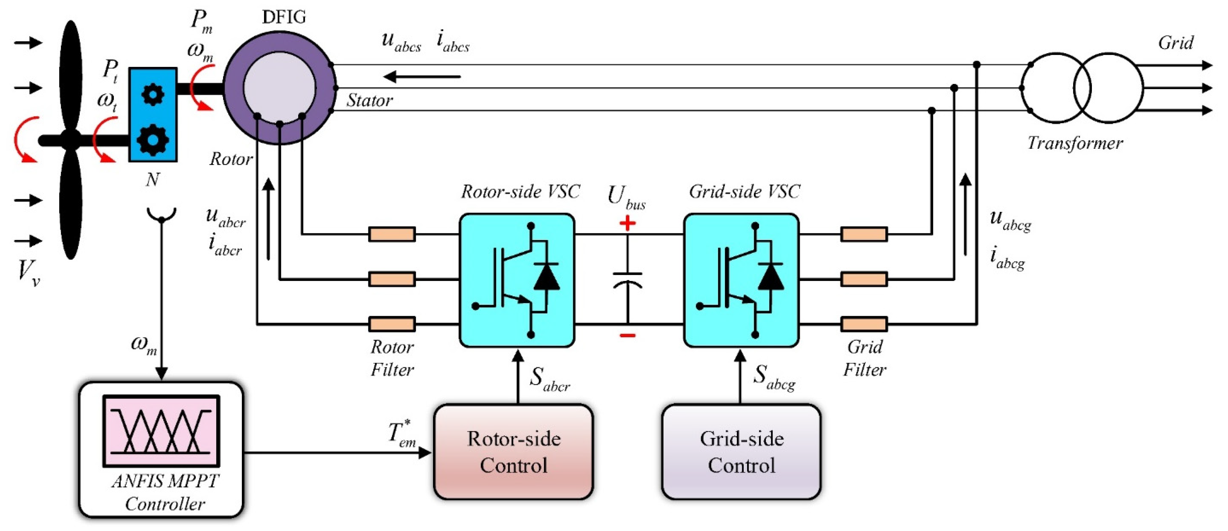
2. Modeling of Doubly Fed Induction Generator-Based WECS

Configuration of the grid-connected DFIG-based WECS considered in this study is shown in Figure 1, which consists of a turbine system connected to the DFIG generator through a gear system. The stator winding of the DFIG is directly connected to the grid. In contrast, the rotor of the DFIG is connected to the grid via a back-to-back power converter. In addition, a MPPT controller is connected to the RSC control of the WECS.

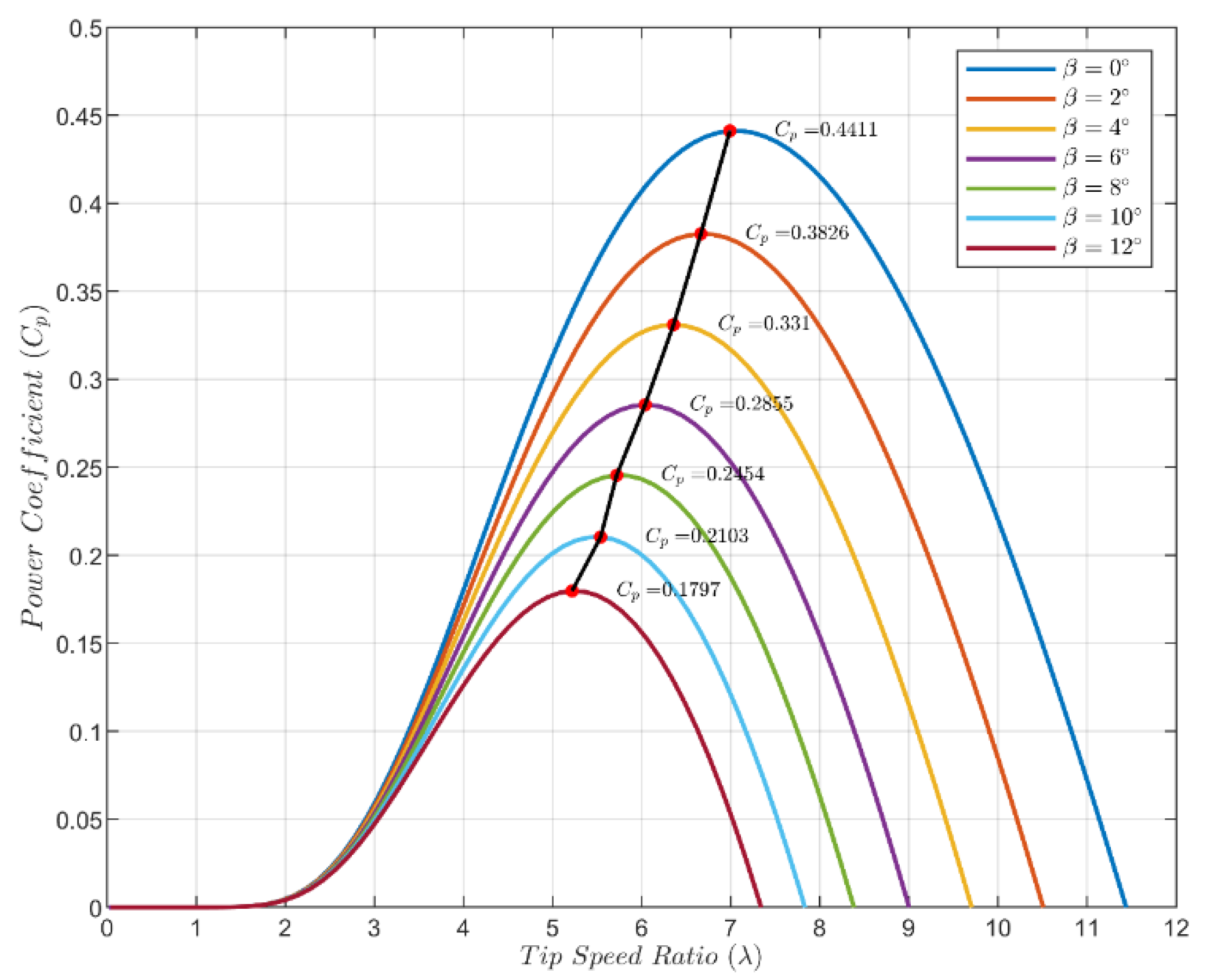
2.1. Wind Turbine Modeling

The equation for the amount of power derived by the wind turbine from the wind is expressed in (1) [37]:

$$P_t=\frac{1}{2}\rho \pi R^2{V}_v^3{C}_p\left(\lambda ,\beta \right)$$

(1)

where ρ is the air density measured in kilograms per cubic meter (kg/m³), R is the rotor radius of the turbine measured in meter (m), $V_v$ presents the wind speed measured in meter per second (m/s), $C_p\left(\lambda ,\beta \right)$ presents the power coefficient expressed as a function of the tip-speed ratio (λ) and the pitch angle (β).

λ is expressed in (2):

$$\lambda =\frac{R{\omega }_t}{V_v}$$

(2)

where ${\omega }_t$ is the angular rotational speed of the wind turbine rotor (rad/sec).

$C_p\left(\lambda ,\beta \right)$ is expressed by (3) [37]:

$$C_p\left(\lambda ,\beta \right)=c_1\left(\frac{c_2}{{\lambda }_i}-c_3\beta -c_4{\beta }^{c_5}-c_6\right).e^{\frac{-c_7}{{\lambda }_i}}.$$

(3)

${\lambda }_i$ is given in (4):

$${\lambda }_i=\frac{1}{\lambda +0.02\beta }-\frac{0.003}{{\beta }^3+1}$$

(4)

where $c_1=0.73;c_2=151;c_3=0.58;c_4=0.002;c_5=2.4;c_6=13.2;c_7=18.4$ The turbine generated torque is expressed in (5) [37]:

$$T_t=\frac{P_t}{{\omega }_t}$$

(5)

2.2. DFIG Modeling

The following equations describe the DFIG model. The voltage vectors of the stator and rotor are expressed in (6) and (7), respectively [36]:

$${\overrightarrow{u}}_s=R_s{\overrightarrow{𝑖}}_s+\frac{d{\overrightarrow{\psi }}_s}{dt}+j{\omega }_s{\overrightarrow{\psi }}_s\Rightarrow \{\begin{array}{c}{u}_{ds}=R_s{𝑖}_{ds}+\frac{d{\psi }_{ds}}{dt}-{\omega }_s{\psi }_{qs}\\ u_{qs}=R_s{𝑖}_{qs}+\frac{d{\psi }_{qs}}{dt}+{\omega }_s{\psi }_{ds}\end{array}$$

(6)

$${\overrightarrow{u}}_r=R_s{\overrightarrow{𝑖}}_r+\frac{d{\overrightarrow{\psi }}_r}{dt}+j{\omega }_r{\overrightarrow{\psi }}_r\Rightarrow \{\begin{array}{c}{u}_{dr}=R_r{𝑖}_{dr}+\frac{d{\psi }_{dr}}{dt}-{\omega }_r{\psi }_{qr}\\ u_{qr}=R_r{𝑖}_{qr}+\frac{d{\psi }_{qr}}{dt}+{\omega }_r{\psi }_{dr}\end{array}$$

(7)

where $u_{ds}$, $u_{qs}$, $u_{dr}$, and $u_{qr}$: Voltages at the stator and rotor in the d–q frame, respectively. $i_{ds}$, $i_{qs}$, $i_{dr}$, and $i_{qr}$: Currents in the stator and rotor in the d–q frame, respectively. $R_r$, $R_s$, ${\omega }_s$, and ${\omega }_r$: Stator and rotor phase resistances and angular velocity, respectively.

The flux vectors for the stator and rotor are denoted in (8) and (9), respectively [37]:

$${\overrightarrow{\psi }}_s=L_s{\overrightarrow{𝑖}}_s+L_m{\overrightarrow{𝑖}}_r\Rightarrow \{\begin{array}{c}{\psi }_{ds}=L_s{𝑖}_{ds}+L_m{𝑖}_{dr}\\ {\psi }_{qs}=L_s{𝑖}_{qs}+L_m{𝑖}_{qr}\end{array}$$

(8)

$${\overrightarrow{\psi }}_r=L_m{\overrightarrow{𝑖}}_s+L_r{\overrightarrow{𝑖}}_r\Rightarrow \{\begin{array}{c}{\psi }_{dr}=L_m{𝑖}_{ds}+L_r{𝑖}_{dr}\\ {\psi }_{qr}=L_m{𝑖}_{qs}+L_r{𝑖}_{qr}\end{array}$$

(9)

where ${\overrightarrow{\psi }}_s$, ${\overrightarrow{\psi }}_r$ are the flux vectors for stator and rotor, respectively. ${\psi }_{ds}$, ${\psi }_{qs}$ are the fluxes along the d–q axis stator. ${\psi }_{dr}$, ${\psi }_{qr}$ are the fluxes along with the d–q axis rotor. $L_s$, $L_r$: Leakage inductances in the stator and rotor phases, $L_m$: Mutual inductance between stator and rotor, p: is the generator pole pair count.

The expression of electromagnetic torque is expressed in (10) [37]:

$$T_{em}=\frac{3}{2}p\frac{L_m}{L_s}\left({\psi }_{qs}{i}_{dr}-{\psi }_{ds}{i}_{qr}\right)$$

(10)

The active and reactive power equations of the stator and rotor are expressed in (11) and (12) [37]:

$$\{\begin{array}{c}{P}_s=\frac{3}{2}\left(u_{ds}{i}_{ds}+u_{qs}{i}_{qs}\right)\\ Q_s=\frac{3}{2}\left(u_{qs}{i}_{ds}-u_{ds}{i}_{qs}\right)\end{array}$$

(11)

$$\{\begin{array}{c}{P}_r=\frac{3}{2}\left(u_{dr}{i}_{dr}+u_{qr}{i}_{qr}\right)\\ Q_r=\frac{3}{2}\left(u_{qr}{i}_{dr}-u_{dr}{i}_{qr}\right)\end{array}$$

(12)

where $P_s$, $Q_s$ presents stator active and reactive power. $P_r$, $Q_r$ presents rotor active and reactive power. $T_{em}$ is the electromagnetic torque.

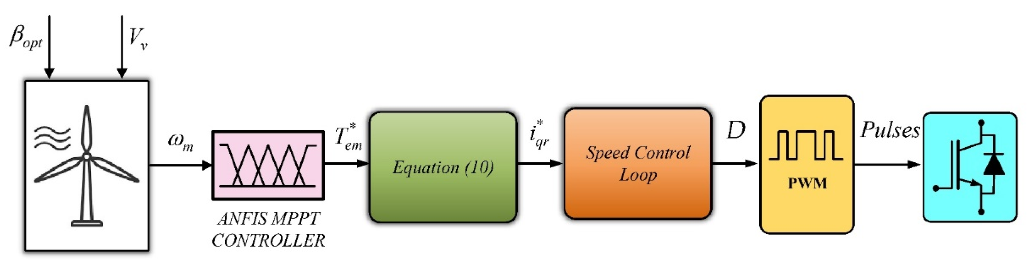
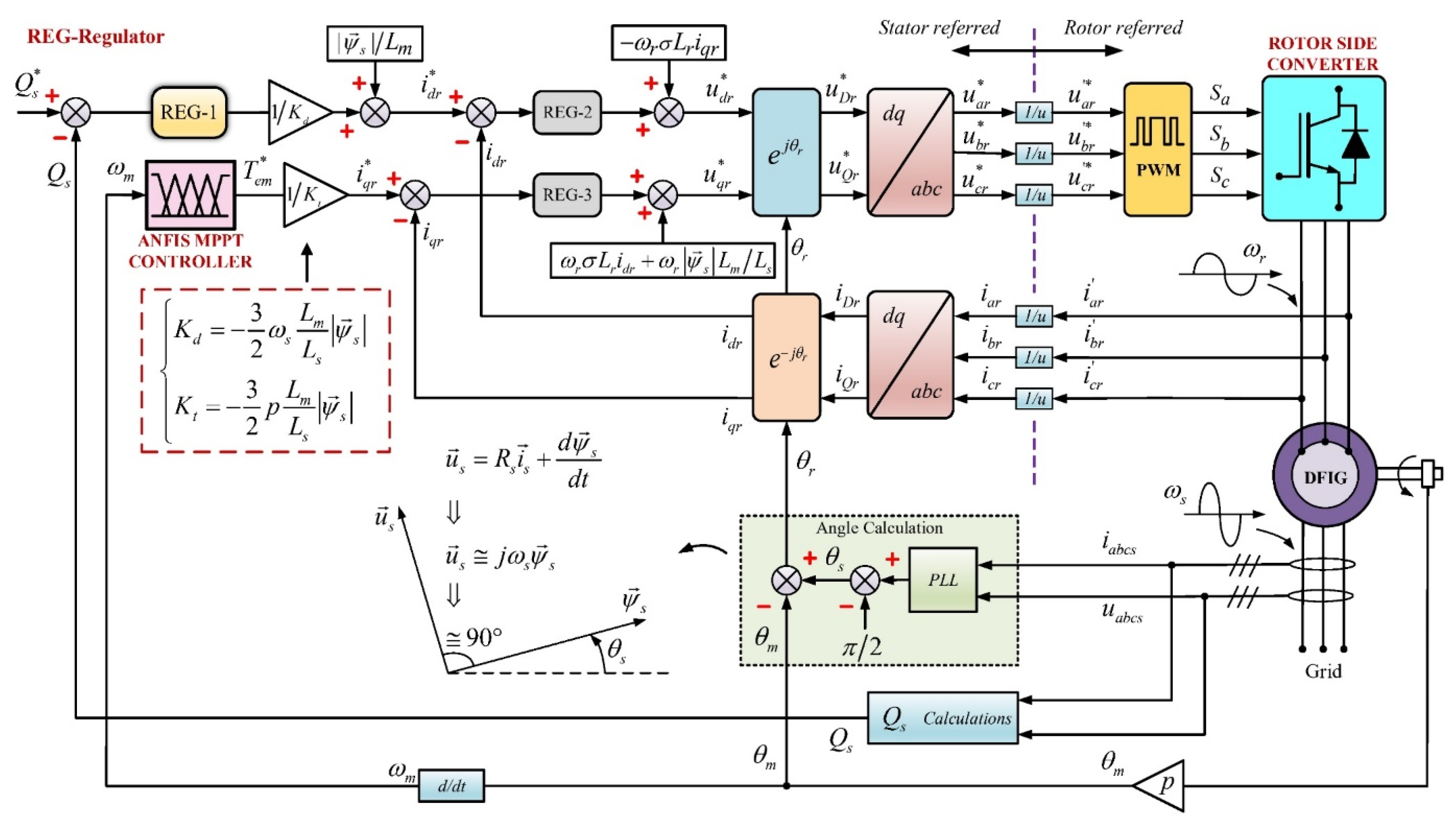
3. Rotor Side Control with Maximum Power Point Tracking

The RSC is responsible for the voltage applied to the rotor winding of the DFIG. To derive the voltage equation in dq reference frame, from the DFIG model in the previous section, replacing Equations (8) and (9) in Equation (7) and considering ${\psi }_{qs}=0$ we get the following equation as a function of the rotor currents and stator flux [37]:

$$\{\begin{array}{c}{u}_{dr}=R_r{i}_{dr}+\sigma L_r\frac{d{i}_{dr}}{dt}-{\omega }_r\sigma L_r{i}_{qr}+\frac{L_m}{L_s}\frac{d|{\overrightarrow{\psi }}_s|}{dt}\\ u_{qr}=R_r{i}_{qr}+\sigma L_r\frac{d{i}_{qr}}{dt}+{\omega }_r\sigma L_r{i}_{dr}+{\omega }_r\frac{L_m}{L_s}\frac{d|{\overrightarrow{\psi }}_s|}{dt}\end{array}$$

(13)

where $\sigma =1-\frac{L_m^2}{L_s{L}_r}$. Assuming negligible voltage drop in the stator winding resistance and stator flux are constant because of the constant grid quantities, consequently, zero. It can be seen from Equation (13) that dq component of rotor current can be controlled using regulators. The reactive power proportional–integral (PI) regulator represented as REG-1. The equal PI regulator for both d and q current loop are chosen as REG-2 and REG-3, respectively. Actual values are considered for tunning of the gain parameters of the regulators. The gain parameters for all three regulators are presented in

Table 1. The gain parameters of PI regulators in rotor side control.

Gains	REG-1	REG-2	REG-3
Proportional	10,160	0.5771	0.5771
Integral	406,400	491.5995	491.5995

. The control must be performed on the dq components, so rotor voltage and current are transformed into dq components using abc–dq transform. Θ_s is obtained by first estimate the stator voltage vector and subtracting angle π/2. The phase-locked loop (PLL) is used for grid synchronization, which also supports in rejection of minor disturbances. The “u” defines the stator-rotor turn ratio that is 1/3. Figure 2 illustrates the complete vector control of the DFIM with MPPT controller.

The torque expressions in dq frame can be given by:

$$T_{em}=\frac{3}{2}p\frac{L_m}{L_s}\left({\psi }_{qs}{i}_{dr}-{\psi }_{ds}{i}_{qr}\right)\Rightarrow T_{em}=-\frac{3}{2}p\frac{L_m}{L_s}{\psi }_{ds}{i}_{qr}\Rightarrow T_{em}=K_t{i}_{qr}$$

(14)

The stator reactive power expressions in dq frame can be given by:

$$Q_s=\frac{3}{2}\left(u_{qs}{i}_{ds}-u_{ds}{i}_{qs}\right)=-\frac{3}{2}{\omega }_s\frac{L_m}{L_s}|{\overrightarrow{\psi }}_s|\left(i_{dr}-\frac{|{\overrightarrow{\psi }}_s|}{L_m}\right)\Rightarrow Q_s=K_q\left(i_{dr}-\frac{|{\overrightarrow{\psi }}_s|}{L_m}\right)$$

(15)

Equation (14) reveals that the i_qr is proportional to the T_em to control torque with i_qr. Expression in Equation (15) reveals that d component of rotor current i_dr controls the Q_s. Therefore, because of the orientation chosen, it can be seen that both rotor current components independently allow us to control the torque and reactive stator power.

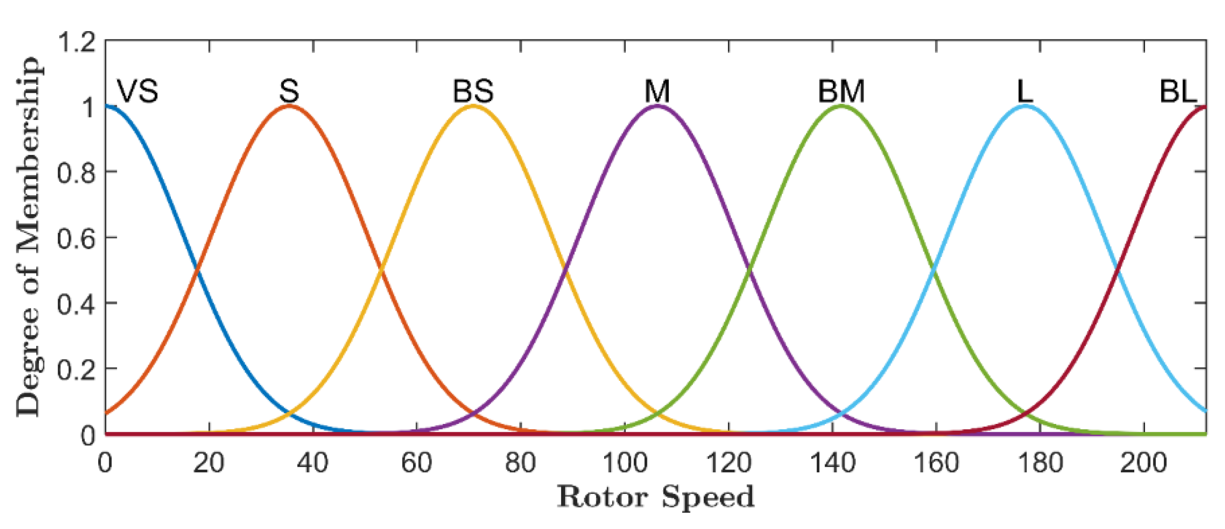
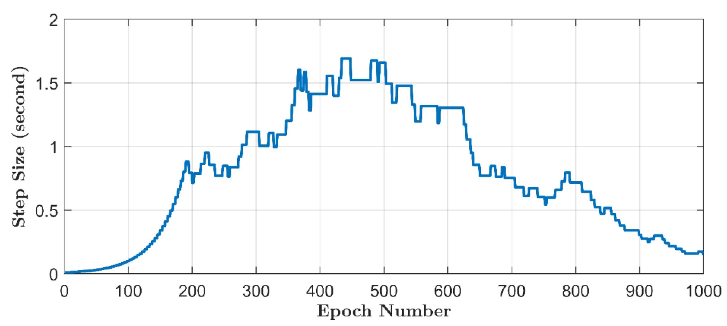
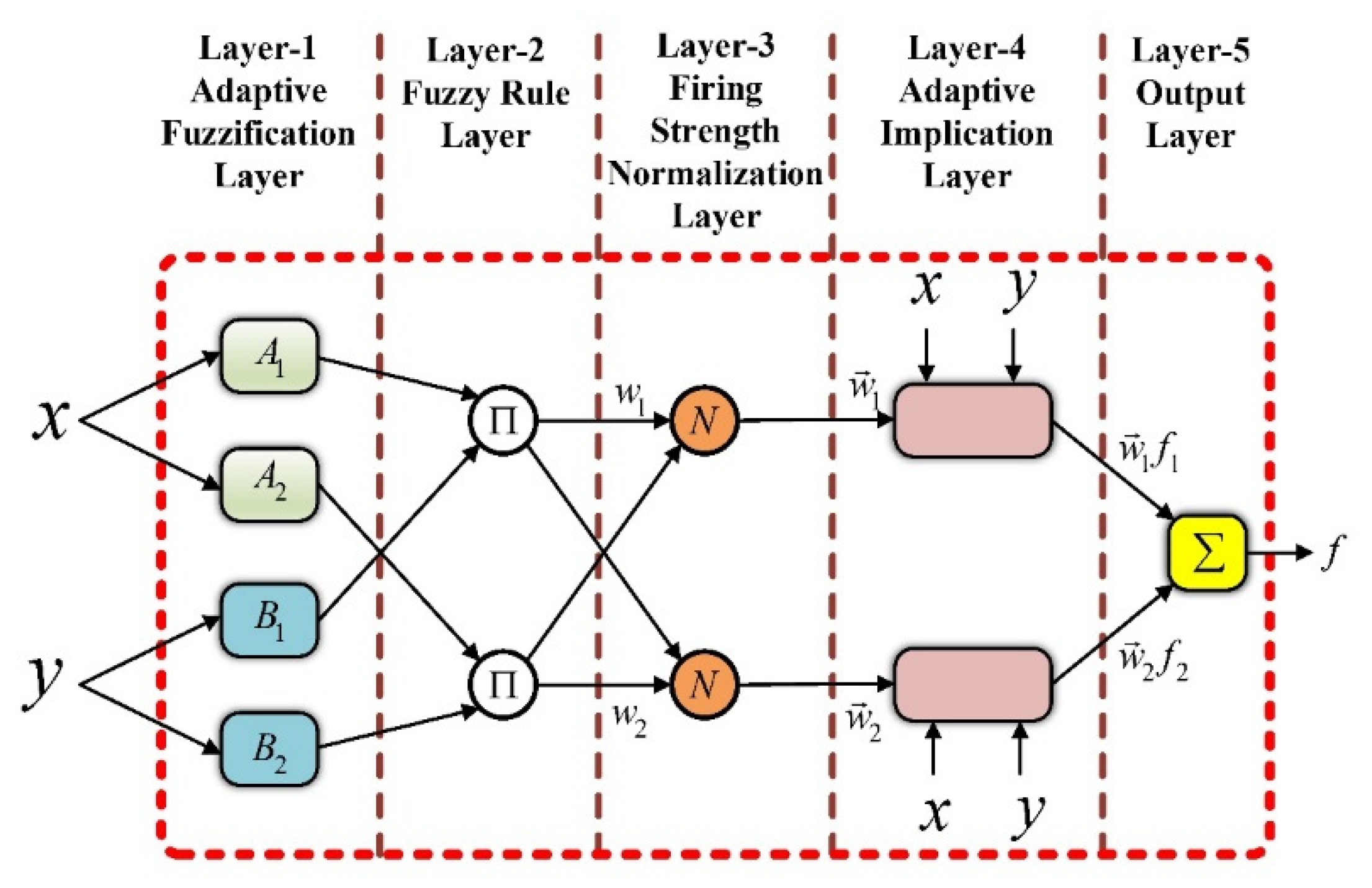
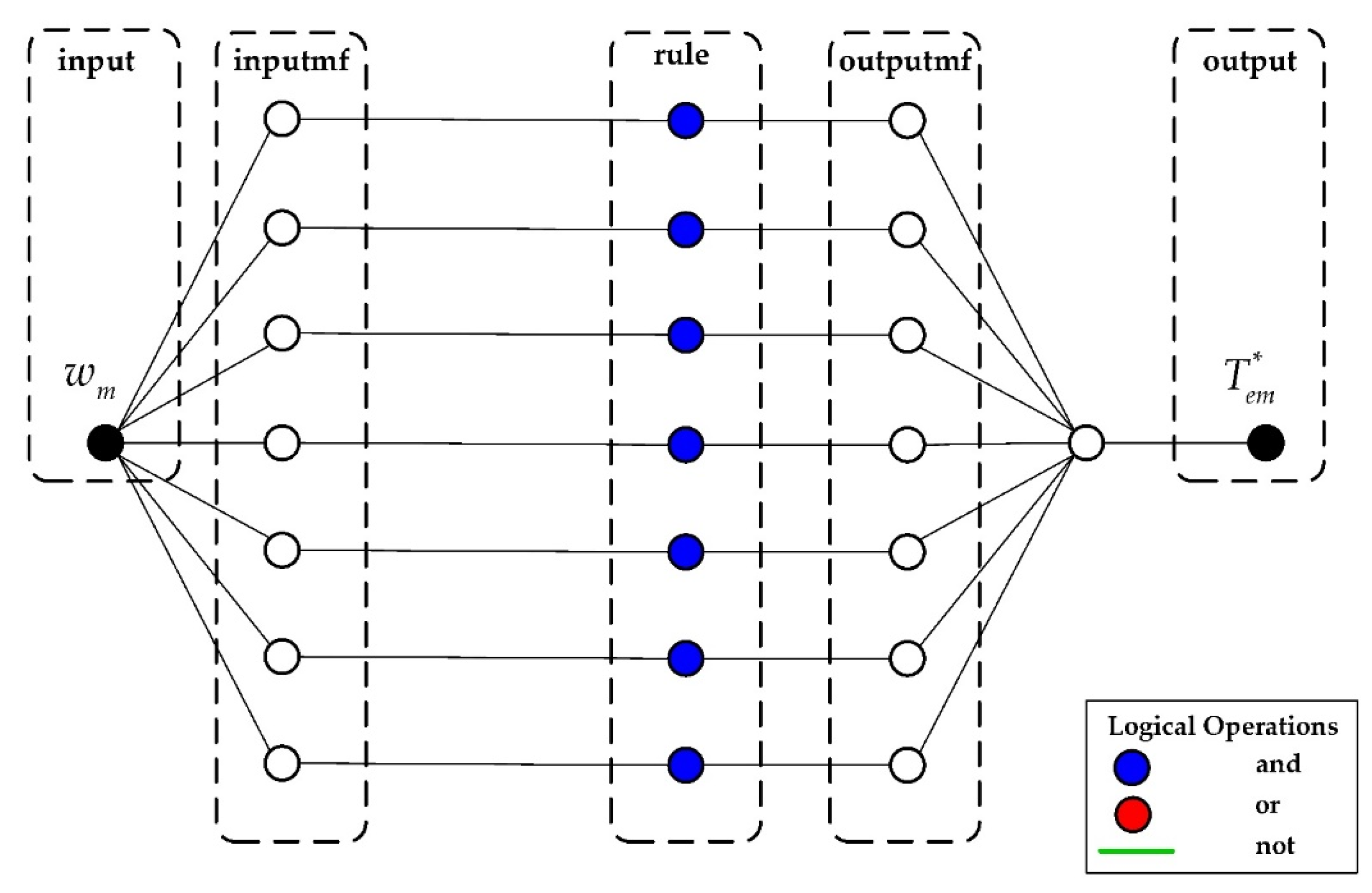
4. ANFIS Maximum Power Point Tracking Control

The adaptive neuro-fuzzy inference method is a highly effective technique that incorporates both fuzzy control and artificial neural network concepts [31,38,39]. Due to the combined influence of fuzzy and neural networks, it is an excellent learner and interpreter [40]. The ANFIS controller determines which membership function to use. The general structure of ANFIS consists of five layers, as shown in Figure 3.

• Layer 1, the adaptive fuzzification layer is composed of user-specified input variables and membership functions (MF).
• Layer 2, the fuzzy rule layer checks the degree of MF, and the corresponding fuzzy set is selected and input to the next layer.
• Layer 3, the firing strength normalization layer evaluates weight for each normalized node.
• Layer 4, the adaptive implication layer outputs values in accordance with inference rules, and each neuron is normalized.
• Layer 5, the output layer adds all of the inputs from layer 4 and transforms the fuzzy values to a crisp value.

The developed ANFIS has single input as rotor speed. The instantaneous torque reference is determined as the output from the ANFIS network. In the developed MPPT controller, the ANFIS first-order Sugeno model as well as with fuzzy IF-THEN rules of Takagi and Sugeno type are used. A backpropagation algorithm trains the ANFIS-based MPPT controller.

Figure 4 illustrates the block diagram of the proposed ANFIS MPPT control. The generated optimal torque ($T_{em}^{*}$) is used to determine rotor quadrature current reference ($i_{qr}^{*}$) applied to the speed control loop of RSC control that controls the actual rotor speed by adjusting the duty ratio of the RSC. The control objective of the converter is to maximize the output power delivered to the grid.

Figure 5 depicts the architecture of the developed ANFIS controller in MATLAB/Simulink using Neuro-Fuzzy Designer. The ANFIS details are given in

Table 2. The ANFIS parameters information.

Parameter	Value	Parameter	Value
Number of nodes	32	Total number of parameters	28
Number of linear parameters	14	Number of training data pairs	10,000,001
Number of nonlinear parameters	14	Number of fuzzy rules	7

. The trial-and-error method is used for choosing the number and shape of MFs as there is no exact method for choosing the MFs in the literature. Seven Gaussian MFs were selected for this study because they had the lowest root-mean-square error (RMSE) of 0.098280. The primary reason why Gaussian MFs were chosen is that they have the fewest parameters (Only two parameters mean and standard deviation). To define the membership functions and fuzzy rules, the grid partition method is used, generating input membership functions by uniformly partitioning the input variable ranges and creating a single-output Sugeno fuzzy system. Each input membership function combination is represented by a single rule in the fuzzy rule base.

Speed is taken as an input to the ANFIS MPPT controller, and it outputs the torque reference. The controller is trained for 1000 epochs. The controller has one input with seven membership functions (MFs). The initial generated input speed membership functions for training are shown in Figure 6, which utilize seven rules. The details of the initial seven input membership functions derived from Equation (13) are presented in

Table 3. Initial input membership function details.

Membership Function Name	Type	Parameter
		Standard Deviation	Mean
Very Small (VS)	Gaussian	15.047	−3.3549 × 10−13
Small (S)	Gaussian	15.047	35.433
Big Small (BS)	Gaussian	15.047	70.865
Medium (M)	Gaussian	15.047	106.3
Big Medium (BM)	Gaussian	15.047	141.73
Large (L)	Gaussian	15.047	177.16
Big Large (BL)	Gaussian	15.047	212.6

.

The neural network tuned input speed membership functions is shown in Figure 7. The tunned membership functions details are presented in

Table 4. Neural network tunned input membership function details.

Membership Function Name	Type	Parameter
		Standard Deviation	Mean
Very Small (VS)	Gaussian	26.909	5.1594
Small (S)	Gaussian	30.952	33.765
Big Small (BS)	Gaussian	63.437	89.457
Medium (M)	Gaussian	34.224	107.28
Big Medium (BM)	Gaussian	33.967	138.56
Large (L)	Gaussian	35.116	183.63
Big Large (BL)	Gaussian	41.65	199.36

. As the output function in the Sugeno fuzzy inference system is selected as a linear function of the input, details of all seven output membership functions are given in

Table 5. Output membership function details.

Membership Function Name	Type	Parameter
		Lower Limit	Upped Limit
Very Small (VS)	Linear	1.9856	1145.1
Small (S)	Linear	7.3276	1244.4
Big Small (BS)	Linear	−4.8424	−5088.7
Medium (M)	Linear	−124.22	9248
Big Medium (BM)	Linear	−143.49	15,022
Large (L)	Linear	−98.038	7647.7
Big Large (BL)	Linear	−149.91	17,393

. Figure 8 shows the step size increase/decrease during the training. The root-mean-square error is shown in Figure 9. The expression for the Gaussian membership function is given in Equation (13):

$$f\left(x,\sigma ,c\right)=e^{\frac{-{\left(x-c\right)}^2}{2{\sigma }^2}}$$

(16)

where σ is the standard deviation, c is mean, and x is input value.

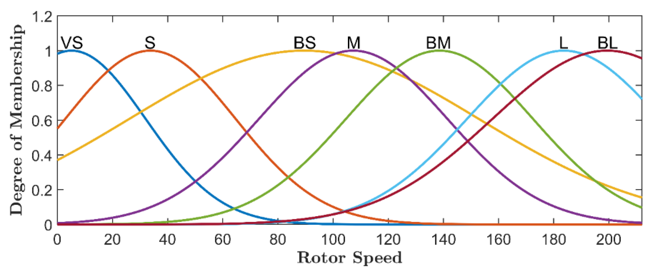
• The first layer consists of an input node as the variable. This layer is responsible for transform in input value to the next layer. Here, seven gaussian MFs with minimum = 0 and maximum = 1 are utilized, and corresponding node equations are given (17):

  $$O_i^1=\mu A_i\left(e_i\right)$$

  (17)

  where i = 1, 2, … 7, $O_i$ is the output of ith node in layer one, $A_i$ is the linguistic label, $e_i$ is the input to the node.

• The second layer verifies the weights of individual MFs. It accepts the first layer’s input values and serves as the MF for the corresponding input variables fuzzy sets. The second layer has non-adaptive nodes that multiply incoming signals and output the result as in (18):

  $$w_j=\mu A_i\left(e_1\right)\times \mu B_i\left(e_2\right)$$

  (18)

  where i = 1, 2, … 7 and j = 1, 2, … 7. The output from each node represents the firing strength of a rule.

• Each node in the third layer computes the activation level of each fuzzy rule, with the number of layers equal to the number of fuzzy rules. Each node of these layers generates the normalized weights. Each node calculates the ratio of the rule’s firing strength to the total of all rules’ firing strengths, that is, the normalized firing strength given in (19):

  $$w_j^{*}=\frac{w_j}{w_1+w_2\dots w_7}$$

  (19)

  where j = 1, 2, … 7.

• The fourth layer contains the output values obtained through rule inference. Node function of the fourth layer is given in (20):

  $$O_j^4=w_j^{*}{f}_j=w_j^{*}\left(p_j{e}_1+q_j{e}_2+r_j\right)$$

  (20)

The rule base is given as:

• If $e_1$ is $A_1$ and $e_2$ is $B_1$ then $f_1=p_1{e}_1+q_1{e}_2+r_1$;

• If $e_1$ is $A_2$ and $e_2$ is $B_2$ then $f_2=p_1{e}_1+q_2{e}_2+r_2$;

• If $e_1$ is $A_7$ and $e_2$ is $B_1$ then $f_7=p_7{e}_1+q_7{e}_2+r_7$,

where ($p_j$, $q_j$, $r_j$) is the parameter set and in this layer is referred to as consequent parameters, $O_j^4$ = output of the ith node in layer-4, $A_i$, $B_i$ = fuzzy membership function, i = 1,2, … 7 and j = 1, 2, … 7.

• The fifth layer is the output layer; it aggregates all of the fourth layer’s inputs and converts the fuzzy classification results into a crisp representation. This layer has a non-adaptive nature, having a single node with the output given in (21):

  $$y={\displaystyle \sum }_{j=1}^7{w}_j^{*}{f}_j={\displaystyle \sum }_{j=1}^7\left(\left(w_j^{*}{e}_1\right)p_j+\left(w_j^{*}{e}_2\right)q_j+\left(w_j^{*}\right)r_j\right)$$

  (21)

In practice, the proposed controller can be implemented using the Simulink HDL Coder toolbox that can generate code for the DSP’s and FPGA’s family chips of different vendors. The complete list of supported chips in the HDL coder and more details on this can be seen from the MathWorks official website [41].

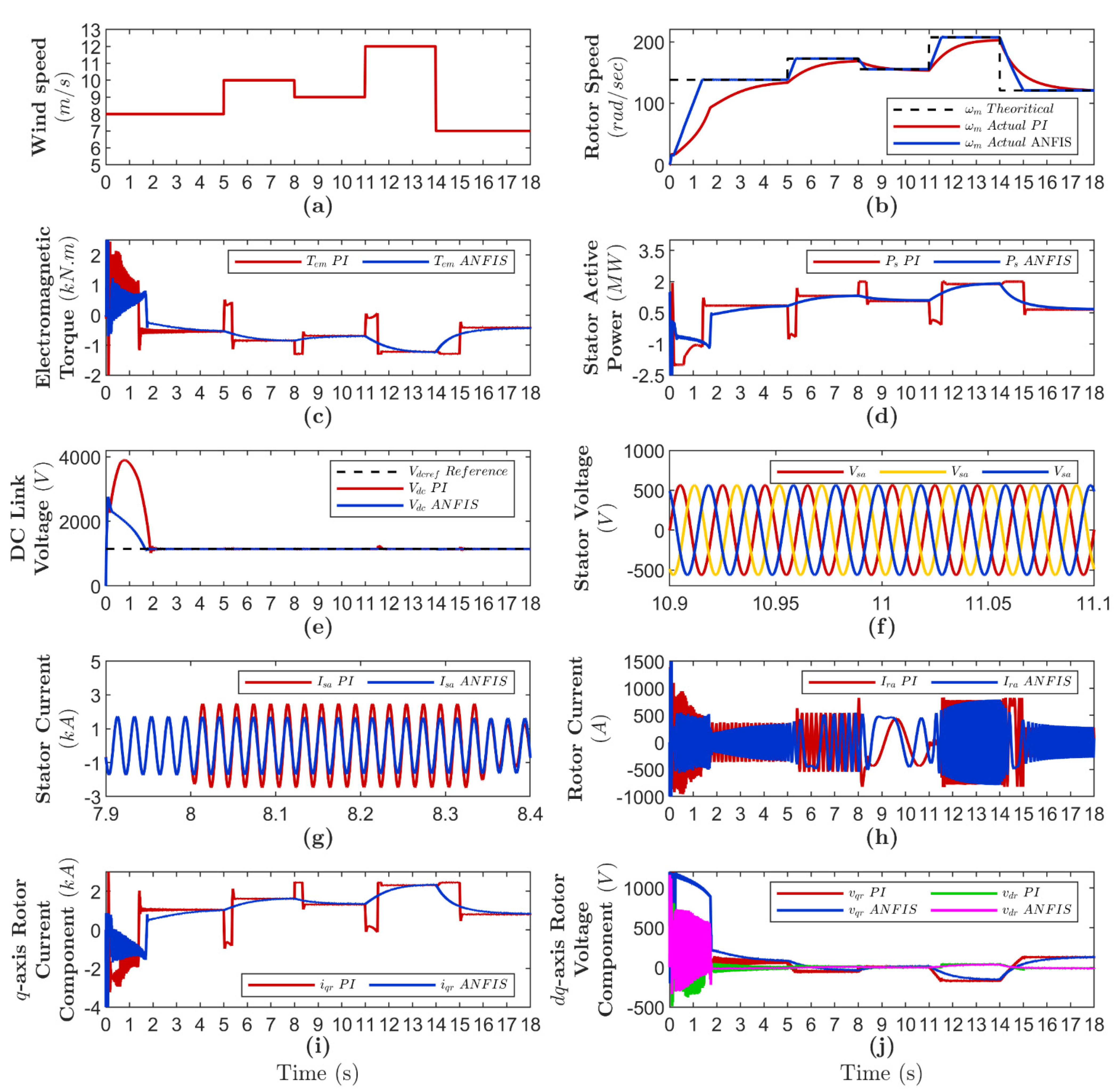
5. Simulation Result and Discussion

The effectiveness of the ANFIS MPPT controller for DFIG-based WECS under variable wind speed operation has been verified in MATLAB/Simulink environment. The simulation comparison results of the proportional–integral (PI) controller and the proposed ANFIS MPPT controller are present in the following figures.

In this work, β is set to zero and designed for the rated wind speed of 11 m/s. The simulated power characteristics at different wind speeds are presented in Figure 10.

$C_p-{\lambda }_i$ characteristics at different value of β is presented in Figure 9. The design presents that the maximum value $C_{pmax}$ is 0.4411 and the corresponding λ is 7, as shown in Figure 11. This value $C_{pmax}$ and λ is the optimum value for capturing peak power from the available wind power. Parameters of the WT are presented in

Table 6. WECS parameters.

Parameter	Value	Parameter	Value
Nominal wind speed	11 m/s	Frequency	50 Hz
Air density	1.225 kg/m3	Rated torque	12,732 N·m
Tip-speed ratio	7	Pole pair	2
Pitch angle	0°	Inertia	127 kg·m2
Power coefficient	0.4411	Gear ratio	100
Nominal power	2 MW	Radius of turbine	42 m

.

Three case studies are considered to analyze the performance of the proposed controller. Different input wind speed profiles are considered for all three cases.

Table 7. Input wind speed in all cases.

Time Duration (s)	Input Wind Speed (m/s)
	Case-I	Case-II	Case-III
0–5	6	12	8
5–8	7	11	10
8–11	8	10	9
11–14	9	9	12
14–17	10	8	7
17–20	11	7	7
20–23	12	6	7

shows an overview of all three cases of wind speed during the simulation study.

Simulation time responses of rotor speed (${\omega }_m$), electromagnetic torque ($T_{em}$), stator active power ($P_s$), DC-link voltage ($V_{dc}$), stator voltage ($V_s$), stator current of a-phase ($I_{sa}$), rotor current of a-phase ($I_{ra}$), q-axis rotor current component ($i_{qr}$), and d and q axis rotor voltage component ($v_{dr},v_{qr}$) with the change in system input wind speed ($V_v$) for PI controller and ANFIS controller are presented in following figures below.

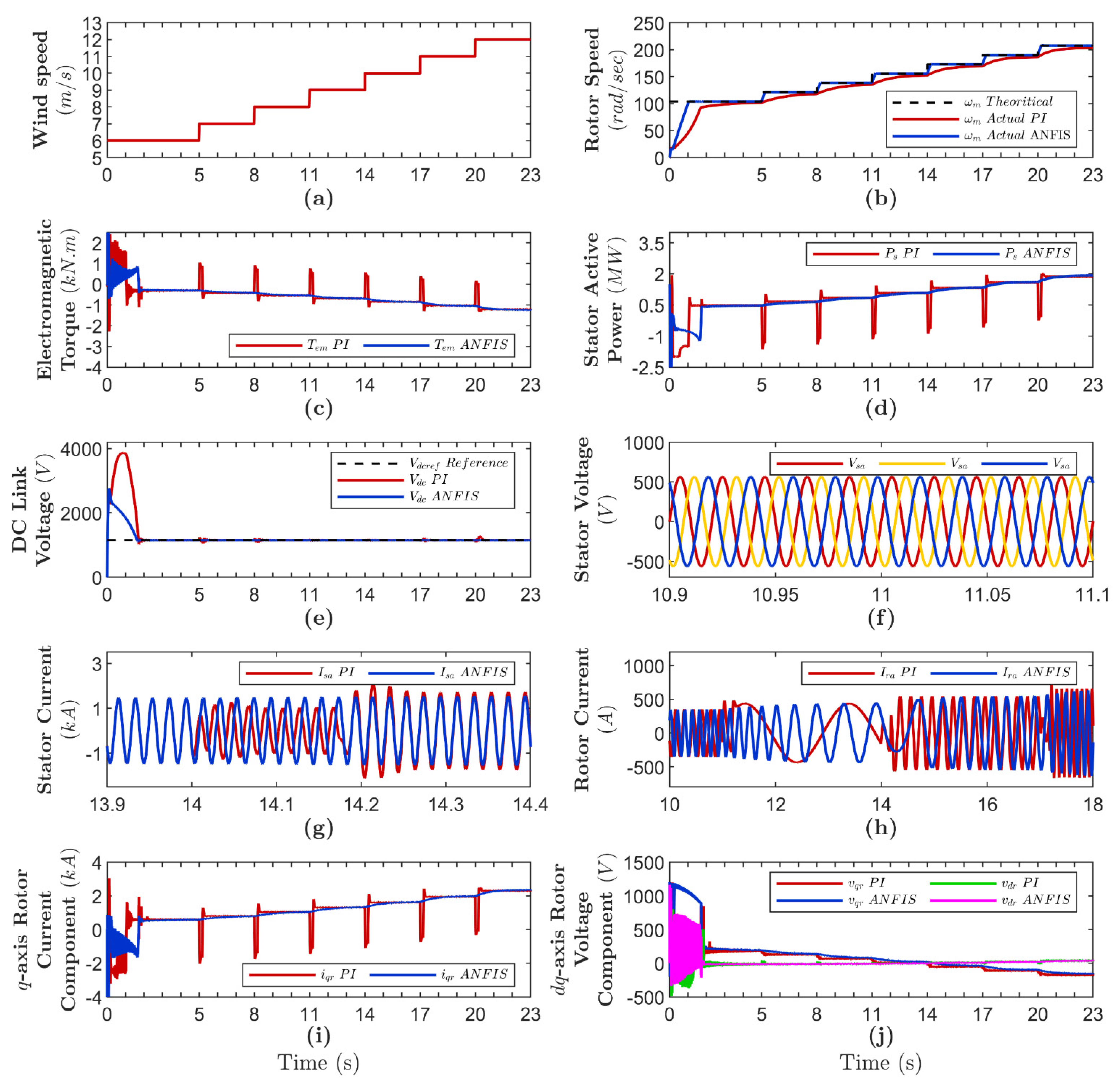
5.1. Case-I: Step Increase in Input Wind Speed

In this case, the input wind speed is increased in step manner as shown in Figure 12a and according to data presented in Table 5. The rotor speed tracking of conventional control and the proposed controller is shown in Figure 12b. There was a significant difference in rotor speed response. The electromagnetic torque response is shown in Figure 12c. The stator active power is observed in Figure 12d. Figure 12e and f present the DC-link voltage and stator voltage response, respectively.

The single a-phase stator current response comparison during step wind speed change at t = 14 s from 9 m/s to 10 m/s is shown in Figure 12g. The proposed controller stator current response remains sinusoidal without any swell condition in current, whereas; the conventional controller shows the unbalance operation. Figure 12h shows the single a-phase rotor current response comparison. It can be observed at t = 14 and 17 s when wind speed increase occurs. The conventional controller shows an unbalance operation along with overshoot. The quadrature axis current component of rotor side converter ($i_{qr}$) response is shown in Figure 12i. Whenever there is wind speed increase operation, the proposed controller shows a smooth transition, whereas the conventional controller shows oscillation at each change instant. The quadrature and direct axis voltage component of the rotor side converter is shown in Figure 12j.

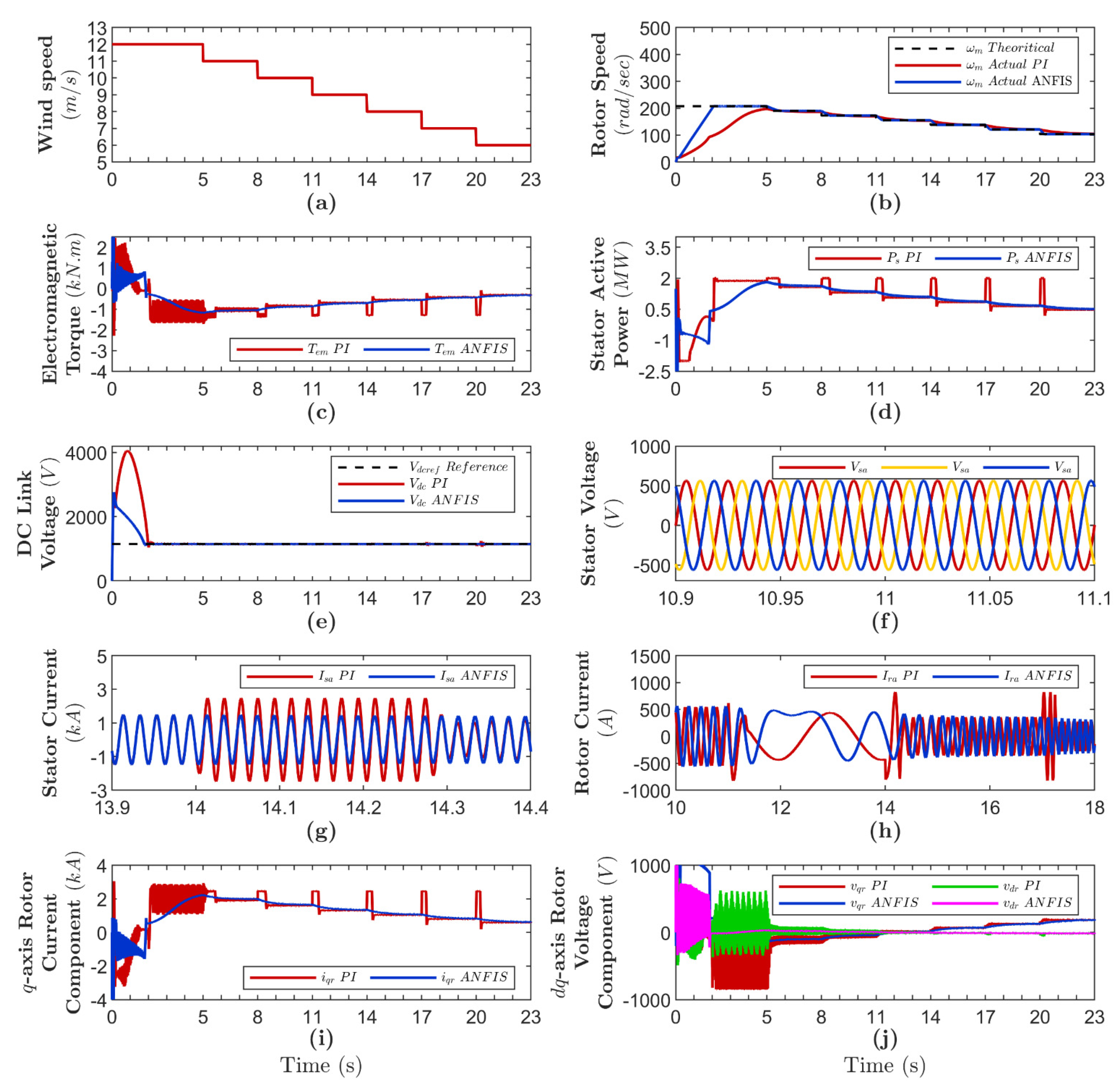
5.2. Case-II: Step Decrease in Input Wind Speed

In this case, the input wind speed is decreased in a step manner, as shown in Figure 13a and according to data presented in Table 5 Case-II. The rotor speed tracking of conventional control and the proposed controller are shown in Figure 13b. The electromagnetic torque response is shown in Figure 13c. The stator active power is observed in Figure 13d. Figure 13e and f present the DC-link voltage and stator voltage response, respectively.

The single a-phase stator current response comparison during step wind speed decrease at t = 14 s from 9 m/s to 8 m/s is shown in Figure 13g. The proposed controller stator current response remains sinusoidal without any swell condition in current whereas, the conventional controller shows current swell. Figure 13h shows the single a-phase rotor current response comparison. It can be observed at t = 10 and 18 s when wind speed decrease occurs, the conventional controller shows unbalanced operation and overshoot. The quadrature axis current component of rotor side converter ($i_{qr}$) response is shown in Figure 13i. Whenever there is a decrease in wind speed operation, the proposed controller shows a smooth transition, whereas the conventional controller shows oscillation at each change instant. The quadrature and direct axis voltage component of the rotor side converter is shown in Figure 13j.

5.3. Case-III: Intermittent Change in Input Wind Speed

In this case, the input wind speed is intermittent and shown in Figure 14a, according to data presented in Table 5 Case-III. The rotor speed tracking of conventional control and the proposed controller is shown in Figure 14b. The electromagnetic torque response is shown in Figure 14c. The stator active power is observed in Figure 14d. Figure 14e,f present the DC-link voltage and stator voltage response, respectively.

The single a-phase stator current response comparison during step wind speed decrease at t = 8 s from 10 m/s to 9 m/s is shown in Figure 14g. The proposed controller stator current response remains sinusoidal without any swell condition in current, whereas the conventional controller shows the current swell. Figure 14h shows the single a-phase rotor current response comparison. It can be observed at t = 5, 8, 11, and 14 s when wind speed change occurs, and the conventional controller shows unbalance operation along with overshoot. The quadrature axis current component of rotor side converter ($i_{qr}$) response is shown in Figure 14i. Whenever there is a change in wind speed operation, the proposed controller shows smooth transition, whereas the conventional controller shows oscillation at each change instant. The quadrature and direct axis voltage component of the rotor side converter is shown in Figure 14j. The performance comparison of ANFIS and PI controller is presented in

Table 8. Performance comparison of ANFIS and PI controller.

Case Study	Simulation Time Instant (sec)	Wind Speed	Rotor Speed (rad/sec)		Stator Active Power (MW)		Percentage Improvement in Power (%)
			PI	ANFIS	PI	ANFIS
Case-I	4	6	100.6	103.7	0.4786	0.4878	1.89
	7	7	115.9	120.9	0.6261	0.6372	1.74
	10	8	133.4	138.2	0.8386	0.8491	1.24
	13	9	151.1	155.5	1.0562	1.0683	1.13
	16	10	168.2	172.8	1.3150	1.3320	1.28
	19	11	185.4	190.2	1.5860	1.6140	1.73
	22	12	202.5	207.3	1.8830	1.9200	1.93
Case-II	4	12	195.2	207.3	1.7732	1.8740	5.38
	7	11	187.3	190.2	1.5860	1.6380	3.17
	10	10	170.5	172.8	1.3150	1.3620	3.45
	13	9	153.7	155.5	1.0680	1.1120	3.96
	16	8	137.1	138.2	0.8479	0.8894	4.67
	19	7	120.2	120.9	0.6533	0.6928	5.70
	22	6	101.1	103.7	0.4939	0.5236	5.67
Case-III	4	8	129.1	138.2	0.7889	0.8478	6.95
	7	10	165.9	172.8	1.3127	1.3265	1.04
	10	9	153.8	155.5	1.0680	1.0970	2.64
	13	12	199.9	207.3	1.8830	1.9070	1.26
	17	7	120.9	123.4	0.6531	0.7071	7.64

considering rotor speed and stator active power. Considering all three cases, there is 3.28% improvement in stator active power.

In terms of stabilizing the stator power output, the suggested controller outperforms the PI controller. In contrast, the PI solution exhibits power oscillations at speed change instant, while the ANFIS response exhibits smooth tracking.

The voltage reference for the DC-link is 1150 volts. The ANFIS controller DC-link voltage response is constant during operation compared with the ANFIS response; the PI response demonstrates that the DC-link voltage oscillates at the instant of speed change and overshoots at around 3980 volts max, which is 37% greater than the ANFIS response.

6. Conclusions

This paper proposed an ANFIS controller for maximum power extraction from the wind for grid-connected DFIG-based WECS. The controller has implemented an ANFIS controller for peak power point tracking. For training, an ANFIS includes input and target data; in this case, the rotor speed is used as the input data, and the torque reference is used as the target or output data. The proposed controller has implemented a 2 MW variable speed wind turbine in MATLAB/Simulink subject to variable wind speed conditions. The simulation study shows that the proposed ANFIS MPPT controller approach exhibited good dynamic performance and quick response for wind speed change while ensuring peak power point tracking. Comparison analysis with a conventional proportional–integral controller approach showed that the ANFIS approach resulted in smoother power tracking and reduced chattering than the conventional approach with a wide range of wind speed changes. The proposed ANFIS MPPT controller shows a 3.28 percent improvement in stator active power than the proportional–integral controller.

This research may be further explored, taking into consideration the controller with multivariable input. The system’s performance may be improved in the future if the changing pitch angle and the actual power generated are taken into consideration, along with rotor speed. Furthermore, performance may be compared with that of other intelligent controllers.

References

1. Qazi, A.; Hussain, F.; Rahim, N.A.B.D.; Hardaker, G.; Alghazzawi, D.; Shaban, K.; Haruna, K. Towards Sustainable Energy: A Systematic Review of Renewable Energy Sources, Technologies, and Public Opinions. IEEE Access 2019, 7, 63837–63851. [Google Scholar] [CrossRef]
2. Chhipa, A.A.; Vyas, S.; Kumar, V.; Joshi, R.R. Role of Power Electronics and Optimization Techniques in Renewable Energy Systems. In Intelligent Algorithms for Analysis and Control of Dynamical Systems; Kumar, R., Singh, V.P., Akhilesh, M., Eds.; Springer: Singapore, 2021; pp. 167–175. [Google Scholar] [CrossRef]
3. Wang, H.; Di Pietro, G.; Wu, X.; Lahdelma, R.; Verda, V.; Haavisto, I. Renewable and Sustainable Energy Transitions for Countries with Different Climates and Renewable Energy Sources Potentials. Energies 2018, 11, 3523. [Google Scholar] [CrossRef] [Green Version]
4. Chen, Z.; Yin, M.; Zou, Y.; Meng, K.; Dong, Z.Y. Maximum Wind Energy Extraction for Variable Speed Wind Turbines with Slow Dynamic Behavior. IEEE Trans. Power Syst. 2017, 32, 3321–3322. [Google Scholar] [CrossRef]
5. Rodríguez-Amenedo, J.L.; Arnaltes, S.; Rodríguez, M.A. Operation and Coordinated Control of Fixed and Variable Speed Wind Farms. Renew. Energy 2008, 33, 406–414. [Google Scholar] [CrossRef]
6. Portillo, R.C.; Prats, M.Á.M.; Leon, J.I.; Sánchez, J.A.; Carrasco, J.M.; Galván, E.; Franquelo, L.G. Modeling Strategy for Back-to-Back Three-Level Converters Applied to High-Power Wind Turbines. IEEE Trans. Ind. Electron. 2006, 53, 1483–1491. [Google Scholar] [CrossRef]
7. Valenciaga, F.; Puleston, P.F.; Battaiotto, P.E. Variable structure system control design method based on a differential geometric approach: Application to a wind energy conversion subsystem. IEE Proc. Control. Theory Appl. 2004, 151, 6–12. [Google Scholar] [CrossRef]
8. Zhou, F.; Liu, J. A Robust Control Strategy Research on PMSG-Based WECS Considering the Uncertainties. IEEE Access 2018, 6, 51951–51963. [Google Scholar] [CrossRef]
9. Mesemanolis, A.; Mademlis, C.; Kioskeridis, I. Optimal Efficiency Control Strategy in Wind Energy Conversion System with Induction Generator. IEEE J. Emerg. Sel. Top. Power Electron. 2013, 1, 238–246. [Google Scholar] [CrossRef]
10. Akhmatov, V. Variable-Speed Wind Turbines with Doubly-Fed Induction Generators Part III: Model with the Back-to-Back Converters. Wind Eng. 2003, 27, 79–91. [Google Scholar] [CrossRef]
11. Naidu, N.K.S.; Singh, B. Grid-Interfaced DFIG-Based Variable Speed Wind Energy Conversion System with Power Smoothening. IEEE Trans. Sustain. Energy 2017, 8, 51–58. [Google Scholar] [CrossRef]
12. Cheng, M.; Zhu, Y. The State of the Art of Wind Energy Conversion Systems and Technologies: A Review. Energy Convers. Manag. 2014, 88, 332–347. [Google Scholar] [CrossRef]
13. Lin, W.M.; Hong, C.M. Intelligent Approach to Maximum Power Point Tracking Control Strategy for Variable-Speed Wind Turbine Generation System. Energy 2010, 35, 2440–2447. [Google Scholar] [CrossRef]
14. Hosseinzadeh, M.; Salmasi, F.R. Analysis and detection of a wind system failure in a micro-grid. J. Renew. Sustain. Energy 2016, 8, 043301–043317. [Google Scholar] [CrossRef]
15. Tripathi, S.M.; Tiwari, A.N.; Singh, D. Grid-Integrated Permanent Magnet Synchronous Generator Based Wind Energy Conversion Systems: A Technology Review. Renew. Sustain. Energy Rev. 2015, 51, 1288–1305. [Google Scholar] [CrossRef]
16. Abdullah, M.A.; Yatim, A.H.M.; Tan, C.W.; Saidur, R. A Review of Maximum Power Point Tracking Algorithms for Wind Energy Systems. Renew. Sustain. Energy Rev. 2012, 16, 3220–3227. [Google Scholar] [CrossRef]
17. Kumar, D.; Chatterjee, K. A Review of Conventional and Advanced MPPT Algorithms for Wind Energy Systems. Renew. Sustain. Energy Rev. 2016, 55, 957–970. [Google Scholar] [CrossRef]
18. Apata, O.; Oyedokun, D.T.O. An Overview of Control Techniques for Wind Turbine Systems. Sci. Afr. 2020, 10, e00566. [Google Scholar] [CrossRef]
19. Lalouni, S.; Rekioua, D.; Idjdarene, K.; Tounzi, A. Maximum Power Point Tracking Based Hybrid Hill-Climb Search Method Applied to Wind Energy Conversion System. Electr. Power Compon. Syst. 2015, 43, 1028–1038. [Google Scholar] [CrossRef]
20. Hua, A.C.-C.; Cheng, B.C.-H. Design and Implementation of Power Converters for Wind Energy Conversion System. In Proceedings of the 2010 International Power Electronics Conference—ECCE ASIA, Sapporo, Japan, 21–24 June 2010; pp. 323–328. [Google Scholar] [CrossRef]
21. Femia, N.; Granozio, D.; Petrone, G.; Spagnuolo, G.; Vitelli, M. Predictive Amp; Adaptive MPPT Perturb and Observe Method. IEEE Trans. Aerosp. Electron. Syst. 2007, 43, 934–950. [Google Scholar] [CrossRef]
22. Urtasun, A.; Sanchis, P.; San Martín, I.; López, J.; Marroyo, L. Modeling of Small Wind Turbines Based on PMSG with Diode Bridge for Sensorless Maximum Power Tracking. Renew. Energy 2013, 55, 138–149. [Google Scholar] [CrossRef] [Green Version]
23. Xia, Y.; Ahmed, K.H.; Williams, B.W. Wind Turbine Power Coefficient Analysis of a New Maximum Power Point Tracking Technique. IEEE Trans. Ind. Electron. 2013, 60, 1122–1132. [Google Scholar] [CrossRef]
24. Abdullah, M.A.; Yatim, A.H.M.; Tan, C.W. An Online Optimum-Relation-Based Maximum Power Point Tracking Algorithm for Wind Energy Conversion System. In Proceedings of the 2014 Australasian Universities Power Engineering Conference, AUPEC 2014—Proceedings, Perth, WA, Australia, 28 September–1 October 2014. [Google Scholar] [CrossRef]
25. Bendib, B.; Belmili, H.; Krim, F. A Survey of the Most Used MPPT Methods: Conventional and Advanced Algorithms Applied for Photovoltaic Systems. Renew. Sustain. Energy Rev. 2015, 45, 637–648. [Google Scholar] [CrossRef]
26. Hosseini, S.H.; Farakhor, A.; Haghighian, S.K. Novel Algorithm of Maximum Power Point Tracking (MPPT) for Variable Speed PMSG Wind Generation Systems through Model Predictive Control. In Proceedings of the ELECO 2013—8th International Conference on Electrical and Electronics Engineering, Bursa, Turkey, 28–30 November 2013; pp. 243–247. [Google Scholar] [CrossRef]
27. Yu, K.N.; Liao, C.K. Applying Novel Fractional Order Incremental Conductance Algorithm to Design and Study the Maximum Power Tracking of Small Wind Power Systems. J. Appl. Res. Technol. 2015, 13, 238–244. [Google Scholar] [CrossRef] [Green Version]
28. Hohm, D.P.; Ropp, M.E. Comparative Study of Maximum Power Point Tracking Algorithms. Prog. Photovolt. Res. Appl. 2003, 11, 47–62. [Google Scholar] [CrossRef]
29. Pagnini, L.C.; Burlando, M.; Repetto, M.P. Experimental Power Curve of Small-Size Wind Turbines in Turbulent Urban Environment. Appl. Energy 2015, 154, 112–121. [Google Scholar] [CrossRef]
30. Hilloowala, R.M.; Sharaf, A.M. A Rule-Based Fuzzy Logic Controller for a PWM Inverter in a Stand Alone Wind Energy Conversion Scheme. IEEE Trans. Ind. Appl. 1996, 32, 57–65. [Google Scholar] [CrossRef]
31. Galdi, V.; Piccolo, A.; Siano, P. Designing an Adaptive Fuzzy Controller for Maximum Wind Energy Extraction. IEEE Trans. Energy Convers. 2008, 23, 559–569. [Google Scholar] [CrossRef]
32. Galdi, V.; Piccolo, A.; Siano, P. Exploiting Maximum Energy from Variable Speed Wind Power Generation Systems by Using an Adaptive Takagi-Sugeno-Kang Fuzzy Model. Energy Convers. Manag. 2009, 50, 413–421. [Google Scholar] [CrossRef]
33. Ata, R. Artificial Neural Networks Applications in Wind Energy Systems: A Review. Renew. Sustain. Energy Rev. 2015, 49, 534–562. [Google Scholar] [CrossRef]
34. Thongam, J.S.; Bouchard, P.; Ezzaidi, H.; Ouhrouche, M. Artificial Neural Network-Based Maximum Power Point Tracking Control for Variable Speed Wind Energy Conversion Systems. In Proceedings of the IEEE International Conference on Control Applications, St. Petersburg, Russia, 8–10 July 2009; pp. 1667–1671. [Google Scholar] [CrossRef]
35. Patyra, M.J.; Grantner, J.L.; Koster, K. Digital Fuzzy Logic Controller: Design and Implementation. IEEE Trans. Fuzzy Syst. 1996, 4, 439–459. [Google Scholar] [CrossRef]
36. Jang, J.-S.R. ANFIS: Adaptive-Network-Based Fuzzy Inference System. IEEE Trans. Syst. Man. Cybern. 1993, 23, 665–685. [Google Scholar] [CrossRef]
37. Abad, G.; López, J.; Rodríguez, M.A.; Marroyo, L.; Iwanski, G. Doubly Fed Induction Machine: Modeling and Control for Wind Energy Generation; Institute of Electrical and Electronics Engineers: Piscataway, NJ, USA, 2011. [Google Scholar] [CrossRef]
38. Biswas, D.; Sahoo, S.S.; Tripathi, P.M.; Chatterjee, K. Maximum Power Point Tracking for Wind Energy System by Adaptive Neural-Network Based Fuzzy Inference System. In Proceedings of the 2018 4th International Conference on Recent Advances in Information Technology (RAIT), Dhanbad, India, 15–17 March 2018; pp. 1–6. [Google Scholar] [CrossRef]
39. Asghar, A.B.; Liu, X. Adaptive Neuro-Fuzzy Algorithm to Estimate Effective Wind Speed and Optimal Rotor Speed for Variable-Speed Wind Turbine. Neurocomputing 2018, 272, 495–504. [Google Scholar] [CrossRef]
40. Kumar, A.; Giribabu, D. Performance Improvement of DFIG Fed Wind Energy Conversion System Using ANFIS Controller. In Proceedings of the 2016 2nd International Conference on Advances in Electrical, Electronics, Information, Communication and Bio-Informatics (AEEICB), Chennai, India, 27–28 February 2016; pp. 202–206. [Google Scholar] [CrossRef]
41. Mathworks. Available online: https://www.mathworks.com/products/hdl-coder.html (accessed on 21 August 2021).
Figure 1. Grid-connected DFIG-based WECS configuration.
Energies 14 06275 g001
Figure 2. Block diagram of RSC vector control of the DFIG.
Energies 14 06275 g002
Figure 3. The architecture of the ANFIS controller.
Energies 14 06275 g003
Figure 4. Block diagram of ANFIS MPPT control.
Energies 14 06275 g004
Figure 5. The architecture of the developed ANFIS-based MPPT controller.
Energies 14 06275 g005
Figure 6. Initial input speed membership functions for training.
Energies 14 06275 g006
Figure 7. Neural network tuned input speed membership functions.
Energies 14 06275 g007
Figure 8. Step size during the training.
Energies 14 06275 g008
Figure 9. Step size during the training.
Energies 14 06275 g009
Figure 10. Power and rotor speed characteristics of WT at different wind speed.
Energies 14 06275 g010
Figure 11. C p λ i characteristics with variation in pitch angle (β).
Energies 14 06275 g011
Figure 12. Simulated response under step wind speed increase: (a) input wind speed, (b) rotor speed, (c) electromagnetic torque, (d) stator active power, (e) DC-link voltage, (f) stator voltage, (g) stator current of a-phase, (h) rotor current of a-phase, (i) q-axis rotor current component, and (j) d and q axis rotor voltage component.
Energies 14 06275 g012
Figure 13. Simulated response under step wind speed decrease: (a) Input wind speed. (b) Rotor speed. (c) Electromagnetic torque. (d) Stator active power. (e) DC-link voltage. (f) Stator voltage. (g) Stator current of a-phase. (h) Rotor current of a-phase. (i) q-axis rotor current component. (j) d and q axis rotor voltage component.
Energies 14 06275 g013
Figure 14. Simulated response under step increase wind speed: (a) input wind speed, (b) rotor speed, (c) electromagnetic torque, (d) stator active power, (e) DC-link voltage, (f) stator voltage, (g) stator current of a-phase, (h) rotor current of a-phase, (i) q-axis rotor current component, and (j) d and q axis rotor voltage component.
Energies 14 06275 g014