The Impact of Environmental Policy Stringency on Renewable Energy Production in the Visegrad Group Countries

Abstract

Various environmental policy instruments supporting the development of renewable energy are used on an increasing scale as part of the policy of mitigating climate change and more. In our paper, we examine the influence of environmental policy stringency on renewable energy production in the Czech Republic, Hungary, Poland and Slovakia for the period 1993–2012 after controlling for gross domestic product per capita growth, CO₂ emissions per capita and income inequality. We use the Panel Pooled Mean Group Autoregressive Distributive Lag model to analyze the long-run and the short-run relationship between restrictiveness of environmental policy and renewable energy generation. The results reveal that, in the long run, a more stringent environmental policy has a positive impact both on the increase in the absolute volume of renewable energy production, as well as on the replacement of energy from fossil sources. Our main findings indicate that renewable energy production is positively influenced not only by the stringency of instruments aimed directly at the development of this energy sector, but also by the stringency of instruments with other environmental goals and by the overall level of restrictiveness of the environmental policy.

1. Introduction

Renewables play a growing role in energy mixes around the world [1]. The deployment of renewable energy has increased in recent years, especially in EU countries and US states [2]. Replacing fossil fuels with renewable energy sources not only contributes to the decrease in carbon dioxide (CO₂) emissions, but also to the reduction of emissions of other air pollutants, such as nitrogen oxides (NO_X) and sulfur oxides (SO_x). Renewable energy is a major element for the desired move towards low carbon economies [3]. Investing in renewable energy can, in addition to environmental benefits, contribute to greater energy security in the face of uncertain fossil fuel markets [4].

Due to the production cost gap between renewable energy and fossil fuel energy, it is necessary to support the development of renewable energy through an appropriate environmental policy. Public policies supporting the development of renewable energy have been used in developed economies since 1980 and, since 2000, in an increasing number of emerging countries [5]. Although, currently, in some countries, the cost of producing renewable energy is lower than that of conventional energy (e.g., in Australia, in the case of solar and wind energy [6]), the government support policy in these countries is still applied. Environmental policies aiming at promoting renewable energy include fiscal and financial incentives, regulatory measures and strategy planning. Among these instruments, the most commonly used globally at state/provincial or national level are feed-in tariffs and renewable portfolio standards [7]. Whether these various environmental (support) policy instruments are effective in promoting the development of renewable energy remains an open question. The results of empirical research in this regard bring contradictory conclusions (e.g., [2,5,8,9,10,11]).

The literature more and more often emphasizes that, in the proper assessment of the effectiveness of environmental policy instruments in supporting renewable energy, it is necessary to take into account not only the fact of introducing a given instrument or not, but most of all the design features that characterize these instruments, such as their scope, flexibility, monitoring, or stringency [4,11,12,13,14,15,16]. In practice, environmental policy instruments differ significantly and taking into account the differences in their design features allows us to understand which aspects of the environmental policy are the most important to achieve the environmental objectives set.

It should be noted that the use of renewable energy may be influenced not only by environmental policy instruments directly aimed at its development, but also by instruments aimed at achieving other environmental goals, such as reduction of CO₂, SO_x or NO_x. In general, renewable energy is widely viewed as an environmentally friendly energy type and, in countries where the overall stringency level of environmental policy is high, there may be strong incentives to develop renewable energy.

The aim of our paper is to examine the influence of environmental policy stringency on renewable energy production in the Czech Republic, Hungary, Poland and Slovakia for the period 1993–2012 after controlling for gross domestic product (GDP) per capita growth, CO₂ emissions per capita and income inequality (measured by the Gini index).

The Czech Republic, Hungary, Poland and Slovakia that make up the Visegrad Group, are former socialist countries that have undergone economic transformation since the early 1990s. Energy production in these countries is based, to a large extent (the Czech Republic, Hungary, Slovakia), or very much (Poland), on the use of fossil fuels. The natural conditions for investing in renewable energy sources in the Visegrad Group countries are generally moderately positive, taking into account regional differences with regard to specific renewable technologies (e.g., Slovakia has favorable conditions especially for the development of hydropower and Hungary for the development of geothermal energy). Since the accession of the Visegrad Group countries to the European Union (i.e., since 2004), their national environmental policies have been largely influenced by the policy of the EU.

In our paper, we focus on the impact of the overall level of environmental policy stringency and the restrictiveness of individual instruments of this policy, i.e., taxes, standards and subsidies. Our study contributes to the literature in that, to the best of our knowledge, the importance of a general (aggregate) level of environmental policy restrictiveness for boosting renewable energy has not yet been investigated. Secondly, we examine the stringency impact of both environmental policy instruments that are directly related to renewable energy (i.e., government subsidies for renewable energy technologies), as well as the stringency impact of two types of these instruments (i.e., taxes and standards), targeting other environmental objectives, such as reducing CO₂, NO_x, SO_x and particulate matter emissions. Previous literature examined the effectiveness of only instruments devoted directly to promoting the use of renewable energy or mitigating climate change due to reducing CO₂ emissions.

The rest of the paper is organized as follows: Section 2 discusses the stringency of environmental policy in terms of its measuring and economic and environmental impact. Section 3 presents the literature review on the impact of environmental policy instruments on renewable energy and on the control variables used in our models. The materials and research method are discussed in Section 4. Section 5 shows the results of our research and Section 6 provides the discussion and conclusions for environmental policy implications for renewable energy development.

2. Environmental Policy Stringency and its Impact on the Economy and the Natural Environment

One of the features of environmental policy—and public policy in general—is its stringency, alongside efficiency, effectiveness, flexibility, acceptability and distributive fairness. Environmental policy stringency is ‘the strength of the environmental policy signal—the explicit or implicit cost of environmentally harmful behavior, for example, pollution’ [17] (p. 3). On the other hand, in the case of environmental policy instruments in the form of subsidies that reward environmentally friendly behavior (such as tax reliefs and tax exemptions related to environmental protection, feed-in tariffs for renewable energy), higher subsidies are interpreted as more stringent environmental policies, because they increase the opportunity cost of pollution, thus giving an advantage to ‘cleaner’ activities [18] (p. 14).

The stringency of environmental policy can be assessed using various measures, such as survey indicators, variables measuring pollution abatement efforts, direct assessments of regulations, measures based on ambient pollution, emissions, or energy use and composite indexes [19,20]. Survey indicators are constructed on the basis of the subjective opinions and perceptions of various respondents (most often managers) on the severity of the environmental protection instruments used in a given country. An example of such a survey-based measure is the indicator of the stringency of environmental regulations developed by the World Economic Forum, obtained from the responses of the Executive Opinion Survey [20]. Indicators relating to abatement efforts include measures of both private and public efforts to control pollution, e.g., pollution abatement costs, governmental environmental R&D expenditures and revenues from environmental taxes. Using direct assessments of regulations at the sector or country level is a difficult task due to the multidimensionality and simultaneity of adopted (abolished) environmental policy instruments. Examples of these indicators include the lead content of gasoline or standardized air quality limits used to measure the overall severity of environmental regulations. Measures based on ambient pollution, emissions, or energy use include information on the level of (or the change in) emissions and energy use at the country or sector level, totally or per capita. Composite indexes may be constructed simply from counts of regulations, non-governmental environmental organizations, international treaties signed or based on statistical aggregation techniques using a set of environmental policy indicators [19].

One of the latter is the environmental policy stringency (EPS) index developed by the OECD, which is used more and more frequently in the assessment of the restrictiveness of environmental policy. The EPS index is created by aggregating information on selected environmental policy instruments, mainly related to the climate and air pollution. It is a weighted average of the stringency of individual environmental policy instruments, divided into market instruments (environmental taxes, emission trading systems, feed-in tariffs) and non-market instruments (emission standards, government subsidies for renewable energy technologies). The instruments are scored on a 0–6 scale increasing in stringency. A detailed description of the calculation of the EPS index can be found in the study by Botta and Koźluk [18]. The EPS index ensures that the stringency of environmental policies in different countries is comparable across countries.

The tightening of environmental regulations is considered in the environmental economics literature in the context of the Porter hypothesis and the pollution haven hypothesis. According to the former, the tightening of environmental requirements may contribute to the improvement of the competitiveness of enterprises by encouraging them to seek and implement widely understood ecological innovations. Eco-innovation can reduce costs, increase productivity and create new market opportunities. Companies that are the first to implement innovative environmental solutions on the market may benefit in particular [21]. According to the pollution haven hypothesis, differences in strict environmental policies can result in the relocation of highly polluting industries from industrialized economies to jurisdictions with very lax or no environmental regulations [22,23].

The tightening of environmental policy has its economic and environmental consequences. The stringency of environmental regulations encourages market development for equipment designed for pollution abatement and prevention and it affects countries’ specialization in exports of environmental products and technologies [24]. In addition, more restrictive environmental policies are related to the loss of competitiveness in the most polluting sectors and a decline in their export. Simultaneously, they contribute to the emergence of a comparative advantage and export growth in ‘cleaner’ industries [25]. Sung and Song [26] examined how environmental policy stringency influences the export performance of the bioenergy technology sector in the short and long run using panel data over the period 1995–2012 for 16 OECD countries. They found a positive impact of the strength of environmental policy on exports in both the short and long run.

Ahmed and Ahmed found that stringent environmental policies have a negative impact on China’s GDP [27]. Bigerna et al. [28] analyzed the strength of environmental regulation on efficiency in the electricity sector for a panel of European Union countries and argued that stringent policy negatively affects productivity. The study by Wang et al. [29] based on the panel data of OECD countries indicates that, within a certain level of stringency, the environmental policy has a positive impact on green productivity growth which supports the Porter hypothesis. However, after exceeding a certain level of stringency, as the compliance cost effect is higher than innovation offset effect, the impact of environmental policy on green productivity growth turns to be adverse. On the other hand, the other OECD-based study by Albrizio et al. [30] reveals that, at the industry-level, the growing restrictiveness of environmental policy results in a short-term increase in productivity growth in industry in the most technologically advanced countries. However, this tendency is weakened, with the distance from the global limit of productivity. At the firm-level, the most productive companies experience a temporary increase in productivity, while the less productive ones experience a slowdown in productivity.

Rubashkina et al. [31] used pollution abatement and control expenditures as a proxy of environmental policy stringency in their study on the impact of environmental regulation on European manufacturing sectors. Their findings reveal a positive impact of the restrictive environmental policy on innovation activity, as proxied by patents, and no impact on productivity of analyzed sectors. Similar conclusions about the positive role of environmental policy stringency on innovations in environment-related technology were drawn by Johnstone et al. [32]. The results of the research by Galeotti et al. [19] concerning selected OECD countries also confirm the positive, but small impact of environmental policy stringency on environmental innovations and on energy efficiency.

Concerning the empirical studies on the relationship between stringency of environmental policy and environmental quality, their conclusions are not unequivocal. Some scholars claim that a restrictive environmental policy is effective in reducing CO₂ emissions [27,33,34,35,36], SO_x emissions [35,37,38] and NO_X emissions [35]. According to Dong et al. [39], stringent environmental legislation may reduce the number and growth rate of intensively polluting companies in highly regulated regions, especially those operating in heavy industry, due to increased financing costs. On the other hand, the findings by Alexandersson [40] and Godawska [37] indicate that the tightening of the environmental policy has no significant impact on CO₂ emissions. Similarly, Wang et al. [35] found that more restrictive environmental policy does not lead to mitigated PM 2.5 emissions. Sadik-Zada and Ferrari [23] argue that different levels of environmental policy stringency in national states, along with trade openness, lead to carbon leakage which confirms the pollution haven hypothesis.

3. Literature Review

3.1. Impact of Environmental Policy Instruments on Renewable Energy

A growing number of studies take into account the impact of various environmental policy instruments on different aspects of deployment of renewable energy technologies, including renewable energy capacity [2,5,7,8,10,11,14,41,42,43], the development of the renewable energy market [12,44], the contribution of renewables to energy supply [9], renewable energy generation [45], innovations in renewable energy technologies [4,46], societal cost [47,48], the price of power generated [49,50], market value of renewables [51], renewable energy investment risk and return [16,52], energy access [53], employment impact [53,54] and the development of renewable energy technologies [55]. Regarding the role of support policies in promoting renewable energy, the studies yield mixed results, depending on the analyzed period and countries, as well as the types of policy instruments and sources of renewable energy. An important research question analyzed in research on environmental policy instruments is whether quantity (e.g., renewable portfolio standards, auctions) or price-based instruments (e.g., feed-in-tariffs, taxes, grants) are more effective in promoting renewable energy. However, this issue remains unresolved.

Menz and Vachon [8] analyzed five state policy instruments in terms of their contribution to the development of wind energy, taking into account 39 states in the USA over the period 1998–2003. The instruments examined included renewable portfolio standards, mandatory green power offering, fuel generation disclosure rules, public benefits funds and retail choice. Only the first two of them turned out to be significantly and positively related to the development of wind energy.

A more recent study by Bersalli et al. [5], based on panel data for 20 Latin American and 30 European countries over the period 1995–2015, confirms a positive and significant impact of feed-in tariffs, auctions and renewable portfolio standards on the renewable energy capacity in both regions. The effectiveness of these instruments appears to be stronger in Europe than in Latin America, which may be partly related to the different timing of implementing policy instruments (i.e., earlier in Europe than in Latin America). However, tax incentives proved to be insufficient to boost investment in renewable energy sources and, according to Bersalli et al., countries should not base their support policy solely on such instruments [5] (p. 9). Their conclusion on the effectiveness of tax incentives differs from that resulting from the previous study by Kilinc-Ata [2], who found these instruments alongside feed-in-tariffs and tenders to stimulate an increase in the capacity of renewable energy sources. On the other hand, the quota (the renewable portfolio standard) turned out to be ineffective in promoting renewable energy deployment in the 27 EU countries and 50 US states (taking into account the period 1990–2008) [2].

Some scholars [9,10], pointing to the failure of certain support policy instruments, see the reason for this in the uncertainty and high risk for investors and the likelihood of discontinuation of support. Similarly, Polzin et al. [16] argue that feed-in tariffs, auctions and renewable portfolio standards are most effective when reducing the risk of a renewable energy project while increasing return.

Johnstone et al. [4] examined the impact of different instruments of environmental policy on technological innovation in renewable energy sources on a panel of 25 countries using data on patent counts. They concluded that the effectiveness of alternative instruments depends on the type of renewable energy technologies. Broad-based policies (e.g., tradable energy certificates) are more likely to spur technology innovations in the sources that have reached or are approaching competitiveness with fossil fuel sources, such as wind power. Conversely, to stimulate innovation in more expensive renewable energy technologies such as solar energy, more targeted subsidies such as feed-in tariffs may be required.

Very few studies have examined the role of stringent environmental policy in the development of renewable energy. They focused exclusively on individual types of policy instruments, such as renewable portfolio standards [11,12] and feed-in-tariffs [14]. To the best of our knowledge, the impact of a general (aggregate) level of environmental policy restrictiveness on renewable energy production has not yet been investigated.

Yin and Powers [11] examined the effectiveness of renewable portfolio standard policies in terms of generating renewable energy capacity employing their own developed policy stringency measure. This measure takes into account several key design features which affect the effectiveness of renewable portfolio standards—nominal requirements of renewable energy amount, coverage (entities required to comply with standards) and allowing or not allowing existing renewable energy capacities to be taken into account in meeting the standards. The study was based on panel data for 50 US states between 1993 and 2006. The results revealed that the higher stringency of renewable portfolio standards, the larger in-state renewable energy development. This positive impact of renewable portfolio standards can be weakened by allowing trade of renewable energy credits within these policies. Yin and Powers stress the need to take into account the heterogeneity among renewable portfolio standard policies in order to obtain reliable research results on the effectiveness of these policies.

Carley et al. [12] analyzed how changes in state renewable portfolio standard policies relate to the growth of renewable energy markets in the United States from 1992 to 2014. Their study reveals that a one-point increase in these standards’ stringency leads to increases of 0.2%, 1% and 0.3% in the percentage of renewable energy in the electricity generation mix, solar generation and renewable energy capacity, respectively. They measured the stringency of renewable portfolio standards as the amount of renewable energy growth required over the number of years that the policy is in place times the total applicable electricity load.

Jenner et al. [14] assessed the policy strength of price-based instruments, i.e., feed-in-tariffs, using their own developed indicator that takes into account variability in tariff size, contract duration, digression rate, electricity wholesale price and production cost. Their research was based on data from 26 countries of the European Union for the years 1992–2008. They found evidence that feed-in tariffs are effective in boosting solar photovoltaic energy capacity growth. However, this effect is on the high side without taking country characteristics into account and may not be observed without considering the stringency of each policy at all. They concluded that the proper design of the support policy, together with the market context, is more important for the development of renewable energy than the mere implementation of the policy.

3.2. Control Variables

We use control variables such as per capita gross domestic product growth, per capita carbon dioxide emissions and the Gini index as a measure of income inequality to investigate the relationship between the stringency of environmental policy and renewable energy production in order to obtain robust empirical findings.

Scientists have often examined the relationship between gross domestic product and the production (or consumption) of renewable energy and have found contradicting results. The belief that higher GDP is correlated with greater use of renewable energy is based on the assumption that higher income means more resources available to implement and promote costly sustainable environmental alternatives, including greater deployment of renewables [56]. The correctness of the view about the positive impact of GDP on renewable energy consumption (supply) was confirmed by many scholars who researched GDP per capita [57,58,59,60,61,62,63,64] or GDP in absolute terms [65]. In addition, Przychodzen and Przychodzen [66], using data from 27 transition countries over the years 1990–2014 have found that higher GDP growth stimulate renewable energy generation. Kilinc-Ata [2] have reached the same conclusion when considering a 1990–2008 panel dataset of 27 EU countries and 50 US states and renewable energy capacity. However, several authors have found results that reject the hypothesis of a positive influence of GDP on renewable energy consumption, indicating a negative impact of GDP [67,68] or the insignificance of this impact [9,42,69,70].

CO₂ emissions are, as well as GDP, often analyzed in the literature as a factor influencing the deployment of renewable energy. High CO₂ emissions can lead to striving for a cleaner environment and restraining the climate change; consequently, they encourage the deployment of renewable energy, especially in countries with an ambitious climate policy and committed to a significant reduction of CO₂ emissions. Emitting more CO₂ can mean a greater incentive to invest in renewable energy. Omri et al. [64] examined the drivers of renewable energy consumption for a panel of 64 countries between 1990 and 2011, including high-, middle- and low-income countries. They found that CO₂ emissions per capita have a statistically significant impact on the per capita renewable energy consumption, regardless of the level of GDP. Other studies also support the view that increasing CO₂ emissions will enhance the consumption of renewable energy [9,57,69,71,72]. However, Marques et al. [56] and Przychodzen and Przychodzen [66] came to the opposite conclusion. The findings of the former [56], based on panel data for 24 European countries in the years 1990–2006, indicate that CO₂ emissions restrain renewable energy supply. The latter [66], using more recent data (1990–2015) for 27 transition economies, found that the increase in CO₂ emissions per capita reduces the production of energy from renewable sources. In contrast, research on determinants of renewable energy consumption in Malaysia considering data for 1980–2015 [73] reveal no significant impact of CO₂ emissions on renewable energy. Bayar et al. [74] found a unilateral causality from CO₂ emissions to renewable energy in Lithuania and Slovenia and a reciprocal causality between renewable energy and CO₂ emissions in Romania and Slovakia; however, they discovered no such effects in case of the other seven analyzed EU transition economies in the years 1995–2015.

Growing income inequality is a fact both in most developed countries [75] and in post-socialist countries undergoing transformation, such as the Visegrad Group countries [76]. Some empirical studies indicate that higher income inequality is associated with less environmental degradation [77,78] and suggest that there might be a trade-off between reducing income inequality and improving environmental quality. McGee and Greiner [79] found that nations less interested in pursuing the reduction in income inequality are likely to encourage crowding out fossil fuel energy use by deploying privately installed and distributed renewable energy production technologies. According to Wu and Xie [80] higher income inequality favors emission reductions in OECD and non-OECD high-income countries, while this impact is insignificant in low-income non-OECD countries in the long run. Investing in renewable energy sources is costly and requires capital accumulation and investors with a sufficiently high level of income. However, there are also studies showing the influence of reducing income inequality on the decrease in CO₂ emissions [81,82], improving air quality [83] and enhancing renewable energy consumption [69]. One possible explanation for this relationship is that the propensity to pollute the environment and to exploit resources exhaustively is greater among people with low incomes, who have to meet their basic living needs at the expense of the environment. Therefore, narrowing income gap leads to an improvement in quality of the environment [82].

4. Materials and Methods

In the paper, we used a balanced annual panel data for the years 1993–2012 collected from OECD and World Bank databases. The length of the series was limited by its availability (the environmental policy stringency index for the Visegrad Group countries is available only up to 2012).

Table 1. Description of variables used in models.

Variables	Definitions	Sources
Dependent variables
RE_P	contribution of renewable energy to total primary energy supply in thous. toe	OECD
RE_S	contribution of renewable energy to total primary energy supply in %	OECD
Independent variable
EPS	environmental policy stringency index	OECD
TAX	environmental taxes stringency	OECD
STAND	emission standards stringency	OECD
SUBS	government subsidies for renewable energy technologies stringency	OECD
Control variables
GDP	GDP per capita growth (annual %)	World Bank
CDIO	CO2 emissions (metric tons per capita)	World Bank
GINI	Gini index	World Bank

presents the definitions of the variables and data sources.

Since the analyzed data were stationary at different levels (I(0) and I(1) but not I(2)), we decided to use the Panel Pooled Mean Group Autoregressive Distributive Lag model for estimation of the long-run and the short-run coefficients (PMG-ARDL estimator). In our research study, we followed the methodology used by Wolde-Rufael and Weldemeskel [33]. To investigate the impact of overall environmental policy stringency on production of renewable energy (in thousand tons of oil equivalent), we estimated the following panel model (first model):

$$\mathrm{RE}\_{\mathrm{P}}_{\mathrm{i},\mathrm{t}}={\mathsf{\alpha }}_{\mathrm{i},\mathrm{t}}+{\mathsf{\beta }}_1{\mathrm{EPS}}_{\mathrm{i},\mathrm{t}}+{\mathsf{\beta }}_2{\mathrm{GDP}}_{\mathrm{i},\mathrm{t}}+{\mathsf{\beta }}_3{\mathrm{CDIO}}_{\mathrm{i},\mathrm{t}}+{\mathsf{\beta }}_4{\mathrm{GINI}}_{\mathrm{i},\mathrm{t}}+{\mathsf{\epsilon }}_{\mathrm{i},\mathrm{t}}$$

(1)

where all variables are logarithms of the data presented in Table 1, i represents countries (1,…,N) and t represents time (1,…,T).

In order to investigate the impact of the overall environmental policy stringency on the total share of renewable energy in total energy production, we estimated the following panel model (second model):

$$\mathrm{RE}\_{\mathrm{S}}_{\mathrm{i},\mathrm{t}}={\mathsf{\alpha }}_{\mathrm{i},\mathrm{t}}+{\mathsf{\beta }}_1{\mathrm{EPS}}_{\mathrm{i},\mathrm{t}}+{\mathsf{\beta }}_2{\mathrm{GDP}}_{\mathrm{i},\mathrm{t}}+{\mathsf{\beta }}_3{\mathrm{CDIO}}_{\mathrm{i},\mathrm{t}}+{\mathsf{\beta }}_4{\mathrm{GINI}}_{\mathrm{i},\mathrm{t}}+{\mathsf{\epsilon }}_{\mathrm{i},\mathrm{t}}$$

(2)

where all variables are logarithms of the data presented in Table 1.

The next (third) model analyzes the impact of the stringency of environmental taxes, emission standards and government subsidies for renewable energy on production of renewable energy (in thousands tons of oil equivalent):

$$\mathrm{RE}\_{\mathrm{P}}_{\mathrm{i},\mathrm{t}}={\mathsf{\alpha }}_{\mathrm{i},\mathrm{t}}+{\mathsf{\beta }}_1{\mathrm{TAX}}_{\mathrm{i},\mathrm{t}}+{\mathsf{\beta }}_2{\mathrm{STAND}}_{\mathrm{i},\mathrm{t}}+{\mathsf{\beta }}_3{\mathrm{SUBS}}_{\mathrm{i},\mathrm{t}}+{\mathsf{\beta }}_4{\mathrm{GDP}}_{\mathrm{i},\mathrm{t}}+{\mathsf{\beta }}_5{\mathrm{CDIO}}_{\mathrm{i},\mathrm{t}}+{\mathsf{\beta }}_6{\mathrm{GINI}}_{\mathrm{i},\mathrm{t}}+{\mathsf{\epsilon }}_{\mathrm{i},\mathrm{t}}$$

(3)

where all variables are logarithms of the data presented in Table 1.

The last (fourth) model tests the impact of stringency of environmental taxes, emission standards and government subsidies for renewable energy technologies on the total share of renewable energy in total energy production:

$$\mathrm{RE}\_{\mathrm{S}}_{\mathrm{i},\mathrm{t}}={\mathsf{\alpha }}_{\mathrm{i},\mathrm{t}}+{\mathsf{\beta }}_1{\mathrm{TAX}}_{\mathrm{i},\mathrm{t}}+{\mathsf{\beta }}_2{\mathrm{STAND}}_{\mathrm{i},\mathrm{t}}+{\mathsf{\beta }}_3{\mathrm{SUBS}}_{\mathrm{i},\mathrm{t}}+{\mathsf{\beta }}_4{\mathrm{GDP}}_{\mathrm{i},\mathrm{t}}+{\mathsf{\beta }}_5{\mathrm{CDIO}}_{\mathrm{i},\mathrm{t}}+{\mathsf{\beta }}_6{\mathrm{GINI}}_{\mathrm{i},\mathrm{t}}+{\mathsf{\epsilon }}_{\mathrm{i},\mathrm{t}}$$

(4)

where all variables are logarithms of the data presented in Table 1.

Since the current production of renewable energy and its share in total energy production is autoregressive, we applied the ARDL model (Auto Regressive Distributive Lag):

$$\mathrm{RE}\_{\mathrm{P}}_{\mathrm{i},\mathrm{t}}={\mathsf{\alpha }}_{\mathrm{i}}+{\displaystyle \sum }_{\mathrm{j}=1}^{\mathrm{p}}{\mathsf{\rho }}_{\mathrm{i},\mathrm{j}}\mathrm{RE}\_{\mathrm{P}}_{\mathrm{i},\mathrm{t}-\mathrm{j}}+{\displaystyle \sum }_{\mathrm{j}=0}^{\mathrm{q}}{\mathsf{\gamma }}_{\mathrm{i},\mathrm{j}}{\mathrm{X}}_{\mathrm{i},\mathrm{t}}+{\mathsf{\epsilon }}_{\mathrm{i},\mathrm{t}}$$

(5)

and

$$\mathrm{RE}\_{\mathrm{S}}_{\mathrm{i},\mathrm{t}}={\mathsf{\alpha }}_{\mathrm{i}}+{\displaystyle \sum }_{\mathrm{j}=1}^{\mathrm{p}}{\mathsf{\rho }}_{\mathrm{i},\mathrm{j}}\mathrm{RE}\_{\mathrm{S}}_{\mathrm{i},\mathrm{t}-\mathrm{j}}+{\displaystyle \sum }_{\mathrm{j}=0}^{\mathrm{q}}{\mathsf{\gamma }}_{\mathrm{i},\mathrm{j}}{\mathrm{X}}_{\mathrm{i},\mathrm{t}}+{\mathsf{\epsilon }}_{\mathrm{i},\mathrm{t}}$$

(6)

ECM representation assumes that the long-run coefficients on the explanatory variables (X_i,t) are the same across the units (one vector of beta coefficients for all units). Such a model can be described as follows:

$$\mathrm{RE}\_{\mathrm{P}}_{\mathrm{i},\mathrm{t}}={\mathsf{\alpha }}_{\mathrm{i}}+{\mathsf{\varphi }}_{\mathrm{i}}\mathrm{RE}\_{\mathrm{P}}_{\mathrm{i},\mathrm{t}-1}+{\mathsf{\beta }}^{\prime }{\mathrm{X}}_{\mathrm{i},\mathrm{t}}+{\displaystyle \sum }_{\mathrm{j}=1}^{\mathrm{p}}{\mathsf{\rho }}_{\mathrm{i},\mathrm{j}}^{*}\mathrm{RE}\_{\mathrm{P}}_{\mathrm{i},\mathrm{t}-\mathrm{j}}+{\displaystyle \sum }_{\mathrm{j}=0}^{\mathrm{q}}{\mathsf{\gamma }}_{\mathrm{i},\mathrm{j}}^{*{}^{\prime }}{\mathrm{X}}_{\mathrm{i},\mathrm{t}}+{\mathsf{\epsilon }}_{\mathrm{i},\mathrm{t}}$$

(7)

and

$$\mathrm{RE}\_{\mathrm{S}}_{\mathrm{i},\mathrm{t}}={\mathsf{\alpha }}_{\mathrm{i}}+{\mathsf{\varphi }}_{\mathrm{i}}\mathrm{RE}\_{\mathrm{S}}_{\mathrm{i},\mathrm{t}-1}+{\mathsf{\beta }}^{\prime }{\mathrm{X}}_{\mathrm{i},\mathrm{t}}+{\displaystyle \sum }_{\mathrm{j}=1}^{\mathrm{p}}{\mathsf{\rho }}_{\mathrm{i},\mathrm{j}}^{*}\mathrm{RE}\_{\mathrm{S}}_{\mathrm{i},\mathrm{t}-\mathrm{j}}+{\displaystyle \sum }_{\mathrm{j}=0}^{\mathrm{q}}{\mathsf{\gamma }}_{\mathrm{i},\mathrm{j}}^{*{}^{\prime }}{\mathrm{X}}_{\mathrm{i},\mathrm{t}}+{\mathsf{\epsilon }}_{\mathrm{i},\mathrm{t}}$$

(8)

where:

${\mathsf{\rho }}_{\mathrm{i},\mathrm{j}}^{*{}^{\prime }}=-{\sum }_{\mathrm{l}=\mathrm{j}+1}^{\mathrm{p}}{\mathsf{\rho }}_{\mathrm{i},\mathrm{j}}^{\prime }$, ${\mathsf{\gamma }}_{\mathrm{i},\mathrm{j}}^{*{}^{\prime }}=-{\sum }_{\mathrm{l}=\mathrm{j}+1}^{\mathrm{q}}{\mathsf{\gamma }}_{\mathrm{i},\mathrm{j}}^{\prime }$, p is the order of the model in the dependent variable, q is the order of the model in the explanatory variable, ${\mathrm{X}}_{\mathrm{i},\mathrm{t}}$ is the vector of explanatory variables defined in models 1—4, β is the vector of long-run coefficients, ρ and γ are the short-term coefficients of the lagged dependent and independent variables and $\mathsf{\varphi }$ represents the error-correction term that estimates the speed of adjustment of the dependent variable (this parameter captures adjustment towards long-term equilibrium; to ensure that there is a long-term equilibrium, we make the assumption that ${\mathsf{\varphi }}_{\mathrm{i}}<0$, so there is a cointegration between dependent and independent variables [84,85]).

In order to test if there is a long-run equilibrium relationship among the time series, we used two panel cointegration tests, developed by Pedroni [86] and by Kao [87]. The idea of the Pedroni panel cointegration test is based on an examination of the residuals of a spurious regression performed using I(1) variables. If the variables are cointegrated, then the residuals should be I(0). The Kao panel cointegration test uses a similar approach to the Pedroni test, but allows for cross-section specific intercepts and homogenous coefficients on the first-stage regressors.

We used the Hausman tests to check the correctness of the model specification. The Hausman tests [88] are tests for econometric model misspecification based on a comparison of two different estimators of the model parameters. Heuristically, the key idea is that, when the model is correctly specified, the compared estimators are close to one another, but, when the model is misspecified, the compared estimators are far apart.

5. Results

The descriptive statistics for the data series are reported in

Table 2. Descriptive statistics for variables.

Country	Variables	Obs.	Mean	SD	Min	Max
Czech Republic	RE_S	20	4.863	1.502	3.320	8.540
	RE_P	20	2115.990	677.390	1428.810	3687.910
	EPS	20	1.589	0.916	0.542	2.892
	GDP	20	2.489	2.946	−5.199	6.566
	CDIO	20	11.636	0.664	10.196	12.679
	GINI	20	26.475	0.454	25.800	27.500
	TAX	20	1.850	0.205	1.500	2.250
	STAND	20	2.638	1.877	0.000	4.500
	SUBS	20	1.150	0.366	1.000	2.000
Hungary	RE_S	20	5.505	3.080	3.180	11.950
	RE_P	20	1437.280	777.060	818.400	2952.770
	EPS	20	1.673	0.963	0.520	2.766
	GDP	20	2.267	2.812	−6.555	5.055
	CDIO	20	5.362	0.384	4.377	5.748
	GINI	20	29.411	2.323	27.000	34.700
	TAX	20	1.663	0.690	1.000	3.000
	STAND	20	2.500	1.918	0.250	4.500
	SUBS	20	1.500	0.513	1.000	2.000
Poland	RE_S	20	5.067	1.451	3.740	8.820
	RE_P	20	4860.490	1483.590	3752.800	8609.600
	EPS	20	1.607	0.812	0.875	2.958
	GDP	20	4.435	1.717	1.286	7.120
	CDIO	20	8.207	0.481	7.514	9.199
	GINI	20	34.311	1.649	33.000	38.000
	TAX	20	2.288	0.640	1.500	3.500
	STAND	20	2.700	1.409	1.500	4.500
	SUBS	20	1.350	0.745	1.000	3.000
Slovakia	RE_S	20	4.288	1.855	2.390	8.160
	RE_P	20	764.31	313.27	432.51	1358.68
	EPS	20	1.360	0.784	0.667	3.054
	GDP	20	4.243	3.450	−5.581	10.800
	CDIO	20	7.178	0.609	5.986	8.323
	GINI	20	26.667	1.285	24.700	29.300
	TAX	20	1.975	0.313	1.500	2.500
	STAND	20	1.463	0.745	0.500	2.250
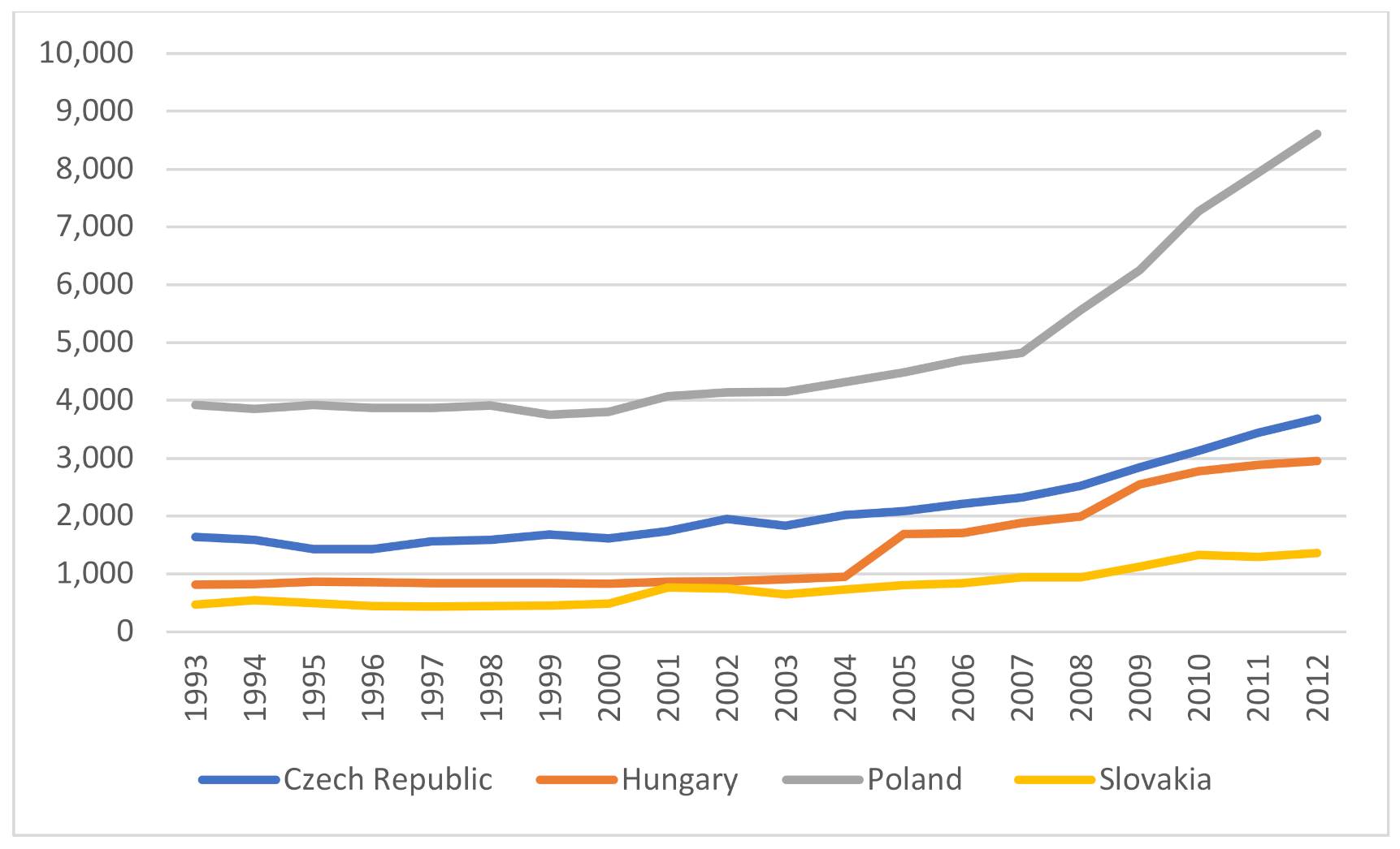
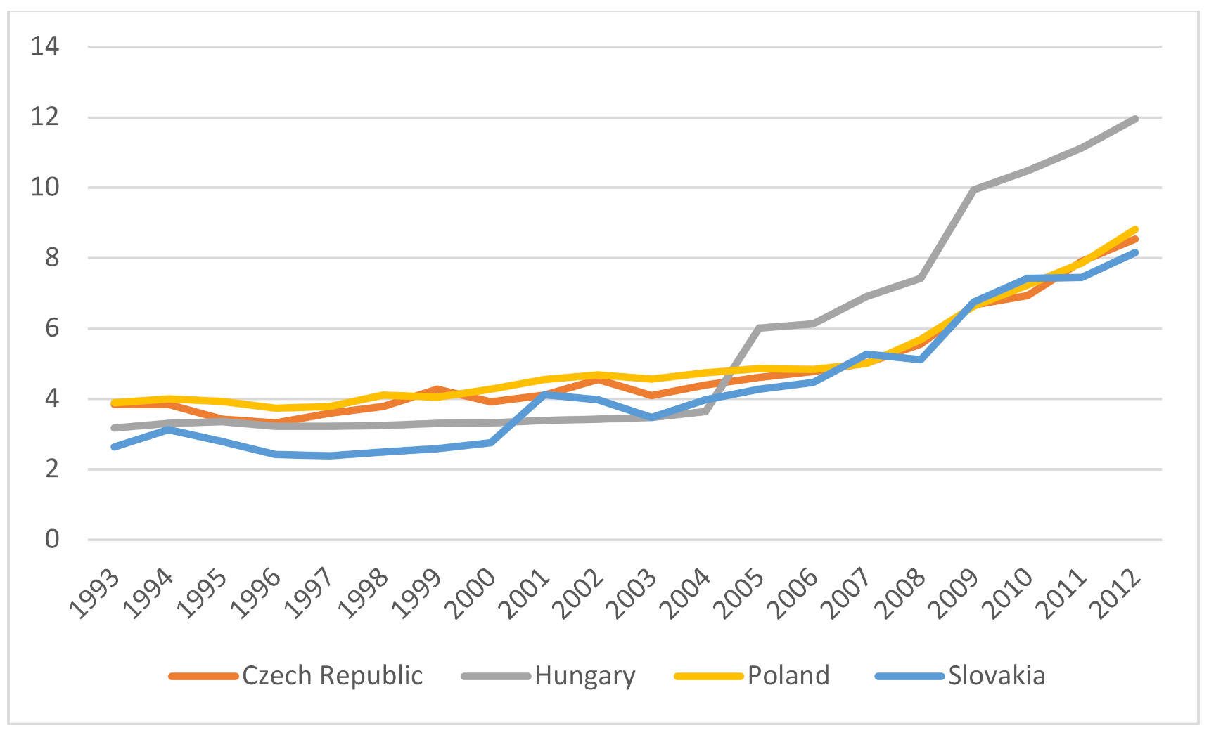
	SUBS	20	1.900	1.553	1.000	6.000

. In the analyzed period 1993–2012, the level of renewable energy production in all countries of the Visegrad Group increased in absolute terms (cf. Figure 1) and renewable energy also increasingly replaced energy from fossil fuels (cf. Figure 2). However, the share of renewable energy in total energy production, although increasing, remained relatively low, 4.3–5.5%, on average. The EPS index also showed an upward trend. On average, the highest level of overall stringency of environmental policy was recorded in Hungary, while, in Poland, the highest average restrictiveness of environmental taxes and emission standards was observed and, in Slovakia, subsidies. The highest average CO₂ emissions per capita in 1993–2012 occurred in the Czech Republic and the lowest in Hungary.

Table 3. Cross-sectional dependency (CD) test for model 1.

Dependent Variable	Breusch–Pagan LM	Pesaran Scaled LM	Bias-Corrected Scaled LM	Pesaran CD
RE_P	27.216 ***	6.125 ***	6.029 ***	−3.620 ***
EPS	27.714 ***	6.268 ***	6.173 ***	−3.343 ***
GDP	15.660 ***	2.788 ***	2.693 ***	−3.596
CDIO	31.986 ***	7.501 ***	7.406 ***	−3.610 ***
GINI	23.408 ***	5.025 ***	4.930 ***	−3.663 ***

*** 0.01 significance level.

,

Table 4. Cross-sectional dependency test (CD) for model 2.

Dependent Variable	Breusch–Pagan LM	Pesaran Scaled LM	Bias-Corrected Scaled LM	Pesaran CD
RE_S	23.408 ***	5.025 ***	4.930 ***	−3.663 ***
EPS	26.251 ***	5.846 ***	5.751 ***	−3.590
GDP	15.396 ***	2.712 ***	2.618 ***	−3.589 ***
CDIO	23.832 ***	5.148 ***	5.053 ***	−3.646
GINI	22.878 ***	4.872 ***	4.777 ***	−3.621 ***

*** 0.01 significance level.

,

Table 5. Cross-sectional dependency test (CD) for model 3.

Dependent Variable	Breusch–Pagan LM	Pesaran Scaled LM	Bias-Corrected Scaled LM	Pesaran CD
RE_P	22.878 ***	4.872 ***	4.777 ***	−3.908 ***
TAX	18.989 ***	3.7496 ***	3.654 ***	−3.612 ***
STAND	24.663 ***	5.388 ***	5.292 ***	−3.682 ***
SUBS	27.798 ***	6.293 ***	6.197 ***	−3.644 ***
GDP	16.341 ***	2.985 ***	2.890 ***	−3.603 ***
CDIO	27.804 ***	6.294 ***	6.199 ***	−3.655 ***
GINI	23.510 ***	5.055 ***	4.959 ***	−3.663 ***

*** 0.01 significance level.

and

Table 6. Cross-sectional dependency test (CD) for model 4.

Dependent Variable	Breusch–Pagan LM	Pesaran Scaled LM	Bias-Corrected Scaled LM	Pesaran CD
RE	31.680 ***	7.413 ***	7.318 ***	−3.902 ***
TAX	32.800 ***	7.736 ***	7.641 ***	−3.895 ***
STAND	23.779 ***	5.132 ***	5.037 ***	−3.686 ***
SUBS	27.871 ***	6.313 ***	6.218 ***	−3.648 ***
GDP	16.001 ***	2.887 ***	2.792 ***	−3.593 ***
CDIO	23.857 ***	5.155 ***	5.060 ***	−3.690 ***
GINI	22.885 ***	4.874 ***	4.779 ***	−3.643 ***

*** 0.01 significance level.

show the test results of cross-sectional dependence (CD) tests. According to the study by Wolde-Rufael and Weldemeskel [33], we used the Breusch–Pagan LM test, Pesaran scaled LM test, bias-corrected scaled LM test and Pesaran CD test. As can be seen from the tables, most CD tests show that cross-sectional dependence is present for each of the panel, but the Pesaran CD test does not show that cross-sectional dependence when GDP (in model 1), EPS and CDIO (in model 2) variables are used as dependent variables. Still, the majority of the CD tests show that there is correlation in the panel. In our analyses, we adopted a significance level of 0.05.

Since the data are cross-sectionally dependent, we applied the second generation of unit root tests. For the EPS, STAND, RE_S, RE_P variables, when a unit root test with no trend is used, we find that it is non-stationary in its level but, when we applied panel unit root tests to the first difference, the variable is I(1). For the rest of the series, they are panel non-stationary in their levels but their first difference was stationary. Robustness check was based on the first-generation of unit root tests which showed that, when we exclude trend, they are I(1) (cf.

Table 7. Second generation of unit root tests.

		MW	MW	CIPS	CIPS	MW	MW	CIPS	CIPS
		Level	Level	Level	Level	Diff	Diff	Diff	Diff
		No Trend	with Trend	No Trend	with Trend	No Trend	with Trend	No Trend	with Trend
Variable	Lags	Statistic	Statistic	Statistic	Statistic	Statistic	Statistic	Statistic	Statistic
EPS	0	24.278	71.933 *	−5.241 ***	−2.820 **	635.576 ***	513.648 ***	−17.290 ***	−15.878 ***
EPS	1	13.684	48.25	−1.940 *	0.744	300.610 ***	228.663 ***	−8.170 ***	−6.394 ***
EPS	2	13.576	32.687	−1.691 *	1.533	138.223 ***	116.281 ***	−3.371 ***	−2.373 ***
EPS	3	18.206	38.855	−1.178	1.73	91.795 ***	61.771	−0.996	−0.253
TAX	0	77.153	93.514 ***	0.193	−0.860	604.747 ***	492.275 ***	−15.550 ***	−13.610 ***
TAX	1	154.278 ***	181.443 ***	0.224	−1.035	402.315 ***	300.299 ***	−11.121 ***	−9.659 ***
TAX	2	43.447	69.219	2.395	2.328	233.845 ***	175.366 ***	−4.627 ***	−2.003 **
TAX	3	84.154 **	136.425 ***	1.648	0.826	289.071 ***	229.607 ***	−2.146 **	1.756
STAND	0	11.678	36.064 *	−6.143 ***	−4.759 ***	545.947 ***	420.751 ***	−16.778 ***	−14.516 ***
STAND	1	9.453	30.476	−5.703 ***	−4.059 ***	237.337 ***	158.799 ***	−10.337 ***	−7.988 ***
STAND	2	10.553	25.197	−5.279 ***	−3.675 ***	122.807 ***	72.707 *	−9.714 ***	−7.812 ***
STAND	3	10.257	33.031	−2.533 **	0.172	78.930 **	40.771	−3.433 ***	−1.05
SUBS	0	186.928 ***	214.022 ***	−6.338 ***	−7.020 ***	1095.143 ***	835.562 ***	−18.636 ***	−17.083 ***
SUBS	1	111.509 ***	116.138 ***	−1.735	−1.618	500.562 ***	449.806 ***	−9.128 ***	−6.763 ***
SUBS	2	100.622 ***	110.253 ***	−0.913	1.082	284.712 ***	234.589 ***	−4.018 ***	−2.446 *
SUBS	3	30.849	38.741	1.962	2.009	199.269 ***	146.978 ***	−0.873	3.201
RE_S	0	31.767	56.13 *	−2.935 **	−4.499	647.016 ***	614.965 ***	−17.646 ***	−16.931 ***
RE_S	1	16.423	33.442	−1.064	−1.833	281.107 ***	263.700 ***	−9.788 ***	−8.196 ***
RE_S	2	14.169	42.476	0.062	−1.527	164.649 ***	139.738 ***	−5.069 ***	−3.042 ***
RE_S	3	12.521	31.889	0.661	−1.235	104.738 ***	111.416 ***	−3.785 ***	−2.057 ***
RE_P	0	17.346	100.394 ***	−4.123 ***	−3.533 ***	775.144 ***	652.657 ***	−17.444 ***	−15.699 ***
RE_P	1	13.035	73.394	−3.796 ***	−2.862 ***	378.619 ***	313.510 ***	−11.171 ***	−8.968 ***
RE_P	2	13.751	62.63	−3.363 ***	−2.391 **	215.706 ***	164.31 ***	−6.078 ***	−3.314 ***
RE_P	3	7.666	61.844	−2.799 **	−2.793 **	151.096 ***	114.875 ***	−4.783 ***	−2.257 **
GDP	0	24.526 ***	18.158 **	−4.646 ***	−3.578 ***	61 ***	38.935 ***	−5.778 ***	−4.1 ***
GDP	1	14.747 *	10.199	−1.652 *	−0.86	40.719 ***	49.844 ***	−1.101	0.435
GDP	2	9.529	2.943	1.689	3.732	41.563 ***	24.51 ***	2.22	3.419
GDP	3	12.204	1.334	4.766	7.43	3.486	1.336	6.593	6.219
CDIO	0	6.75	16.63 **	−1.139	−0.133	92.123 ***	68.269 ***	−6.315 ***	−5.239 ***
CDIO	1	3.322	5.397	−1.143	0.598	45.487 ***	29.706 ***	−4.044 ***	−3.746 ***
CDIO	2	2.03	2.751	−0.339	1.599	16.608 **	8.861	−0.557	0.369
CDIO	3	2.008	3.707	0.063	0.958	14.702 *	6.712	−0.113	0.773
GINI	0	13.051	15.078 **	−0.505	−0.621	83.934 ***	63.659 ***	−4.957 ***	−3.863 ***
GINI	1	13.064	23.156 ***	−1.839 **	−1.46 *	47.024 ***	32.472 ***	−2.798 ***	−1.588 **
GINI	2	9.81	15.01 **	−1.42 *	−0.54	31.958 ***	19.906 ***	−0.51	1.404
GINI	3	5.122	17.246 **	0.953	1.872	28.446 ***	17.034 **	2.221	4.72

*** 0.01 significance level, ** 0.05 significance level and * 0.1 significance level.

).

Since our series are all non-stationary and I(1), according to [33], we applied the Pedroni panel cointegration test, as well as the Kao test. As it can be seen in

Table 8. Panel cointegration tests. Pedroni panel cointegration test and Kao Residual Cointegration for model 1.

Model 1
	No Trend	with Trend
Method	Statistic	Statistic
Panel v-Statistic	−0.503	−0.110
Panel rho-Statistic	0.693	1.186
Panel PP-Statistic	−3.253 ***	−4.399 ***
Panel ADF-Statistic	−2.118 ***	−3.067 ***
Panel rho-Statistic	1.544	2.283
Panel PP-Statistic	−11.136 ***	−12.549 ***
Panel ADF-Statistic	−5.272 ***	−5.716 ***
Test
Modified Dickey–Fuller t	−4.648 ***	3.566 ***
Dickey–Fuller t	−4.240 ***	3.827 ***
Augmented Dickey–Fuller t	−0.967 ***	1.146
Unadjusted modified Dickey–Fuller	−5.465 ***	4.494 ***
Unadjusted Dickey–Fuller t	−4.396 ***	4.041 ***

*** 0.01 significance level.

,

Table 9. Panel cointegration tests. Pedroni panel cointegration test and Kao Residual Cointegration for model 2.

Model 2
	No Trend	with Trend
Method	Statistic	Statistic
Panel v-Statistic	−0.366	−0.265
Panel rho-Statistic	0.747	1.214
Panel PP-Statistic	−3.165 ***	−4.437 ***
Panel ADF-Statistic	−2.2106 ***	−3.064 ***
Panel rho-Statistic	1.603	2.223
Panel PP-Statistic	−9.101 ***	−10.295 ***
Panel ADF-Statistic	−4.221 ***	−5.898 ***
Test
Modified Dickey–Fuller t	−4.403 ***	3.438 ***
Dickey–Fuller t	−4.173 ***	3.836 ***
Augmented Dickey–Fuller t	−1.004	1.227
Unadjusted modified Dickey–Fuller	−5.548 ***	4.559 ***
Unadjusted Dickey–Fuller t	−4.403 ***	4.106 ***

*** 0.01 significance level

,

Table 10. Panel cointegration tests. Pedroni panel cointegration test and Kao Residual Cointegration for model 3.

Model 3
	No Trend	with Trend
Method	Statistic	Statistic
Panel v-Statistic	−0.011	−0.520
Panel rho-Statistic	1.462	2.126
Panel PP-Statistic	−3.989 ***	−4.770 ***
Panel ADF-Statistic	−2.021 ***	−2.259 ***
Panel rho-Statistic	2.381	3.118
Panel PP-Statistic	−10.447 ***	−11.379 ***
Panel ADF-Statistic	−5.652 ***	−6.625 ***
Test
Modified Dickey–Fuller t	1.596 **	2.067 **
Dickey–Fuller t	1.880 **	2.281 ***
Augmented Dickey–Fuller t	1.088	1.491 *
Unadjusted modified Dickey–Fuller	4.181 ***	4.262 ***
Unadjusted Dickey–Fuller t	2.880 ***	3.045 ***

*** 0.01 significance level, ** 0.05 significance level * 0.1 significance level

,

Table 11. Panel cointegration tests. Pedroni panel cointegration test and Kao Residual Cointegration for model 4.

Model 4
	No Trend	with Trend
Method	Statistic	Statistic
Panel v-Statistic	−0.107	−0.689
Panel rho-Statistic	1.483	2.234
Panel PP-Statistic	−3.684 ***	−4.425 ***
Panel ADF-Statistic	−2.093 ***	−3.378 ***
Panel rho-Statistic	2.413	3.159
Panel PP-Statistic	−11.126 ***	−12.502 ***
Panel ADF-Statistic	−5.750 ***	−6.704 ***
Test
Modified Dickey–Fuller t	5.210 ***	4.203 ***
Dickey–Fuller t	4.891 ***	4.321 ***
Augmented Dickey–Fuller t	0.778	1.118
Unadjusted modified Dickey–Fuller	6.844 ***	5.476 ***
Unadjusted Dickey–Fuller t	5.181 ***	4.585 ***

*** 0.01 significance level.

and

Table 12. Hausman tests for model 1.

Equation (1)
MG and PMG	MG and DFE	DFE and PMG
H0: PMG estimator is efficient and consistent but MG is not efficient	H0: DFE estimator is efficient and consistent but MG is not efficient	H0: PMG estimator is efficient and consistent but DFE is not efficient
ρ – value = 1.000	ρ – value = 0.970	ρ – value = 0.999
Since we could not reject the H0, the PMG estimator is selected because it is efficient and consistent.	Since we could not reject the H0, the DFE estimator is selected because it is efficient and consistent.	Since we could not reject the H0, the PMG estimator is selected because it is efficient and consistent.

, both cointegration tests reject the hypothesis of no cointegration. This means that there exists a cointegrating vector among these variables.

In the next step, we ran tests to determine which type of estimator we should use. According to [33], we have to decide between PMG (pooled mean group), MG (mean group) and DFE (dynamic fixed effects) estimators. The results of these tests are presented in Table 12,

Table 13. Hausman tests for model 2.

Equation (2)
MG and PMG	MG and DFE	DFE and PMG
H0: PMG estimator is efficient and consistent but MG is not efficient	H0: DFE estimator is efficient and consistent but MG is not efficient	H0: PMG estimator is efficient and consistent but DFE is not efficient
ρ – value = 0.7820	ρ – value = 0.001	ρ – value = 0.7910
Since we could not reject the H0, the PMG estimator is selected because it is efficient and consistent.	Since we rejected the H0, the MG estimator is selected because it is efficient and consistent.	Since we could not reject the H0, the PMG estimator is selected because it is efficient and consistent.

,

Table 14. Hausman tests for model 3.

Equation (3)
MG and PMG	MG and DFE	DFE and PMG
H0: PMG estimator is efficient and consistent but MG is not efficient	H0: DFE estimator is efficient and consistent but MG is not efficient	H0: PMG estimator is efficient and consistent but DFE is not efficient
ρ – value = 1.0000	ρ – value = 0.000	ρ – value = 0.999
Since we could not reject the H0, the PMG estimator is selected because it is efficient and consistent.	Since we rejected the H0, the MG estimator is selected because it is efficient and consistent.	Since we could not reject the H0, the PMG estimator is selected because it is efficient and consistent.

and

Table 15. Hausman tests for model 4.

Equation (4)
MG and PMG	MG and DFE	DFE and PMG
H0: PMG estimator is efficient and consistent but MG is not efficient	H0: DFE estimator is efficient and consistent but MG is not efficient	H0: PMG estimator is efficient and consistent but DFE is not efficient
ρ – value = 1.000	ρ – value = 1.000	ρ – value = 1.000
Since we could not reject the H0, the PMG estimator is selected because it is efficient and consistent.	Since we could not reject the H0, the DFE estimator is selected because it is efficient and consistent.	Since we could not reject the H0, the PMG estimator is selected because it is efficient and consistent.

.

The Hausman tests did not reject the null hypothesis of homogenous long-run coefficients at the 5% significance level for any of the models. This suggests that PMG is the preferred estimator, when compare with MG. As can be seen in Table 12, Table 13, Table 14 and Table 15, the Hausman tests show that both the DFE and PMG methods are more efficient and consistent than the MG method. Based on the results of these tests, we chose the PMG model (it allows for heterogeneity in the short-run) [33]. The focus of our analysis is on average cross-country elasticities, so we proceeded with the results obtained by using the PMG estimates. The results of the PMG estimates are presented in

Table 16. Long-run and short-run coefficients for model 1.

Dep. var: RE_P	Coefficient
Independent Variables	ARDL (2, 1, 1, 1, 1) Model
A: Long-run
EPS	1.307121 ***
GDP	−0.026203 ***
CDIO	0.575582
GINI	0.892098 ***
B: Panel short-run equation
COINTEQ01	−0.301405 **
D(RE_P(−1))	0.066794
D(EPS)	−0.238699
D(GDP)	−0.000124
D(CDIO)	−0.342775 ***
D(GINI)	0.349815 **
C	0.541036 *
C: Short-term country-specific estimation results	Czech Rep.	Hungary	Poland	Slovakia
COINTEQ01	−0.107913 ***	−0.159204 ***	−0.782121 ***	−0.156384 ***
D(RE_P(−1))	−0.070345	0.457215 ***	−0.14276 ***	0.023067
D(EPS)	−0.059845	−0.118055	−0.747412	−0.029482
D(GDP)	−0.001128 ***	−0.005445 ***	0.001133 ***	0.004946 ***
D(CDIO)	−0.305492 ***	−0.376675 ***	−0.402409 ***	−0.286524
D(GINI)	0.138742 *	0.573628 ***	0.64381 ***	0.043079
C	0.195022 ***	0.269473 ***	1.454022 ***	0.245628 ***

*** 0.01 significance level, ** 0.05 significance level and * 0.1 significance level.

,

Table 17. Long-run and short-run coefficients for model 2.

Dep. var.: RE_S	Coefficient
Independent Variables	ARDL (2, 1, 1, 1, 1) Model
A: Long-run equation
EPS	1.146486 ***
GDP	−0.018767 ***
CDIO	−0.1571
GINI	0.910546 ***
B: Short-run equation
COINTEQ01	−0.317881 **
D(RE_S(−1))	0.061948
D(EPS)	−0.305646
D(GDP)	−0.001262
D(CDIO)	−0.447781 ***
D(GINI)	0.23424 *
C	−0.141487
C: Short-term country-specific estimation results	Czech Rep.	Hungary	Poland	Slovakia
COINTEQ01	−0.082221 ***	−0.147394 ***	−0.771811 ***	−0.270096 ***
D(RE_S(−1))	−0.024316	0.295896 ***	−0.098545 ***	0.074757
D(EPS)	−0.090586	−0.135723	−0.663541	−0.332732
D(GDP)	−0.001506 ***	−0.004674 ***	−0.000977 ***	0.002109 ***
D(CDIO)	−0.672579 ***	−0.409659 ***	−0.35457 ***	−0.354315
D(GINI)	0.062123	0.34259 ***	0.537525 ***	−0.005278
C	−0.006779 ***	−0.058612 ***	−0.43764 ***	−0.063094 ***

*** 0.01 significance level, ** 0.05 significance level and * 0.1 significance level.

,

Table 18. Long-run and short-run coefficients for model 3.

Dep. var.: RE_P	Coefficient
Independent Variables	ARDL (2, 1, 1, 1, 1, 1, 1) Model
A: Long-run equation
TAX	0.164796 *
STAND	0.530384 ***
SUBS	0.58742 ***
GDP	−0.167177
CDIO	−0.028537
GINI	0.448806
B: Short-run equation
COINTEQ01	−0.516378 ***
D(RE_P)	0.087325
TAX	−0.020995
STAND	−0.272442
SUBS	−0.286113
GDP	−0.051947
CDIO	−0.400156 ***
GINI	0.396876 **
C	1.311816 ***
C: Short-term country-specific estimation results	Czech Rep.	Hungary	Poland	Slovakia
COINTEQ01	−0.132193 ***	−0.310492 ***	−0.987936 ***	−0.634891 ***
D(RE_P)	0.020368	0.276326 ***	−0.032515 ***	0.08512 **
TAX	−0.043411	−0.103229	−0.303839	0.366497
STAND	−0.044312	−0.341423	−0.343485	−0.360547
SUBS	−0.1331	−0.447897	−0.426556	−0.136898
GDP	−0.038220 ***	−0.058317 ***	−0.300582 ***	0.189333 ***
CDIO	−0.425234 ***	−0.616221 ***	−0.170466 ***	−0.388706
GINI	0.143155	0.44211 ***	0.941321 ***	0.060918
C	0.36197 ***	0.740631 ***	2.757216 ***	1.387447 ***

*** 0.01 significance level, ** 0.05 significance level and * 0.1 significance level.

and

Table 19. Long-run and short-run coefficients for model 4.

Dep. var.: RE_S	Coefficient
Independent Variables	ARDL (2, 1, 1, 1, 1, 1, 1) Model
A: Long-run equation
TAX	0.07155
STAND	0.390608 ***
SUBS	0.446404 ***
GDP	−0.118605
CDIO	−0.442481 ***
GINI	0.239728 ***
B: Short-run equation
COINTEQ01	−0.588496 ***
D(RE_S(−1))	0.137053 ***
D(TAX)	−0.041921
D(STAND)	−0.249478
D(SUBS)	−0.268462
D(GDP)	−0.062913
D(CDIO)	−0.43018 ***
D(GINI)	0.368194
C	0.306191 ***
Short-term country-specific estimation results	Czech Rep.	Hungary	Poland	Slovakia
COINTEQ01	−0.128592 ***	−0.310628 ***	−0.992579 ***	−0.92182 ***
D(RE_S(−1))	0.065362 **	0.228196 ***	0.023197 ***	0.231458 ***
D(TAX)	0.06853	−0.068924	−0.200671	0.033383
D(STAND)	−0.048682	−0.273052	−0.191584	−0.484594
D(SUBS)	−0.145388	−0.355405	−0.352987	−0.220067
D(GDP)	−0.04299 ***	−0.068797 ***	−0.227885 ***	0.088021 ***
D(CDIO)	−0.805257 ***	−0.55798 ***	−0.116 ***	−0.241515
D(GINI)	0.056986	0.326386 ***	1.0541 ***	0.035192 *
C	0.099942 ***	0.141778 ***	0.515109 ***	0.467935 ***

*** 0.01 significance level, ** 0.05 significance level and * 0.1 significance level.

. As the theory predicted, the error-correction coefficients are significantly negative. Table 16 shows the estimated parameters for model 1. For the long-term relationship, three factors had a statistically significant impact on the volume of renewable energy production (RE_P), namely, the environmental policy stringency (coefficient = 1.307), the GDP per capita growth (coefficient = −0.026) and the Gini index (coefficient = 0.892). CO₂ emissions per capita (CDIO, the negative relationship) turned out to be statistically insignificant. In the short term, the volume of renewable energy production was statistically significantly influenced by the change in CO₂ emissions per capita (coefficient = −0.343) and the change in the Gini index (coefficient = 0.35). The ECM variable coefficient (COINTEQ01) is equal to −0.301. This negative sign indicates a convergent correction mechanism for deviations from the long-term equilibrium in the model.

The analysis of short-term relationships for individual countries shows that, for the Czech Republic, statistically significant variables were the change in GDP per capita growth (coefficient = −0.001) and the change in CO₂ emissions per capita (coefficient = −0.305). The change in the delayed volume of renewable energy produced, the change in the restrictiveness of the environmental policy and the change in the Gini index (at the significance level of 0.05) turned out to be statistically insignificant. For Hungary, the following were statistically significant: change in delayed renewable energy production (coefficient = 0.457), change in GDP per capita growth (coefficient = −0.005), change in CO₂ emissions per capita (coefficient −0.377) and change in the Gini index (coefficient = 0.574). For Poland, the following were statistically significant: change in delayed production of renewable energy (coefficient = −0.143), change in GDP per capita growth (coefficient = 0.001), change in CO₂ emissions per capita (coefficient = −0.402) and change in the Gini index (0.644). For Slovakia, only the change in the GDP per capita growth turned out to be statistically significant (coefficient = 0.005).

Table 17 presents the estimated parameters for model 2. For the long-term dependence, significant determinants of the share of renewable energy production in total energy production were the environmental policy stringency (coefficient = 1.146), the GDP per capita growth (coefficient = −0.019) and the Gini index (coefficient = 0.911). For the short-term relationship, only the change in CO₂ emissions per capita was significant (coefficient = −0.448). The lower part of Table 17 shows the short-term relationships for individual countries. In the case of the Czech Republic, the change in GDP per capita growth (coefficient = −0.002) and the change in CO₂ emissions per capita (coefficient = −0.673) proved to be significant. For Hungary, the following variables were statistically significant: the change in the delayed share of renewable energy in the total energy production (coefficient = 0.3), the change in GDP per capita growth (coefficient = −0.005), the change in CO₂ emissions per capita (coefficient = −0.41) and the change in the Gini index (coefficient = 0.343). Similarly, for Poland, the change of delayed share of renewable energy in total energy production (coefficient = −0.099), the change in GDP per capita growth (coefficient = −0.001), the change of CO₂ emissions per capita (coefficient = −0.355) and change in the Gini index (coefficient = 0.538) proved to be statistically significant. For Slovakia, only the change in GDP per capita growth turned out to be statistically significant (coefficient = 0.002).

Table 18 presents the estimated coefficients for model 3. For the long-term dependence, the significant determinants of the volume of renewable energy production were the stringency of emission standards (coefficient = 0.53) and the stringency of subsidies (coefficient = 0.587). The restrictiveness of environmental taxes had no significant impact on the volume of renewable energy production (at the 0.05 level of significance) in the short nor in the long term. On the other hand, for the short-term relationship, two variables were significant, namely, the change in CO₂ emissions per capita (coefficient = −0.4) and the change in the Gini index (coefficient = 0.397).

In the case of short-term relationships, the change in GPD per capita growth was statistically significant for each country (the coefficients were −0.038, −0.058, −0.301 and 0.189 for the Czech Republic, Hungary, Poland and Slovakia, respectively). The change in the delayed volume of renewable energy production turned out to be statistically significant for Hungary (coefficient = 0.276), Poland (coefficient = −0.0325) and Slovakia (coefficient = 0.085). The change in CO₂ emissions per capita proved to be statistically significant in the case of the Czech Republic (coefficient = −0.425), Hungary (coefficient = −0.616) and Poland (coefficient = −0.17). Only in Hungary and Poland, the Gini index turned out to be statistically significant (the coefficients were 0.442 and 0.941, respectively).

Table 19 presents the estimated parameters for the model 4. In the long run, significant determinants of the share of renewable energy production in total energy production were the stringency of emission standards (coefficient = 0.391) and the stringency of subsidies (coefficient = 0.446), CO₂ emissions per capita (coefficient = −0.442) and the Gini index (coefficient = 0.24). For the short-term relationship, the following were statistically significant: change in delayed share of renewable energy production in total energy production (coefficient = 0.137) and change in CO₂ emissions per capita (coefficient = −0.43).

Regarding short-term relationships for the Czech Republic, the change in the delayed share of renewable energy production in total energy production (coefficient = 0.065), the change in GDP per capita growth (coefficient = −0.043) and the change in CO₂ emissions per capita (coefficient = −0.805) turned out to be statistically significant. For Hungary, the following were statistically significant: the change in the delayed share of renewable energy production in total energy production (coefficient = 0.228), the change in GDP per capita growth (coefficient = 0.069), the change in CO₂ emissions per capita (coefficient = 0.558) and the change in the Gini index (coefficient = 0.326). In the case of Poland, the change in the delayed share of renewable energy production in total energy production (coefficient = 0.023), the change in GDP per capita growth (coefficient = −0.228), the change in CO₂ emissions per capita (coefficient = −0.116) and the change in the Gini index (coefficient = 1.054) proved to be statistically significant. For Slovakia, the following were statistically significant: the change in the delayed share of renewable energy production in total energy production (coefficient = 0.231) and the change in GDP per capita growth (coefficient = 0.088).

For all four models, the convergence speed is close to 57%, which indicates that disequilibrium is corrected within less than two years.

6. Discussion and Conclusions

The instruments of environmental policy used in practice are characterized by heterogeneity and can be classified according to a set of different design features. In this paper, we focus on whether the development of renewable energy can be related to one of these design features, which is policy stringency, given the overall level of stringency and the stringency of individual instruments, i.e., taxes, standards and subsidies. The results of our research study on the Visegrad Group countries indicate that a more stringent environmental policy has a positive impact both on the increase in the absolute volume of renewable energy production, as well as on the replacement of energy from fossil sources. However, we have observed this effect only in the long run, which means that solely consistent and long-term tightening of environmental policies can contribute to promote renewable energy.

Our main findings indicate that renewable energy production is positively influenced not only by the stringency of instruments aimed directly at the development of this energy sector (government subsidies), but also by the stringency of instruments with other environmental goals (emission standards for NOx, SOx, particulate matters and diesel) and by the overall level of restrictiveness of the environmental policy, which includes various types of instruments (intended for renewable energy and others). The impact of subsidies stringency on renewable energy production is only slightly greater than the impact of standards stringency. This result may seem surprising because subsidies aimed directly at supporting renewable energy should have a greater impact on the development of this energy than instruments with other environmental goals (improvement of air quality). In our opinion, only a slightly greater role of subsidies than emission standards in the development of renewable energy results from the fact that the standards are mandatory and failure to meet them results in the necessity to pay high fines or the inability to conduct business activity. Subsidies are voluntary, not all enterprises use them, contrary to the standards that apply to all enterprises. In addition, the weaker impact of subsidies may result from the high level of bureaucracy that is characteristic of post-socialist countries (including the Visegrad Group) and the administrative difficulties associated with obtaining them.

We have not found that strict environmental taxes are a significant determinant of renewable energy generation. Environmental taxes in the Visegrad Group countries are set at a low level and even the increase in their stringency does not result in such an increase in the financial burden on enterprises that would be a significant stimulus to invest in renewable energy sources.

The role of restrictive emission standards and—in general—environmental policy in the development of renewable energy may result from the fact that the tightening of environmental regulations in a given country contributes to these regulations becoming an accepted social norm over time and the level of environmental awareness of the society increases. This, in turn, translates into support for environmentally friendly energy sources.

Similar conclusions about the positive impact of restrictive environmental policy on the development of renewable energy were drawn by the authors, who, however, analyzed only instruments targeting directly renewable energy—feed-in-tariffs [14] and renewable portfolio standards [11,12].

Our research also indicates the influence of other factors on the production of renewable energy, in addition to environmental policy stringency. The relationship between the GDP per capita growth and renewable energy production (measured both in thous. toe and share in total energy supply) is negative and statistically significant in models 1–2. This proves that the economic development of analyzed countries, at least in the long run, decreases the production of renewable energy. The Visegrad Group countries have economies based on fossil fuels and, in our opinion, their economic development, at least in the long term, is strongly correlated with higher combustion of these fuels (higher or more efficient use of existing infrastructure). A negative sign of CO₂ emissions per capita variable is unexpected and statistically significant, in the long run, in model 4 and, in the short run, in all models. The only conclusion we come up with about CO₂ emissions is that, in the Visegrad Group countries, there is probably a time delay in the relation between emissions of CO₂ and production of renewable energy, and its share in total energy production, which was not captured by the models. The Gini index also quite often proves to be statistically significant, which we interpret as a positive impact of accumulation of capital and investors with a sufficiently high level of income in researched countries on the renewable investments.

Our study is not free from limitations. The study only concerns the countries of the Visegrad Group. Moreover, it is confined to the period 1993–2012 (due to data availability). Taking into account the subsequent years, covering the third period of the EU Emissions Trading System, in which the climate policy for enterprises was tightened, could shed new light on the impact of the restrictive nature of environmental policy instruments and CO₂ emissions on the development of renewable energy. We believe that matters regarding the role of environmental policy stringency in boosting cleaner energy deployment need further scientific examinations.

References

1. OECD. Environment at a Glance 2020; OECD Publishing: Paris, France, 2020. [Google Scholar] [CrossRef]
2. Kilinc-Ata, N. The evaluation of renewable energy policies across EU countries and US states: An econometric approach. Energy Sustain. Dev. 2016, 31, 83–90. [Google Scholar] [CrossRef]
3. Marinescu, N. Changes in Renewable Energy Policy and Their Implications: The Case of Romanian Producers. Energies 2020, 13, 6493. [Google Scholar] [CrossRef]
4. Johnstone, N.; Haščič, I.; Popp, D. Renewable Energy Policies and Technological Innovation: Evidence Based on Patent Counts. Environ. Resour. Econ. 2010, 45, 133–155. [Google Scholar] [CrossRef]
5. Bersalli, G.; Menanteau, P.; El-Methni, J. Renewable energy policy effectiveness: A panel data analysis across Europe and Latin America. Renew. Sustain. Energy Rev. 2020, 133, 110351. [Google Scholar] [CrossRef]
6. De Atholia, T.; Flannigan, G.; Lai, S. Renewable Energy Investment in Australia. Bull. Reserve Bank Aust. 2020, 36–46. Available online: https://www.rba.gov.au/publications/bulletin/2020/mar/renewable-energy-investment-in-australia.html (accessed on 21 September 2021).
7. Muhammed, G.; Tekbiyik-Ersoy, N. Development of Renewable Energy in China, USA, and Brazil: A Comparative Study on Renewable Energy Policies. Sustainability 2020, 12, 9136. [Google Scholar] [CrossRef]
8. Menz, F.C.; Vachon, S. The effectiveness of different policy regimes for promoting wind power: Experiences from the states. Energy Policy 2006, 34, 1786–1796. [Google Scholar] [CrossRef]
9. Aguirre, M.; Ibikunle, G. Determinants of renewable energy growth: A global sample analysis. Energy Policy 2014, 69, 374–384. [Google Scholar] [CrossRef] [Green Version]
10. Garcia-Álvarez, M.T.; Cabeza-Garcia, L.; Soares, I. Analysis of the promotion of onshore wind energy in the EU: Feed-in tariff or renewable portfolio standard? Renew. Energy 2017, 111, 256–264. [Google Scholar] [CrossRef]
11. Yin, H.; Powers, N. Do state renewable portfolio standards promote in-state renewable generation? Energy Policy 2010, 38, 1140–1149. [Google Scholar] [CrossRef]
12. Carley, S.; Davies, L.L.; Spence, D.B.; Zirogiannis, N. Empirical evaluation of the stringency and design of renewable portfolio standards. Nat. Energy 2018, 3, 754–763. [Google Scholar] [CrossRef]
13. Haas, R.; Panzer, C.; Resch, G.; Ragwitz, M.; Reece, G.; Held, A. A historical review of promotion strategies for electricity from renewable energy sources in EU countries. Renew. Sustain. Energy Rev. 2011, 15, 1003–1034. [Google Scholar] [CrossRef]
14. Jenner, S.; Groba, F.; Indvik, J. Assessing the strength and effectiveness of renewable electricity feed-in tariffs in European Union countries. Energy Policy 2013, 52, 385–401. [Google Scholar] [CrossRef] [Green Version]
15. Schmidt, T.S.; Sewerin, S. Measuring the temporal dynamics of policy mixes—An empirical analysis of renewable energy policy mixes’ balance and design features in nine countries. Res. Policy 2019, 48, 103557. [Google Scholar] [CrossRef]
16. Polzin, F.; Egli, F.; Steffen, B.; Schmidt, T.S. How do policies mobilize private finance for renewable energy? A systematic review with an investor perspective. Appl. Energy 2019, 236, 1249–1268. [Google Scholar] [CrossRef]
17. OECD. How Stringent are Environmental Policies? Policy Perspectives. 2016. Available online: https://www.oecd.org/environment/how-stringent-are-environmental-policies.htm (accessed on 18 December 2020).
18. Botta, E.; Koźluk, T. Measuring Environmental Policy Stringency in OECD Countries: A Composite Index Approach. OECD Econ. Dep. Work. Pap. 2014, 1177, 1–45. [Google Scholar]
19. Galeotti, M.; Salini, S.; Verdolini, E. Measuring environmental policy stringency: Approaches, validity, and impact on environmental innovation and energy efficiency. Energy Policy 2020, 136, 111052. [Google Scholar] [CrossRef]
20. Sauter, C. How should We Measure Environmental Policy Stringency? A New Approach; IRENE Working Paper 2014. Available online: https://www5.unine.ch/RePEc/ftp/irn/pdfs/WP14-01.pdf (accessed on 20 December 2020).
21. Porter, M.E.; van der Linde, C. Toward a New Conception of the Environment—Competitiveness Relationship. J. Econ. Perspect. 1995, 9, 97–118. [Google Scholar] [CrossRef]
22. Jobert, T.; Karanfil, F.; Tykhonenko, A. Degree Of Stringency Matters: Revisiting The Pollution Haven Hypothesis Based On Heterogeneous Panels And Aggregate Data. Macroecon. Dyn. 2018, 23, 2675–2697. [Google Scholar] [CrossRef]
23. Sadik-Zada, E.R.; Ferrari, M. Environmental Policy Stringency, Technical Progress and Pollution Haven Hypothesis. Sustainability 2020, 12, 3880. [Google Scholar] [CrossRef]
24. Sauvage, J. The Stringency of Environmental Regulations and Trade in Environmental Goods. OECD Trade Environ. Work. Pap. 2014, 3, 1–68. [Google Scholar] [CrossRef]
25. Koźluk, T.; Timiliotis, C. Do environmental policies affect global value chains? A new perspective on the pollution haven hypothesis. OECD Econ. Dep. Work. Pap. 2016, 1282, 1–63. [Google Scholar] [CrossRef]
26. Sung, B.; Song, W.-Y. Does Dynamic Efficiency of Public Policy Promote Export Performance? Evidence from Bioenergy Technology Sector. Energies 2017, 10, 2131. [Google Scholar] [CrossRef] [Green Version]
27. Ahmed, K.; Ahmed, S. A predictive analysis of CO 2 emissions, environmental policy stringency, and economic growth in China. Environ. Sci. Pollut. Res. 2018, 25, 16091–16100. [Google Scholar] [CrossRef] [PubMed]
28. Bigerna, S.; D’Errico, M.; Polinori, P. Heterogeneous impacts of regulatory policy stringency on the EU electricity Industry: A Bayesian shrinkage dynamic analysis. Energy Policy 2020, 142, 111522. [Google Scholar] [CrossRef]
29. Wang, Y.; Sun, X.; Guo, X. Environmental regulation and green productivity growth: Empirical evidence on the Porter Hypothesis from OECD industrial sectors. Energy Policy 2019, 132, 611–619. [Google Scholar] [CrossRef]
30. Albrizio, S.; Koźluk, T.; Zipperer, V. Environmental policies and productivity growth: Evidence across industries and firms. J. Environ. Econ. Manag. 2017, 81, 209–226. [Google Scholar] [CrossRef]
31. Rubashkina, Y.; Galeotti, M.; Verdolini, E. Environmental regulation and competitiveness: Empirical evidence on the Porter Hypothesis from European manufacturing sectors. Energy Policy 2015, 83, 288–300. [Google Scholar] [CrossRef] [Green Version]
32. Johnstone, N.; Haščič, I.; Poirier, J.; Hemar, M.; Michel, C. Environmental policy stringency and technological innovation: Evidence from survey data and patent counts. Appl. Econ. 2012, 44, 2157–2170. [Google Scholar] [CrossRef] [Green Version]
33. Wolde-Rufael, Y.; Weldemeskel, E.M. Environmental policy stringency, renewable energy consumption and CO2 emissions: Panel cointegration analysis for BRIICTS countries. Int. J. Green Energy 2020, 17, 568–582. [Google Scholar] [CrossRef]
34. Wolde-Rufael, Y.; Weldemeskel, E.M. Do environmental taxes and environmental stringency policies reduce CO2 emissions? Evidence from 7 emerging economies. Environ. Sci. Pollut. Res. 2021, 28, 22392–22408. [Google Scholar] [CrossRef]
35. Wang, K.; Yan, M.; Wang, Y.; Chang, C.P. The impact of environmental policy stringency on air quality. Atmos. Environ. 2020, 231, 117522. [Google Scholar] [CrossRef]
36. Khan, Z.; Sisi, Z.; Siqun, Y. Environmental regulations an option: Asymmetry effect of environmental regulations on carbon emissions using non-linear ARDL. Energy Sources Part. A Recover. Util. Environ. Eff. 2019, 41, 137–155. [Google Scholar] [CrossRef]
37. Godawska, J. Environmental policy stringency and its impact on air pollution in Poland. Ekon. I Sr. 2021, 1, 52–67. [Google Scholar] [CrossRef]
38. Ai, H.; Zhou, Z.; Li, K.; Kang, Z.Y. Impacts of the desulfurization price subsidy policy on SO2 reduction: Evidence from China’s coal-fired power plants. Energy Policy 2021, 157, 112477. [Google Scholar] [CrossRef]
39. Dong, Y.; Hou, W.; Xi, L.; Wang, T. Relocate or Innovate? The Impact of Environmental Regulation Stringency on Pollution-Intensive Firms in China (31 March 2020). Available online: http://dx.doi.org/10.2139/ssrn.3586564 (accessed on 18 December 2020).
40. Alexandersson, E. The Effect of Environmental Policies on CO2 Emissions—Using the Environmental Policy Stringency Index. Available online: https://gupea.ub.gu.se/handle/2077/66496 (accessed on 18 December 2020).
41. Menanteau, P.; Finon, D.; Lamy, M.-L. Prices versus quantities: Choosing policies for promoting the development of renewable energy. Energy Policy 2003, 31, 799–812. [Google Scholar] [CrossRef]
42. Dong, C.G. Feed-in tariff vs. renewable portfolio standard: An empirical test of their relative effectiveness in promoting wind capacity development. Energy Policy 2012, 42, 476–485. [Google Scholar] [CrossRef]
43. Alagappan, L.; Orans, R.; Woo, C.K. What drives renewable energy development? Energy Policy 2011, 39, 5099–5104. [Google Scholar] [CrossRef]
44. Shrimali, G.; Kniefel, J. Are government policies effective in promoting deployment of renewable electricity resources? Energy Policy 2011, 39, 4726–4741. [Google Scholar] [CrossRef]
45. Zhao, Y.; Tang, K.K.; Wang, L. Do renewable electricity policies promote renewable electricity generation? Evidence from panel data. Energy Policy 2013, 62, 887–897. [Google Scholar] [CrossRef]
46. Loitera, J.M.; Norberg-Bohm, V. Technology policy and renewable energy: Public roles in the development of new energy technologies. Energy Policy 1999, 27, 85–97. [Google Scholar] [CrossRef]
47. Gawel, E.; Lehmann, P.; Purkus, A.; Söderholm, P.; Witte, K. Rationales for technology-specific RES support and their relevance for German policy. Energy Policy 2017, 102, 16–26. [Google Scholar] [CrossRef]
48. Gostomczyk, W. System aukcyjny jako nowy sposób wspierania OZE. Zesz. Nauk. Szkoły Głównej Gospod. Wiej. W Warszawie 2018, 18, 113–133. [Google Scholar] [CrossRef] [Green Version]
49. Butler, L.; Neuhoff, K. Comparison of feed-in tariff, quota and auction mechanisms to support wind power development. Renew. Energy 2008, 33, 1854–1867. [Google Scholar] [CrossRef] [Green Version]
50. Tanaka, M.; Chen, Y. Market power in renewable portfolio standards. Energy Econ. 2013, 39, 187–196. [Google Scholar] [CrossRef]
51. Brown, T.; Reichenberg, L. Decreasing market value of variable renewables can be avoided by policy action. Energy Econ. 2021, 100, 105354. [Google Scholar] [CrossRef]
52. Bürer, M.J.; Wüstenhagen, R. Which renewable energy policy is a venture capitalist’s best friend? Empirical evidence from a survey of international cleantech investors. Energy Policy 2009, 37, 4997–5006. [Google Scholar] [CrossRef] [Green Version]
53. Pahle, M.; Pachauri, S.; Steinbacher, K. Can the Green Economy deliver it all? Experiences of renewable energy policies with socio-economic objectives. Appl. Energy 2016, 179, 1331–1341. [Google Scholar] [CrossRef] [Green Version]
54. Mu, Y.; Cai, W.; Evans, S.; Wang, C.; Roland-Holst, D. Employment impacts of renewable energy policies in China: A decomposition analysis based on a CGE modeling framework. Appl. Energy 2018, 210, 256–267. [Google Scholar] [CrossRef]
55. Negro, S.O.; Alkemade, F.; Hekkert, M.P. Why does renewable energy diffuse so slowly? A review of innovation system problems. Renew. Sustain. Energy Rev. 2012, 16, 3836–3846. [Google Scholar] [CrossRef] [Green Version]
56. Marques, A.C.; Fuinhas, J.A.; Manso, J.R.P. Motivations driving renewable energy in European countries: A panel data approach. Energy Policy 2010, 38, 6877–6885. [Google Scholar] [CrossRef]
57. Padhan, H.; Padhang, P.C.; Tiwari, A.K.; Ahmed, R.; Hammoudeh, S. Renewable energy consumption and robust globalization(s) in OECD countries: Do oil, carbon emissions and economic activity matter? Energy Strat. Rev. 2020, 32, 100535. [Google Scholar] [CrossRef]
58. Mukhtarov, S.; Humbatova, S.; Hajiyev, N.G.-O.; Aliyev, S. The Financial Development-Renewable Energy Consumption Nexus in the Case of Azerbaijan. Energies 2020, 13, 6265. [Google Scholar] [CrossRef]
59. Sadorsky, P. Renewable energy consumption and income in emerging economies. Energy Policy 2009, 37, 4021–4028. [Google Scholar] [CrossRef]
60. da Silva, P.P.; Cerqueira, P.A.; Ogbe, W. Determinants of renewable energy growth in Sub-Saharan Africa: Evidence from panel ARDL. Energy 2018, 156, 45–54. [Google Scholar] [CrossRef]
61. Gan, J.; Smith, C.T. Drivers for renewable energy: A comparison among OECD countries. Biomass Bioenergy 2011, 35, 4497–4503. [Google Scholar] [CrossRef]
62. Alabi, O.; Ackah, I.; Lartey, A. Re-visiting the renewable energy–economic growth nexus: Empirical evidence from African OPEC countries. Int. J. Energy Sect. Manag. 2017, 11, 387–403. [Google Scholar] [CrossRef] [Green Version]
63. Apergis, N.; Payne, J.E. The causal dynamics between renewable energy, real GDP, emissions and oil prices: Evidence from OECD countries. Appl. Econ. 2014, 46, 4519–4525. [Google Scholar] [CrossRef]
64. Omri, A.; Daly, S.; Nguyen, D.K. A robust analysis of the relationship between renewable energy consumption and its main drivers. Appl. Econ. 2015, 47, 2913–2923. [Google Scholar] [CrossRef]
65. Salim, R.A.; Rafiq, S. Why do some emerging economies proactively accelerate the adoption of renewable energy? Energy Econ. 2012, 34, 1051–1057. [Google Scholar] [CrossRef]
66. Przychodzen, W.; Przychodzen, J. Determinants of renewable energy production in transition economies: A panel data approach. Energy 2020, 191, 116583. [Google Scholar] [CrossRef]
67. Ergun, S.J.; Owusu, P.A.; Rivas, M.F. Determinants of renewable energy consumption in Africa. Environ. Sci. Pollut. Res. 2019, 26, 15390–15405. [Google Scholar] [CrossRef]
68. Akar, B.G. The Determinants Of Renewable Energy Consumption: An Empirical Analysis For The Balkans. Eur. Sci. J. 2016, 12, 594–607. [Google Scholar] [CrossRef]
69. Uzar, U. Is income inequality a driver for renewable energy consumption? J. Clean. Prod. 2020, 255, 120287. [Google Scholar] [CrossRef]
70. Marques, A.C.; Fuinhas, J.A. Drivers promoting renewable energy: A dynamic panel approach. Renew. Sustain. Energy Rev. 2011, 15, 1601–1608. [Google Scholar] [CrossRef]
71. Apergis, N.; Payne, J.E. Renewable energy, output, CO2 emissions, and fossil fuel prices in Central America: Evidence from a nonlinear panel smooth transition vector error correction model. Energy Econ. 2014, 42, 226–232. [Google Scholar] [CrossRef]
72. Bengochea, A.; Faet, O. Renewable energies and CO2 emissions in the European Union. Energy Sources Part B Econ. Plan. Policy 2012, 7, 121–130. [Google Scholar] [CrossRef]
73. Lau, L.S.; Yii, K.J.; Lee, C.Y.; Chong, Y.L.; Lee, E.H. Investigating the determinants of renewable energy consumption in Malaysia: An ARDL approach. Int. J. Bus. Soc. 2018, 19, 886–903. [Google Scholar]
74. Bayar, Y.; Sasmaz, M.U.; Ozkaya, M.H. Impact of Trade and Financial Globalization on Renewable Energy in EU Transition Economies: A Bootstrap Panel Granger Causality Test. Energies 2021, 14, 19. [Google Scholar] [CrossRef]
75. McGee, J.A.; Greiner, P.T. Can Reducing Income Inequality Decouple Economic Growth from CO2 Emissions? Socius Sociol. Res. A Dyn. World 2018, 4, 1–11. [Google Scholar] [CrossRef]
76. Brzeziński, M.; Myck, M.; Najsztub, M. Income Inequality in Transition. New Results for Poland Combining Survey and Tax Return Data. 2020. Available online: https://freepolicybriefs.org/2020/01/13/income-inequality-in-transition-new-results-for-poland-combining-survey-and-tax-return-data/ (accessed on 30 June 2021).
77. Ravallion, M.; Heil, M.; Jalan, J. Carbon Emissions and Income Inequality. Oxf. Econ. Pap. 2000, 52, 651–669. [Google Scholar] [CrossRef]
78. Yang, B.; Ali, M.; Hashmi, S.H.; Shabir, M. Income Inequality and CO2 Emissions in Developing Countries: The Moderating Role of Financial Instability. Sustainability 2020, 12, 6810. [Google Scholar] [CrossRef]
79. McGee, J.A.; Greiner, P.T. Renewable energy injustice: The socio-environmental implications of renewable energy consumption. Energy Res. Soc. Sci. 2019, 56, 101214. [Google Scholar] [CrossRef]
80. Wu, R.; Xie, Z. Identifying the impacts of income inequality on CO2 emissions: Empirical evidences from OECD countries and non-OECD countries. J. Clean. Prod. 2020, 277, 123858. [Google Scholar] [CrossRef]
81. Baek, J.; Gweisah, G. Does income inequality harm the environment?: Empirical evidence from the United States. Energy Policy 2013, 62, 1434–1437. [Google Scholar] [CrossRef]
82. Liu, Q.; Wang, S.; Zhang, W.; Li, J.; Kong, Y. Examining the effects of income inequality on CO2 emissions: Evidence from non-spatial and spatial perspectives. Appl. Energy 2019, 236, 163–171. [Google Scholar] [CrossRef]
83. Kasuga, H.; Takaya, M. Does inequality affect environmental quality? Evidence from major Japanese cities. J. Clean. Prod. 2017, 142, 3689–3701. [Google Scholar] [CrossRef]
84. Aksoy, T. Structural reforms and growth in developing countries. J. Econ. Policy Reform 2019, 22, 325–350. [Google Scholar] [CrossRef]
85. Lv, Z.; Xu, T. Is economic globalization good or bad for the environmental quality? New evidence from dynamic heterogeneous panel models. Technol. Forecast. Soc. Chang. 2018, 137, 340–343. [Google Scholar] [CrossRef]
86. Pedroni, P. Critical Values for Cointegration Tests in Heterogeneous Panels with Multiple Regressors. Oxf. Bull. Econ. Stat. 1999, 61, 653–670. [Google Scholar] [CrossRef]
87. Kao, C. Spurious regression and residual-based tests for cointegration in panel data. J. Econ. 1999, 90, 1–44. [Google Scholar] [CrossRef]
88. Hausman, J.A. Specification tests in econometrics. Econometrica 1978, 46, 1251–1271. [Google Scholar] [CrossRef] [Green Version]
Figure 1. Production of renewable energy (in thousand tons of oil equivalent).
Energies 14 06225 g001
Figure 2. Share of renewable energy production in total energy production (in %).
Energies 14 06225 g002