Abstract
Due to the substantial amounts of money involved and the complex interactions of a number of different factors, managers of oil and gas companies are faced with significant challenges when making investment decisions that will increase business efficiency and achieve competitive advantages, especially through cost control. Due to the various uncertainties of the current period, optimal investment strategies are difficult to determine. Thus, through an economic analysis that includes data analysis, quantitative risk analysis scenarios, modelling and simulations, a work framework, in the form of a generic algorithm, is proposed with the aim of generating a complex procedure for optimizing investment decisions in oil field development. A complex set of elements is considered in the analysis: costs (operational expenditures (OPEX) and capital expenditures (CAPEX), daily drilling rig costs), prices (oil, gas, separation and water injection preparation), production profiles, different types of taxes and discount factors. Above all, oil price volatility plays an essential role and creates uncertainty in relation to profitability and the strategic investment decisions made by oil exploration and production companies.
1. Introduction
As with any scientific paper, it is necessary to demonstrate, on the one hand, the opportunity presented by the study, and, on the other, its topicality and relevance.
Regarding the research opportunity, it should be said that, according to the Fortune Global 500 ranking of the largest companies in terms of revenue for 2020, four of the top 10 corporations operate in the oil industry, while two other companies in the top 10 operate in the energy sphere as their major field and in the oil sector, subsidiarily []. These facts demonstrate the importance and the significance of the contributions made by the petroleum sector to the world economy, such that any study or research concerned with investment decisions in this sector, given the amounts of money considered and circulated, ought to be seen as important.
At the same time, the topicality and relevance of the research is given, on the one hand, by its including and reporting on some of the newest and most important research in the field (over 85% of the titles included in the references section being studies conducted in the last 5 years), and, on the other, the approach proposed in the study, which shows the specific features of the oil and gas industry in relation to a concept not necessarily new, but which has been used extensively in recent years. This is the VUCA approach []. All four components: volatility, uncertainty, complexity and ambiguity, are present in the petroleum industry on a much larger scale than the other important domains. It must be stated from the beginning that the amounts of money invested in the oil industry represent hundreds of millions, even billions of dollars every year.
Therefore, investment decisions are not easy to make and require complex, comprehensive studies that take into account the volatility of the price of crude oil and specific financial issues (which will be described later), as well as various uncertainties about the future of conventional/nonrenewable energy resources, the complexity of the process of transforming crude oil into gasoline and diesel, the ambiguities generated by possible misinterpretations of a range of data and conditions regarding the exploitation of hydrocarbon deposits from one oil field to another [,].
Companies from the oil industry have to be willing and able to perform extensive risk analyses [,]. In this context, it is necessary to resort to economic evaluations that can provide useful information to drive their investment decisions. This approach gives corporate managers the opportunity to decide in a reasoned manner how to prioritize projects and how to make efficient allocations of funds [].
The oil industry is capital-intensive consuming. This is demonstrated by the need to invest in new technologies and equipment, to explore new markets or propose projects in oil field development. These capital investments, so necessary for the development of corporations, are based on risk analyses performed in order to verify the financing capacity of projects. Most projects in the oil industry are evaluated on several levels of risks: economic risk, technical risk, environmental risk, political risk, etc. [].
This paper analyses the major risks related to projects aimed at oil field development. Given the large capital investments required for oil industry projects, economic risk focuses on monetary returns, operating costs (which in many cases are very high), capital costs and other potential factors that influence the price of crude oil.
Related to all the types of risk mentioned above, this paper proposes a risk management framework to help companies make accurate and data-driven decisions when it comes to making investments in oil field development.
For this framework, the authors used, firstly, modelling as a tool (using real data sets). Then, quantitative risk assessments were used, taking into account the concept of the value of money over time (the analysis was performed over a period of 12 years), by discounting cash flows and highlighting the influence of different categories of risks on revenues. In order to complete the scheme for generating the risk management framework, scenario planning was used. This concept envisages exploring various scenarios that could have an impact on cash flow.
To return to the paper’s subject and objectives, it has to be said, related to the VUCA approach, that is critical to anticipating the future and providing guidance to the petroleum companies, by offering well-founded decisions, with modern solutions, in order to bring efficiency in their business activities.
In the current worldwide context of the oil industry, with a fluctuating oil price (information will be presented later within the main body of the paper), and with pressure coming from entities that are encouraging the use of renewable resources and promoting sustainable development, the evaluation of the economic performance of a hydrocarbon field development must be more and more complex, accounting for risks and uncertainties related to the economic environment in which oil companies must operate.
In the light of addressing this problem and finding a pertinent solution, the authors proposed a comprehensive framework as a work methodology (including an economic model) and designed and constructed a workflow that integrates the activity of at least three departments from an oil and gas operator: Reservoir Studies, Field Development and Economics, and which represents the core part of the framework. The workflow, named Integrated Workflow between Petroleum Engineering and Petroleum Economics (shortened to Integrated Workflow) consists of a simulation model whose output data are sent to a probabilistic economic model based on the Discounted Cash Flow method.
Integrated Workflow (acting as a generic algorithm) is an innovative product that is allowing the integration and quantification of risks and uncertainties specific to hydrocarbon field development. It is also a useful tool that is helping the end user to explore and understand the impact of different assumptions on forecast variables, and is providing directions for decisions relating to the need to explore different field development solutions. The workflow was tested using modified data and proved to be flexible, versatile, easy to use and reliable.
2. Literature Review
For any risk type and quantification of uncertainty, the management of risk is requiring the utilization of different techniques, technologies and, in most cases, dedicated tools. These are specific and must be tailored to the particularities of every situation. In relation to the oil and gas industry, the solutions, techniques and tools permits the identification and analysis of risks, but also an assessment of the impact of different variables when evaluating CAPEX and OPEX, in order to set budgets in the downstream and upstream areas. The present paper considers the upstream sector, since it is analysing and modelling the economic performance of an oil field. The large number of risk factors and uncertainties that characterize the oil and gas industry oblige decision makers to build models and tools that integrate the whole set of variables that define the systems operating in the upstream, midstream and downstream areas.
Technical-economic optimization in the performance of an oil field depends on a multitude of parameters being included in the models generated. From this point of view, current articles and updated researches (from the last four to five years), pertaining to the oil and gas industry, will be referred to the throughout the paper. These scientific works concerned subjects relating to the optimization of the decision-making process regarding the improvement of the companies’ profitability.
For specialists in the oil and gas industry, it is necessary to find ways to develop tools for predicting production performance and analyzing the profitability of oil fields []. Nowadays there is a concern to analyze the decline curve (in fact, the DCA method) on a computerized statistical basis with the purpose of making an objective interpretation of the opportunities offered by an oil field [,]. One of the most frequently used methods for estimating the final recovery factor (actually, estimated ultimate recovery—EUR) but also for determining the field performance refers to the Arps DCA variant [].
At the same time, through the decline curve analysis, various models were also built for shale gas reservoirs []. In addition, based on the estimation of the maximum value for the Net Present Value (NPV), an optimal well spacing can be established for an oil field after the comprehensive analysis of many parameters defining the oil field []. On the other hand, the technical-economic optimization must consider predicting production-system behaviour dynamics based on the modelling of the physical characteristics defining the shale-gas reservoir [].
There are various approaches for analysing production performance in the oil and gas industry using the assisted history matching [AHM] technique to generate multiple history matching solutions []. Also, similar in its design to the method proposed in the present paper, an AHM workflow integrates a wide range of uncertainties to predict the response parameters using different tools and concepts: Neural network, Markov Chain Monte Carlo algorithm or reservoir simulator [].
There are studies based on large volumes of data that include field data, laboratory measurements, real time field monitoring, etc., which propose workflows useful in the development of oil fields and that will be able to be used in future developments in the field []. There is also extensive research analysing how various parameters (i.e., crude oil price or oil trade volumes) affect the profitability of oil and gas companies []. In the last four to five years, complex analyses have been published that have considered especially the impact of the changes regarding oil prices on the stock returns of oil and gas companies [,,].
On the other hand, there are different studies and bodies of research that estimate a risk index and propose ways to mitigate the negative impact and economic losses of oil infrastructures (due to hard drilling and production operations conditions, including sand and dust) in order to improve company profitability [,].
It is important to mention that there is a change of terms and meanings related to the transition from intensive use of fossil resources to investments in renewable energy sources, as a transition risk, and which will lead to major changes in oil prices while the need for the quantification of risks in the use of classical resources is mandatory for the creation of sustainable investment strategies, even in the case of the oil and gas industry [,].
The aspects analyzed in this paper consider the quantification of risks and the analysis of the return on investments in the oil and gas industry. In the case of this industry, risk quantification can also be done based on the value at risk (VaR) [,,].
Through the value at risk the probability of the net present value (NPV) exceeding a certain threshold value can be estimated in relation to the influence of risk factors on the NPV’s values []. Also, the performance of the value at risk measure is studied under different distributional models []. In terms of comparing standard risk measures, there are researches that emphasize the superiority of Expected Shortfall against value at risk [].
On the other hand, in many cases two issues are involved in the overall economic risk assessment of a project, namely, NPV, as a method for the economic feasibility, and the Monte Carlo Simulation, as a stochastic approach []. Other approaches also incorporate into the value at risk forecast additional models (such as Markov-Multifractal Switching, MSM) which can support the modelling and forecasting of oil price volatility as well [,].
At the same time, there are studies that consider some threshold methods proposing an integration of the POT (peaks over threshold) concept and which recommend the use of models for forecasting one-day-ahead value at risk [].
Another aspect of forecasting considered to be vital in this article is the influence of crude oil prices in generating the best possible financial results for oil companies. From this point of view, there are various approaches that might be taken. A first example considers a relatively small number of prices in order to analyze the evolution of return and volatility [] (though this is not treated of in this paper, which is concerned with an extended range and large limits). Other authors consider forecasting the volatility of crude oil prices as a critical issue for researchers, market participants and policymakers [].
Since the oil companies look for technical solutions to improve the amount of oil recovered from an oil reservoir, one way is to use one of the methods of Enhanced Oil Recovery (EOR). These methods are costly but can generate significant revenues. Therefore, a field’s hydrocarbon recovery factor is mainly a function of the locations of wells and the reservoir’s condition, including its static properties (porosity, permeability, NTG ratio), dynamic properties (saturations and pressure 3D distributions) and rock-fluid interaction properties (relative permeability and capillary pressures) []. The main role of the well placement process is to establish the best well locations so as to generate the highest profits from hydrocarbon production [] when field development constraints have been taken into account [].
Integrated management of the oil companies is associated with complex decisions that include the dynamics of the new drilling operation and surface facilities, on the one hand, and well/field performance (production and injection rates), on the other. All of these factors have an important impact on field profitability [].
A novel industrial approach refers to dynamic risk analysis (DRA). This new concept intends to create means to monitor changes in operational conditions and to quantify their effect on risk. For the integrated operations related to the oil and gas systems a DRA method called the risk barometer was developed [].
For the analysis of overall risk level variation, it proposes the use of dynamic risk assessment techniques and aggregation methodologies that integrate risk analysis for risk-based decision making for integrated oil and gas operations [].
At the same time, oil companies have to find time-bound solutions to optimize their investments decisions, considering the risks and uncertainties, by which each oil company is able to maximize its profit [,].
3. Data and Methodology
To manage risks and uncertainties and include each risk type and uncertain factor in any activity for an optimum decision it is mandatory to use adequate methods and design suitable methodologies.
The problem analyzed in this case is recognized by oil and gas companies and concerns the possibility of identifying suitable means to provide viable solutions that improve the profitability of companies by using appropriate methodologies in the comparative study of complex technical and economic scenarios. In addition, an approach is introduced that combines theoretical elements of academic analysis with practical aspects, taken from the industry. The discussion is also related to the fact that there are no specific methodologies or procedures explained in sufficient detail to propose complex models or approaches, which consider as many variables and as many forecast parameters as possible, and which can be used by experts from the company in optimizing decisions related to the design of efficient development strategies.
The simulation model discussed in this paper uses the output data to be sent to a probabilistic economic model based on the Discounted Cash Flow method.
This economic model has seventy-eight assumptions relating to the quantification of risks and uncertainties associated with economic or operational environments: oil price, daily rig cost, total drilling days (with modeled risks related to delays and rig problems quantified as drilling days), conditions that are imposing the installation of an artificial lift system (electro submersible pumps—ESP), variations of a well’s flow rate within defined limits, and the possibility of losing the well in the course of an operation due to failure. The twelve forecast variables are focused mainly on economic performance indicators: cumulative discounted cash flow (CDCF), payout time, the profit–investment ratio, CAPEX, OPEX and different types of taxes (profit tax, royalty, ad-valorem tax, etc.).
The economic model [] was constructed in Microsoft Excel and uses a worldwide industry reference software, Oracle Crystal Ball, for the probabilistic calculations (Monte Carlo or Latin Hypercube). The model is very flexible, easy to use and can be modified to adapt it to different hydrocarbon field development solutions. The analysis of the results is performed through percentile and Spearman’s rank correlations [].
In case some of the assumptions defined large intervals, the authors, as part of the workflow, developed a module that subdivides large intervals into smaller subintervals. For example, there might be an assumption that oil price will vary from 20 to 80 USD/stbo (for the last six years). This is quite a large range and, for a more detailed analysis, this wide interval can be subdivided into several non-overlapping smaller intervals. The economic model, as it is designed now, has four assumptions and three subintervals. The number of combinations is N = subintervalsvariables. Changing the assumptions and/or modifying the subintervals is designed to be an easy task and can be performed by virtually anyone. This module generates all the possible combinations of assumptions and subintervals as a new set of cases that are executed sequentially in Oracle Crystal Ball. Upon execution of each of the cases, it generates the report of the run. At the end of the last run, the P50 values are read for all defined forecast variables. The whole operation is controlled by a VBA application integrated into an Excel workbook. This method helps the user to better understand the profitability of the case and to decide which combinations should be considered and which should be discarded. It also gives indications as to whether the field development solution should be revised or optimized to maximize the profit.
Another useful approach is based on Sensitivity analysis principles, which allows the identification of a set of parameters that have the greatest influence in terms of model outputs. In this case, the model outputs are the economic performance indicators:
- -
- POT (Payout Time);
- -
- IRR (Internal Rate of Return)
- -
- PI (Profit–Investment Ratio);
- -
- CNCF (Cumulated Net Cash Flow);
- -
- TT (Total Taxes);
- -
- PT (Profit Tax);
- -
- NPY (Number of Profitable Years).
There are other useful data related to the research. These are:
- -
- The scenario of field development is based on a real oil field in secondary recovery (water injection), located in the northern part of the Arabian Peninsula;
- -
- The considered uncertainties and risks are:
- -
- Drilling time;
- -
- Delays related to problems while drilling;
- -
- Rigs and supply, with potential for the failure of materials;
- -
- Problems and failures related to artificial lift systems (ESP), which might be as serious as losing the well;
- -
- Costs (OPEX, CAPEX and daily drilling rig costs);
- -
- Prices (sales prices for oil and gas, cost of liquid separation and water injection treatment);
- -
- Production profiles;
- -
- The discount factor.
- -
- The model will provide, on one hand, the economic performance parameters as a range and, on the other, the main influencing input parameters.
The designed model considers all the information mentioned above and the outputs help the user to reach decisions for the short-, medium- and long-term evolution of the company and its profitability.
Nowadays we are facing an exponential increase in computational power, which is opening new horizons in the domains of numerical simulation of oil and gas reservoirs and allowing the construction of more and more complex Discounted Cash Flow economic models based on Monte Carlo probabilistic calculation algorithms. The number of parameters defined as distributions of frequencies (called assumptions) and the forecast variables used to model the risks and uncertainties of an economic model can be increased to a level that can incorporate a very large amount of detail.
Through uncertainty quantification and computer simulation, this complex model will be analysed using adequate tools. An economic model is already built in MS Excel using Oracle Crystal Ball (as the industry standard probabilistic engine) []. This economic model is based on the well-known Discounted Cash Flow method and has a high degree of complexity. The whole model, developed by the same authors, is detailed and available for access []. The authors deliberately avoided including in this paper full descriptions and details of the economic model that is used (due to the large volume of information and the need to avoid overlapping paragraphs that will increase the similarity percentage between the two papers).
The starting point in developing the present approach is related to a complex model especially designed to assess the economic performance of an oil field. This model contains 78 input variables (assumptions) and 12 forecast parameters, running 10,000 Monte Carlo trials, in approximately 400 s []. The findings generate a competitive economic model that can help oil and gas companies to determine one of the best development solutions for their investment strategy. This is possible because the model can be considered as a basic scenario which could be integrated with other parameters taking different values.
Currently, the main challenge in this context is finding continuous solutions to improve company profitability by using a comprehensive probabilistic approach. This complex study proposes a comparative analysis by considering different scenarios based on sensitivity analysis. The management focus is to organise an effective decision-making process that will create perspectives for economic benefit and which is adaptable and flexible with respect to investment strategies.
The scope of this article is to present the result of a complex research study performed by the authors, with emphasis on:
- -
- Designing a risk management framework;
- -
- A description of an oil field development solution through an economic analysis;
- -
- Development of a functional Monte Carlo probabilistic economic model using the industry reference software Oracle Crystal Ball;
- -
- Assessing the impact of significant limits on the assumptions and methods so as to overcome potential negative impacts;
- -
- Workflow (a generic algorithm) to integrate Petroleum Engineering with Economics.
3.1. Reservoir Description (Technical Features)
The RAA4 oil field, located in the northern part of the Arabian Peninsula, is a clastic reservoir, and is comprised of five geographical segments separated by communicating faults. These segments have been named Zones 1 to 5. Vertically, it is delineated in five oil bearing formations (Sand 1 to Sand 5), from top to bottom. Sand 1 and Sand 4 are more channeled, the rest more heterogeneous. Four rock types were identified, from lower quality to higher quality, as follows: shale, shale sand, fine sand and coarse sand.
On average, around 85% of the rocks potentially bear hydrocarbons, 33% of the rocks are lower quality rocks with permeability less than 100 mD and 16% of the rocks are shales with less than 4% porosity. The main challenges facing the operating company developing this field are the absence of an active aquifer and the bubble pressure, which is relatively high, varying from 1500 to 2300 psia. The development solutions consider a green field instead of field rehabilitation.
The simulation model was initialized as a black oil system with an original oil-in-place (STOOIP) estimate of 64.8 MMstbo and an original mobile oil-in-place (mobile STOOIP) of 45.1 MMstbo.
The reservoir, generically called RAA4, is treated as a green field and will be developed with 29 oil producers and 18 water injectors. All the wells are vertical and are targeting all the good horizons. The development solution considered:
- -
- That the field oil rate target should be at least 6500 stbo/d and reached in a maximum two years;
- -
- The well economic’s limits, which are: oil rate15 stbo/d, maximum water cut 98% and maximum GOR (gas oil ratio) 2 Mscf/stbo. Once any of the limits are reached, the well is to be shut-in;
- -
- The oil-producing wells are drilled in order to reach and maintain the field oil target;
- -
- Each of the water injection wells are to be assigned a certain number of oil producers and drilled once one of the assigned producers starts;
- -
- The scope of water injectors is to increase the sweep efficiency and maintain the average field pressure close to the initial reservoir pressure;
- -
- The injected water and reservoir fluids volumes are to be balanced to avoid under- or over-pressurization of the field.
The prediction starts at 1st of January 2022 and ends at 1st of April 2034, but all the economic evaluations are to be completed by 1st of January 2034.
Figure 1 shows the initial distribution of oil saturation in the field, as well as the oil producers and the architecture of the water injection wells.
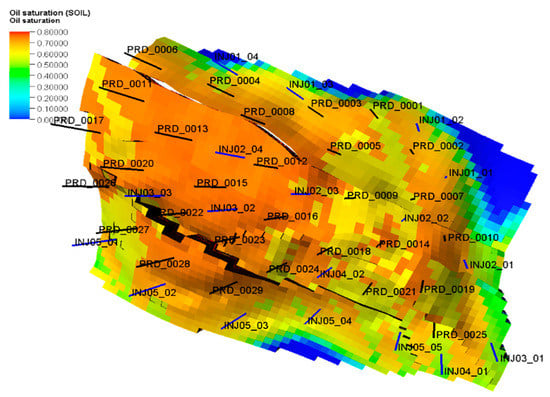
Figure 1.
The RAA4 field and distribution of wells.
The injector–producer ratio is 1:1.6; or, in other words, two injectors to three producers. As good practice, the ratio is 1:2 to 1:4. As can be seen in Figure 1, the injectors are coloured in blue and producers in black. The reasons for the high ration of this FDP proposed solution are: (i) the fault blocks (although in communication, there is a degree of isolation of the separating faults and the channelling system) and (ii) the fast depletion, with the risk of forming a secondary gas cap.
To avoid over-pressurizing the field or the appearance of secondary gas cap—the bubble pressure varies from 1500 to 2300 psia—the VRR (Voidage Replacement Ratio) is set to values in the range 0.95 to 1.1.
Figure 2 presents the field performance.
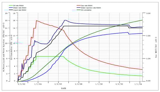
Figure 2.
RAA4 Field Performance.
Under the current development solution, the field attains and maintains a plateau of 6500 stbo/d for almost three years. At the end of the twelve-year forecast, the field will have produced 16 MMstbo, which corresponds to a recovery factor of 24.5%. The total water produced is 36.2 MMstb and the total injected water is 56.6 MMstb. As can be observed, a supplementary source of water is required. The water produced will never be sufficient. Half of the needed injection rate will be available from the produced water after 4.5 years. It must be recalled that all the produced water is from the injected water. The aquifer is too weak to be considered as bringing energy into the system.
Figure 3 shows the number of wells to be released annually.
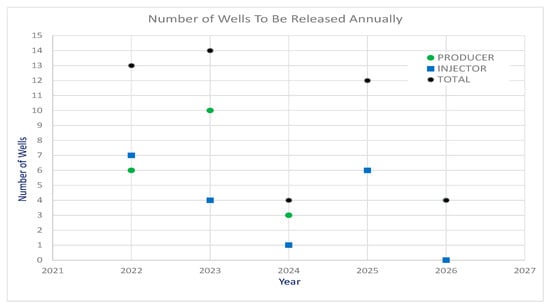
Figure 3.
Number of wells to be released annually.
Analysing Figure 3, it can be observed that the whole drilling program spans the first five years, and it is aggressive in the first year (13 wells to be drilled and commissioned) and in the second year as well (14 wells to be drilled and commissioned). The third and fifth year require only four wells, while the fourth year requires an aggressive well-drilling and commissioning campaign (12 wells).
3.2. Economic Model
The authors developed a probabilistic economic model based on the Discounted Cash Flow method and adapted it to address some of the identified risks related to drilling, production of wells and interventions in their operation, and uncertainties related to selling prices, yearly price escalations, the various costs and other parameters that will be detailed further.
The authors opted to develop an economic model [] complex enough to reflect in relatively high detail the risks and uncertainties, while at the same time keeping the runtime within a reasonable timeframe. As was mentioned above, all the details of the economic model are available []. The following aspects are intended to be highlighted:
- -
- All economic models depend on taxation systems which can vary greatly from country to country. This model is a generic one, considering a simplified tax system from a European country;
- -
- Costs and prices should be considered as indicative and they have been realistically chosen and should be treated as examples;
- -
- The distributions selected for assumptions along with their definitions were decided on the basis of the authors’ experience and they should be treated as examples too. The model is flexible enough to allow the user to change them;
- -
- The CAPEX and OPEX can be much further detailed. They are case specific and must be adapted.
3.3. Integrated Workflow
The authors developed a workflow (generic algorithm) that consists of a complete and customizable innovative solution connecting the domains of Petroleum Engineering and Petroleum Economics. This approach is illustrated in Figure 4.
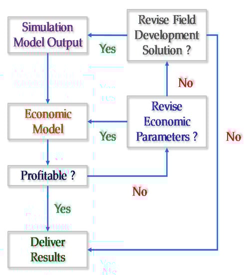
Figure 4.
Integrated workflow.
Simulation Model Output
The simulation model represents the field development solution that the customer will evaluate from a business point of view. The output data are the monthly cumulative of oil, water, gas and water/gas injection.
Economic Model
The economic model is a comprehensive model to assess the business performance of an oil/gas field under development. This model was designed by the authors to be easy to use, easily modified and easily debugged. The data source for production profiles can be either output from a simulation model or from other sources (Decline Curve Analysis— DCA; or Material Balance calculations—MB).
Additionally, the model was designed and implemented in Microsoft Excel using the probabilistic engine Oracle Crystal Ball []. The outputs are the economic performance indicators (Payout Time, Number of Years of Healthy Business, Discounted Cash Flow, Taxes, Profit–Investment Ratio, etc.).
Profitable?
If the business performance indicators are considered good enough, then the outcomes of the study are delivered to the beneficiary.
Revise Economic Parameters
In the case that the business performance parameters are not good enough, there is an option to revise the input parameters (assumptions). The authors have written a script that automatically generates sub-cases of the main case to identify the impact of large ranges for distributions of identified assumptions.
For assumptions that have wide definition ranges and are significantly impacting the business performance indicators, the ranges will be subdivided into narrower intervals. In this case, four parameters were identified and their ranges were subdivided into three subintervals.
The script creates all 34 (81) possible combinations as sub-models, runs all the sub-models and extracts the P50 values for the twelve forecasts (business performance indicators). p-values are widely utilized and implemented in all industry-standard probabilistic software and/or plug-ins like Crystal Ball, @Risk, etc. The script can be easily modified to accommodate more assumptions and more subintervals. Finally, the user can filter out the non-profitable cases.
Revise Field Development Solution?
The user has the option to revise the field development solution and restart the whole process.
As an example, the workflow is applicable as follows: the Subsurface or Reservoir Study team is proposing a field development plan (FDP) for a field representing the input for the Planning team. The Strategic Planning team is responsible for evaluating the economic performance (profitability) of the proposed FDP. In many cases, some technically sound FDPs may be discarded because they are not profitable or not profitable enough. This workflow, as it is developed, is helping the Reservoir Study team to propose, both technically and economically, profitable FDPs. It also connects professionals from different departments who are apparently not related (oil and gas professionals and economists), helping them to work jointly for the company’s success.
4. Results and Discussions
The authors decided to present the results in the same format used in the paper [] cited as the starting point for the current analysis. In fact, it is much easier to understand and follow the two targeted articles.
The following table presents the assumptions and the forecast variables. For practical reasons, some of the forecast variables are embedded in Table 1.

Table 1.
Table with Input Variables and Associated Distribution Settings.
The following points will explain some of the contents of Table 1:
- -
- Start date and End date represent the time interval corresponding to the hydrocarbon production forecast;
- -
- WCT triggering ESPs represents the minimum value of the forecast water cut in a well that is triggering the installation of an ESP (electro-submersible pump—the artificial lift system);
- -
- Equipment’s price inflation represents a coefficient estimating the yearly price increase for any drilling and completion materials;
- -
- Field Cost is an estimated monthly cost to operate the field. It includes all the cash costs (salaries, utilities, etc.) and some of production-related costs. The costs for water injection and fluid separation, separately and together with field cost, go into the Operating Cost (OPEX). This cost itself can be subject to sensitivity analysis;
- -
- Yearly prices increase refers to the yearly increase of selling prices (for oil and gas) and costs (liquid separation, water injection treatment and OPEX);
- -
- Drilling time and Drilling rig cost are two input variables (assumptions) that concern drilling-related costs. Drilling time is converted into money. The variables can be subject to sensitivity analysis;
- -
- Drilling delays related to Risks considers delays from the average drilling time due to some known drilling-associated risks expressed in time and converted into money;
- -
- Well cost is the final cost of a drilled well ready to start producing or injecting;
- -
- Well depreciation time is the time that is required for a well to recover the money spent on its production/injection;
- -
- Rates uncertainty models the associated risks in obtaining field production and takes into account subsurface uncertainties. All the rates (oil, water, liquid, gas and water injection) are simultaneously adjusted with this variable;
- -
- ESP installation frequency models two risk situations: (1) periodic replacement of the ESP due to some pump failures or end of service for ESP, and (2) the risk of losing the well after an ESP intervention;
- -
- Taxes refers to all taxes more complex than a single value. In this paper they are considered as a single value—that is, they are not subject to uncertainty analysis. The taxes are country specific, they may have complex calculation algorithms and can be modelled in various ways and with different degrees of detail;
- -
- Surface facility (CAPEX) embeds the total investments of all surface facilities required to operate the field. This estimation that is a function of the dimensions of the field, production, needed injection, number of wells, etc. The economic model considers the Surface facility CAPEX as an upfront investment that can be subject to uncertainty analysis, too;
- -
- Discount factor is a coefficient used to calculate the future value of money.
The economic model was run for 10,000 trials of a Monte Carlo simulation. Table 2 contains the P50 values of the twelve forecast variables.
Table 2.
Table with Forecast Variables.
The following points will explain some of the contents of Table 2.
- -
- Payout Time (POT) represents the time (months or years) in which all the CAPEX was paid off. In this case, the POT is 145 months (12 years), which means that the project has never become profitable;
- -
- Internal Rate of Return (IRR) represents the discount factor corresponding to the zero Net Present Value (NPV) at the end of the forecast. The current IRR is negative, which, from the economic perspective, is non-sense. It is another indication that the project is totally not feasible;
- -
- SUM_DCF (Cumulative of Discounted Cash Flow) represents the business profit generated at any moment in the future. The DCF at the end of the project is negative, which means that the project is losing money;
- -
- Business Length represents the number of years until the business becomes not profitable, meaning it corresponds to the prior year when NCF (Net Cash Flow) turns negative. There are some combinations of the input variables where the NCF becomes negative. In such cases it is no longer feasible to continue to operate an oil field, when it is no longer profitable, and so it ought to be conserved for the future or else abandoned;
- -
- Profit–Investment Ratio (PI) represents a profitability indicator for a business. Another way of thinking about it can be “How many dollars (or other currency) is generating one invested dollar (or other currency)?” The Profit–Investment Ratio must be higher than one to have a profitable business. Any values, less than or equal to 1 is not profitable and should be revisited;
- -
- Total Taxes and Total Profit Tax represent the taxes that are to be collected by the financial organizations of the state where the business is conducted. Total Profit Tax is presented separately because in the current taxation model this money is paid to local authorities where the business is conducted. The tax amounts to be paid are generally quite high.
Table 3 contains the input variables which have the greatest influence on each forecast parameter.
Table 3.
Input variables which have the greatest influence on each forecast parameter.
Contribution to Variance
Contribution to Variance is a parameter that quantifies the impact of an input variable on a forecast variable. It has values only from 0 to 1, where a value closer to 1 means that the forecast parameter is highly dependent on variation in the input parameters. A value close to 0 means a small degree of dependence or almost no dependence at all [].
Rank Correlation
The Rank Correlation is a parameter that accounts for correlations between forecast variables and input parameters (assumptions). The domain of validity for Rank Correlation is from −1 and 1. Any values close to 0 means that there is no correlation between the input variable and forecast parameters. Any values close to 1 are showing a high and direct proportionality correlation. In the case where values are close to −1, a high and inverse proportional correlation between forecast variables and input parameters (assumptions) is shown [].
Of relevance to the present discussion, analyzing the results from Table 1 and Table 2, there emerge the following findings:
- -
- Under the current setup, the most likely case, P50, is totally unprofitable; the investment will never be paid out, and the discounted cash flow is −46 mils USD;
- -
- The most influential parameters for the forecast parameters are: oil price, drilling rig cost (per day), drilling days (drilling time) and water cut triggering installation of ESPs. Oil price is impacting the net income and the rest impacting the CAPEX;
- -
- Based on the above two conclusions, two actions can follow:
- -
- (1) Temporary abandonment of field development, saving it for later when oil prices rise;
- -
- (2) Conduct more investigations and find out how the field might be attractive from a business point of view.
The first option was discarded because the field is still attractive and clearly has potential that was not fully investigated. As for the second option, which is business related, ways to reveal conditions in which the field development can be made profitable should be investigated. As has already been stated above, the main factors relevant to the profitability of this field are four parameters with relatively broad ranges, as can be observed in Table 4.
Table 4.
The parameters with the greatest influence on profitability and their ranges.
The ranges of the four parameters were subdivided into three non-overlapping intervals and then sub-scenarios of all the possible combinations of the four parameters and three subintervals were created (see Table 5). A total number of 81 cases were generated, allowed to run individually and the data were then extracted.
Table 5.
Main parameters influencing profitability, with their subintervals.
An example of how oil price limits were selected can be seen in Figure 5.
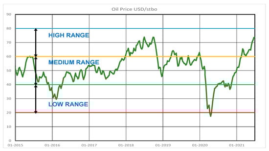
Figure 5.
Oil price range breakdown.
Applying the Integrated Workflow, for the four assumptions and three subintervals, the final table with the P50 results for the main business performance parameters is presented below (Table 6).
Table 6.
The profitable sub-cases.
Analyzing the data in the table, it can be observed that the vast majority of the profitable cases are based on the high oil price sub-segment, 60–80 USD/stbo. At this point, the field operator may decide to park the development of this field and save it for later or instead to explore other field development solutions and redo the whole Integrated Workflow.
Revision of Field Development Solution
The new development solution involves increasing the maximum liquid rates for the producers to 900 stb/d, water injection rates to 1200 stb/d and the field oil rate plateau to 10000 stbo/d. The advantage in this case is that the ESP pumps should not be changed if the maximum liquid rate is changed from 500 stb/d to 950 stb/d. In addition to this, eight low-production oil wells were removed, along with one water injector. Under the new development solution, the injector–producer ratio is 1:1.25, or four injectors maintaining five producers. The well economic limits were kept the same to make the two FDP solutions comparable. The condition of maintaining the field pressure above the bubble pressure must be satisfied in this case, too. As per the previous case, the field instantaneous VRR is maintained in the same range of 0.95 to 1.1.
Figure 6 shows the field performance under the new development strategy.
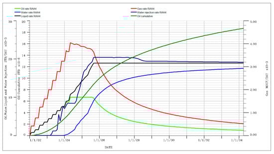
Figure 6.
New Field Development.
Under the current development solution, the field is attaining and maintaining a plateau of 10,000 stbo/d for almost 1.5 years. At the end of the twelve-year forecast, the field will produce 18.7 MMstbo, which corresponds to a recovery factor of 28.8%. The total water produced is 51.8 MMstb and the total injected water is 70.6 MMstb. As was the case with the previous FDP solution, a supplementary source of water is needed. Half of the required injection rate will be available from the produced water after 3.8 years.
Figure 7 shows the number of wells to be released annually for the optimized field development solution.

Figure 7.
Number of wells to be released annually.
Analysing Figure 7, it can be observed that the whole drilling program spans the first four years, and is aggressive in the second and third year (13 and 14 wells to be drilled and commissioned). This first and fourth years require the drilling and commissioning of four and eight wells, respectively.
At first, the economic model was run with wide ranges for the four assumptions, as defined in Table 4. The P50 values of the business performance indicators for a “most-likely” combination are presented in Table 7.
Table 7.
Table with Forecast Variables—Alternate Field Development Strategy.
Once more, oil is produced especially at the beginning of the field development. Even with large ranges for the four assumptions, the P50 values are showing a profitable solution.
As the next step, the authors prepared the 34 (81) cases—that is, all possible combinations—as per Table 5. The results can be seen in Table 8.
Table 8.
The Profitable Sub-Cases—Alternate Field Development.
Comparing Table 8 and Table 6, it can be observed that there are 47 (58%) profitable sub-cases. The encouraging aspect is that 20 (25%) sub-cases are based on a medium oil price interval. This makes the field development revised solution more attractive than the first proposed solution.
The workflow is not intended to be or to run as an optimizer. It does not consider maximizing or minimizing a forecast parameter, targeting one or more variables. Both the probabilistic economic model and the workflow are constructed to identify the input variables with the greatest influence on the forecast variables. If any of the input variables are defined with wide variation limits, by using the workflow, these limits can be divided into smaller intervals, resulting in several economic models, as combinations. Through individual assessment of each combination and by analysing the results, the user can better understand which combinations are profitable and under what conditions, and so decide the measures that will need to be taken.
5. Conclusions
Two ideas related to risk management in the oil industry were used:
- -
- (1) The analysis was performed for the upstream sector, in exploration and production portfolio management, in order to quantify the risk for each asset but also based on the interaction between assets. In this case, the asset refers to a well-defined oil field;
- -
- (2) Risk analysis aimed at integrating specific tools and corporate metrics (such as Net present value—NPV; Discounted cash flow return—DCF; Internal rate of return—IRR; Return of investment—ROI) in order to forecast the cumulative cash flow from a project and to inform a specific planning and decision process, with the aim of creating a long-term plan that can be used to forecast capital requirements for at least five years, the planning horizon matching the 12-year period for the asset under evaluation.
Analyzing the previous sections, it can be observed that main objective of the authors—to develop a risk management framework for the purpose of the economic performance analysis of a hydrocarbon field—was successfully achieved. The core part of this framework is a workflow (generic algorithm) which integrates petroleum engineering and petroleum economics. The workflow, called Integrated Workflow, is a partially automated and highly flexible method for evaluating probabilistically the economic performance of a hydrocarbon field development’s proposed solution. The Integrated Workflow (acting as a generic algorithm) is designed to be practical by addressing the real needs of oil and gas professionals, to be easy to use and easy to be repeated from one project to another.
The probabilistic economic model, designed and constructed by the authors, is highly complex (involving seventy-eight assumptions and twelve forecast variables) and was developed in Microsoft Excel using the worldwide industry-recognized probabilistic engine Oracle Crystal Ball.
The first field development solution (SOL_01) looks as though it is going to show negative most likely case (P50) profitability due to the relatively large limits of the four main influencers on profitability (cumulative DCF): oil price, drilling time, daily drilling rig cost, minimum water cut triggering the installation of artificial lift system (ESP).
Applying Integrated Workflow and setting up three subintervals of the four main influencers enumerated above, it has been observed that first field development solution was profitable only if the oil price limits corresponded to interval HIGH (60–80 USD/stbo). During the 6 ½ years (January 2015–June 2021) of oil price evolution history, oil prices above 60 USD/stbo were recorded only in 2018 and in the last three months of the first semester of 2021 (April–June).
This aspect revealed the importance of revising the field development solution and deriving the SOL_02 development case. The revision consisted in increasing the field oil rate plateau from 6500 stbo/d to 10,000 stbo/d by increasing the maximum produced liquid rate from 500 stb/d to 900 stb/d, by increasing the water injection rate from 1200 stbw/d to 1500 stbw/d and reducing the number of producing wells from 29 to 21 (eliminating the low performers) and the number of water injectors from 18 to 17 by stopping injectors that no longer provide support to producers.
The results were very promising: 58% of the total cases (81 cases in total) were profitable and 25% based on medium oil price range (MED interval 40–60 USD/stbo) were profitable.
To conclude, it can be stated that Integrated Workflow (as a useful tool for optimization of decisions regarding investments) proved to be very reliable, easy to use and easy to reapply. Based on the proposed framework, this workflow can be considered a great success.
This paper has aimed to focus on and fulfill several important goals:
- -
- Utilize a probabilistic economic model to determine the profitability of a development solution for a green field. The method can be adjusted to evaluate the profitability of rehabilitation of a mature oil field;
- -
- Identify the main parameters influencing the main economic indicators;
- -
- Treat the wide ranges of variation shown by the main influencing parameters. For example, the crude oil price per barrel is one of the most influential parameters on Discounted Cash Flow. Initially, the crude oil price is defined to vary from 20 to 80 USD/stbo. These limits are too wide to derive a reliable conclusion about the role played by the oil price, thus the initial interval was split into three intervals;
- -
- Provide a decision tool, as a workflow, to find the decisions that will drive a profitable field development solution.
In its present form, the Integrated Workflow is stable and error free. It was extensively tested to identify possible errors, and all the errors that were encountered were corrected. The authors are considering ways to further develop both the probabilistic economic model and the Integrated Workflow.
The directions of development for the probabilistic economic model are related to the various development solutions (gas injection, other artificial lift solutions, multiple well types (slant, high angles, horizontals, palm drilling, etc.)), different reservoir types (gas, oil with primary gas cap, condensate gas), diverse field location (on shore, offshore, remote locations, etc.) and by adding supplementary risks factors (H2S and NORM occurrences, political and regional factors, etc.).
The workflow can be improved by adding more subintervals for the most influential parameters and distribution types. Changing the numbers of subintervals from three to four will generate 44 (256) cases. Another direction for development will be to make the interface that is controlling the cases generator, submissions and results reader more user-friendly.
Author Contributions
Conceptualization, C.P. and S.A.G.; methodology, C.P. and S.A.G.; validation, C.P. and S.A.G.; formal analysis, C.P. and S.A.G.; investigation, C.P. and S.A.G.; writing—original draft preparation, C.P. and S.A.G.; writing—review and editing, C.P. and S.A.G. All authors have read and agreed to the published version of the manuscript.
Funding
This research received no external funding.
Institutional Review Board Statement
Not applicable.
Informed Consent Statement
Not applicable.
Data Availability Statement
Data sharing is not applicable to this article.
Conflicts of Interest
The authors declare no conflict of interest.
References
- Global 500. Fortune. Annual Ranking of the Top 500 Corporations Worldwide. Available online: https://fortune.com/global500 (accessed on 15 April 2021).
- Kaivo-oja, J.R.L.; Lauraeus, I.T. The VUCA Approach as a Solution Concept to Corporate Foresight Challenges and Global Technological Disruption. Foresight 2018, 20, 27–49. [Google Scholar] [CrossRef]
- Surbhi, A. Investment Decision Making in the Upstream Oil Industry: An Analysis. IUP J. Bus. Strategy 2015, 12, 40–52. [Google Scholar] [CrossRef]
- Cunha, J.C.S. Recent Developments in The Application of Decision Analysis for The Oil Industry. In Proceedings of the International Oil Conference and Exhibition in Mexico, Veracruz, Mexico, 27–30 June 2007. [Google Scholar] [CrossRef]
- Cunha, J.C. Risk Analysis Application for Drilling Operations. In Proceedings of the Canadian International Petroleum Conference, Calgary, AB, Canada, 8–10 June 2004. [Google Scholar] [CrossRef]
- Cunha, J.C.S.; Demirdal, B.; Ping, G. Use of Quantitative Risk Analysis for Uncertainty Quantification on Drilling Operations-Review and Lessons Learned. In Proceedings of the SPE Latin American and Caribbean Petroleum Engineering Conference, Rio de Janeiro, Brazil, 20–23 June 2005. [Google Scholar] [CrossRef]
- Lewis, D.; Guerrero, V.; Saeed, S.; Marcon, M.F.; Hyden, R. The Relationship between Petroleum Economics and Risk Analysis: A New Integrated Approach for Project Management. In Proceedings of the SPE/IADC Underbalanced Technology Conference and Exhibition, Houston, TX, USA, 11–12 October 2004. [Google Scholar] [CrossRef]
- Li, Z.X.; Liu, J.Y.; Luo, D.K.; Wang, J.-J. Study of Evaluation Method for the Overseas Oil and Gas Investment Based on Risk Compensation. Pet. Sci. 2020, 17, 858–871. [Google Scholar] [CrossRef]
- Manda, P.; Nkazi, D.B. The Evaluation and Sensitivity of Decline Curve Modelling. Energies 2020, 13, 2765. [Google Scholar] [CrossRef]
- Cheng, Y.; Wang, Y.; McVay, D.; Lee, W.J. Practical Application of a Probabilistic Approach to Estimate Reserves Using Production Decline Data. SPE Econ. Manag. 2010, 2. [Google Scholar] [CrossRef]
- Wang, H. What Factors Control Shale Gas Production and Production Decline Trend in Fractured Systems: A Comprehensive Analysis and Investigation. SPE J. 2017, 22, 562–581. [Google Scholar] [CrossRef] [Green Version]
- Boah, E.A.; Borsah, A.A.; Brantson, E.T. Decline Curve Analysis and Production Forecast Studies for Oil Well Performance Prediction: A Case Study of Reservoir X. Int. J. Eng. Sci. 2018, 7, 56–67. [Google Scholar]
- Tan, L.; Zuo, L.; Wang, B. Methods of Decline Curve Analysis for Shale Gas Reservoirs. Energies 2018, 11, 552. [Google Scholar] [CrossRef] [Green Version]
- Chang, C.; Li, Y.; Li, X.; Liu, C.; Fiallos-Torres, M.; Yu, W. Effect of Complex Natural Fractures on Economic Well Spacing Optimization in Shale Gas Reservoir with Gas-Water Two-Phase Flow. Energies 2020, 13, 2853. [Google Scholar] [CrossRef]
- McClure, M.; Picone, M.; Fowler, G.; Ratcliff, D.; Kang, C.; Medam, S.; Frantz, J. Nuances and Frequently Asked Questions in Field-Scale Hydraulic Fracture Modeling. In Proceedings of the SPE Hydraulic Fracturing Technology Conference, The Woodlands, TX, USA, 4–6 February 2020. [Google Scholar]
- Tripoppoom, S.; Xie, J.; Yong, R.; Wu, J.; Yu, W.; Sepehrnoori, K.; Miao, J.; Chang, C.; Li, N. Investigation of Different Production Performances in Shale Gas Wells Using Assisted History Matching: Hydraulic Fractures and Reservoir Characterization from Production Data. Fuel 2020, 267, 117097. [Google Scholar] [CrossRef]
- Tripoppoom, S.; Yu, W.; Sepehrnoori, K.; Miao, J. Application of assisted history matching workflow to shale gas well using EDFM and neural network -Markov Chain Monte Carlo algorithm. In Proceedings of the SPE/AAPG/SEG Unconventional Resources Technology Conference, Denver, CO, USA, 22–24 July 2019. [Google Scholar]
- Morales, A.; Holman, R.; Nugent, D.; Wang, J.; Reece, Z.; Madubuike, C.; Flores, S.; Berndt, T.; Nowaczewski, V.; Cook, S.; et al. Case Study: Optimizing Eagle Ford Field Development through a Fully Integrated Workflow. In Proceedings of the SPE Annual Technical Conference and Exhibition, Calgary, AB, Canada, 30 September–2 October 2019. [Google Scholar]
- Vătavu, S.; Lobonț, O.R.; Para, I.; Pelin, A. Addressing Oil Price Changes through Business Profitability in Oil and Gas Industry in the United Kingdom. PLoS ONE 2018, 13, e0199100. [Google Scholar] [CrossRef]
- Diaz, E.; Perez de Gracia, F. Oil Price Shocks and Stock Returns of Oil and Gas Corporations. Financ. Res. Lett. 2017, 20, 75–80. [Google Scholar] [CrossRef]
- Kang, W.; Perez de Gracia, F.; Ratti, R.A. Oil Price Shocks, Policy Uncertainty, and Stock Returns of Oil and Gas Corporations. J. Int. Money Financ. 2017, 70, 344–359. [Google Scholar] [CrossRef]
- Liu, J. Impact of Oil Price Changes on Stock Returns of UK Oil and Gas Companies: A Wavelet-Based Analysis. Available online: https://ssrn.com/abstract=2997025 (accessed on 15 April 2021).
- Al-Hemoud, A.; Al-Dousari, A.; Misak, R.; Al-Sudairawi, M.; Naseeb, A.; Al-Dashti, H.; Al-Dousari, N. Economic Impact and Risk Assessment of Sand and Dust Storms (SDS) on the Oil and Gas Industry in Kuwait. Sustainability 2019, 11, 200. [Google Scholar] [CrossRef] [Green Version]
- Al-Hemoud, A.; Al-Sudairawi, M.; Neelamanai, S.; Naseeb, A.; Behbehani, W. Socioeconomic Effect of Dust Storms in Kuwait. Arab. J. Geosci. 2017, 10, 18. [Google Scholar] [CrossRef]
- Adams, C.; Wilson, J.; Vandevelde, M. Moody’s Puts 175 Energy and Mining Companies on Downgrade Watch. Financial Times. 22 January 2016. Available online: https://www.ft.com/content/bfa6f25a-c0ea-11e5-9fdb-87b8d15baec2 (accessed on 10 April 2021).
- Díaz, A.; García-Donato, G.; Mora-Valencia, A. Quantifying Risk in Traditional Energy and Sustainable Investments. Sustainability 2019, 11, 720. [Google Scholar] [CrossRef] [Green Version]
- Ewing, B.T.; Malik, F.; Anjum, H. Forecasting Value-at-Risk in Oil Prices in the Presence of Volatility Shifts. Rev. Financ. Econ. 2018, 37, 341–350. [Google Scholar] [CrossRef]
- Lyu, Y.; Wang, P.; Wei, Y.; Ke, R. Forecasting the VaR of Crude Oil Market: Do Alternative Distributions Help? Energy Econ. 2017, 66, 523–534. [Google Scholar] [CrossRef]
- Cheng, C.; Wang, Z.; Liu, M.; Ren, X.-H. Risk Measurement of International Oil and Gas Projects Based on the Value at Risk Method. Pet. Sci. 2019, 16, 199–216. [Google Scholar] [CrossRef] [Green Version]
- Díaz, A.; García-Donato, G.; Mora-Valencia, A. Risk Quantification in Turmoil Markets. Risk Manag. 2017, 19, 202–224. [Google Scholar] [CrossRef]
- Emmer, S.; Kratz, M.; Tasche, D. What Is the Best Risk Measure in Practice? J. Risk 2015, 18, 31–60. [Google Scholar] [CrossRef] [Green Version]
- Zaroni, H.; Maciel, L.B.; Carvalho, D.B.; Pamplona, E.O. Monte Carlo Simulation Approach for Economic Risk Analysis of an Emergency Energy Generation System. Energy 2019, 172, 498–508. [Google Scholar] [CrossRef]
- Lux, T.; Segnon, M.; Gupta, R. Forecasting Crude Oil Price Volatility and Value-at-Risk: Evidence from Historical and Recent Data. Energy Econ. 2016, 56, 117–133. [Google Scholar] [CrossRef] [Green Version]
- Wang, Y.; Wu, C.; Yang, L. Forecasting Crude Oil Market Volatility: A Markov Switching Multifractal Volatility Approach. Int. J. Forecast. 2016, 32, 1–9. [Google Scholar] [CrossRef]
- Araújo Santos, P.; Fraga Alves, M.I. Forecasting Value-at-Risk with a Duration-Based POT Method. Math. Comput. Simul. 2013, 94, 295–309. [Google Scholar] [CrossRef]
- Zhang, D.; Ji, Q.; Kutan, A.M. Dynamic Transmission Mechanisms in Global Crude Oil Prices: Estimation and Implications. Energy 2019, 175, 1181–1193. [Google Scholar] [CrossRef]
- Ma, F.; Zhang, Y.; Huang, D.; Lai, X. Forecasting Oil Futures Price Volatility: New Evidence from Realized Range-Based Volatility. Energy Econ. 2018, 75. [Google Scholar] [CrossRef]
- Epelle, E.I.; Gerogiorgis, D.I. Adjoint-Based Well Placement Optimisation for Enhanced Oil Recovery (EOR) Under Geological Uncertainty: From Seismic to Production. J. Pet. Sci. Eng. 2020, 190, 107091. [Google Scholar] [CrossRef]
- Rahim, S.; Li, Z. Well Placement Optimization with Geological Uncertainty Reduction. IFAC-PapersOnLine 2015, 48, 57–62. [Google Scholar] [CrossRef]
- Jesmani, M.; Bellout, M.C.; Hanea, R.; Foss, B. Well Placement Optimization Subject to Realistic Field Development Constraints. Comput. Geosci. 2016, 20, 1185–1209. [Google Scholar] [CrossRef]
- Tavallali, M.S.; Karimi, I.A. Integrated Oil-Field Management: From Well Placement and Planning to Production Scheduling. Ind. Eng. Chem. Res. 2016, 55, 978–994. [Google Scholar] [CrossRef]
- Lee, S.; Landucci, G.; Reniers, G.; Paltrinieri, N. Validation of Dynamic Risk Analysis Supporting Integrated Operations across Systems. Sustainability 2019, 11, 6745. [Google Scholar] [CrossRef] [Green Version]
- Landucci, G.; Paltrinieri, N. Proactive Monitoring of Risk-Based Indicators: Example of Application in the Oil & Gas Integrated Operations. Available online: https://ntnuopen.ntnu.no/ntnu-xmlui/bitstream/handle/11250/2582865/HAZ28_099_full%2bpaper.pdf?sequence=3&isAllowed=y (accessed on 10 April 2021).
- Ahmadi, M.; Manera, M.; Sadeghzadeh, M. The Investment-Uncertainty Relationship in the Oil and Gas Industry. Resour. Policy 2019, 63, 101439. [Google Scholar] [CrossRef]
- Rack, V. Business Model Innovation in the Oil and Gas Supply Industry. Master Thesis, Nord University, Bodø, Norway, June 2017. [Google Scholar]
- Gheorghiu, S.A.; Popescu, C. Quantifying Economic Uncertainties and Risks in the Oil and Gas Industry. In Recent Applications of Financial Risk Modelling and Portfolio Management; Škrinjarić, T., Čižmešija, M., Christiansen, B., Eds.; IGI Global: Hershey, PA, USA, 2020; pp. 154–184. [Google Scholar] [CrossRef]
Publisher’s Note: MDPI stays neutral with regard to jurisdictional claims in published maps and institutional affiliations. |
© 2021 by the authors. Licensee MDPI, Basel, Switzerland. This article is an open access article distributed under the terms and conditions of the Creative Commons Attribution (CC BY) license (https://creativecommons.org/licenses/by/4.0/).