An Enhanced Distributed Voltage Regulation Scheme for Radial Feeder in Islanded Microgrid

Abstract

Even the simplest version of the distribution networks face challenges such as maintaining load voltage and system frequency stability and at the same time minimizing the circulating reactive power in grid-forming nodes. As the consumers at the far end of the radial distribution network face serious voltage fluctuations and deviations once the load varies. Therefore, this paper presents an enhanced distributed control strategy to restore the load voltage magnitude and to realize power-sharing proportionally in islanded microgrids. This proposed study considers the voltage regulation at the load node as opposed to the inverter terminal. At the same time, a supervisory control layer is put on to observe and correct the load voltage and system frequency deviations. This presented method is aimed at replacing paralleled inverter control methods hitherto used. Stability analysis using system-wide methodical small-signal models, the MATLAB/Simulink, and experimental results obtained with conventional and proposed control schemes verify the effectiveness of the proposed methodology.

1. Introduction

A reliable and stable distribution network represents a crucial aspect to successful power distribution to load demands. Suppling electrical power to loads can be enhanced using a well-organized distribution system [1,2]. Radial distribution networks (RDNs) are considered the most frequently employed distributed network [2,3]. RDNs are chains of conducting lines, which are divided into smaller branches for power delivery to customer’s premises. RDNs are more convenient than other configuration, as it is only fed at one end with low initial network cost. Moreover, it has easy circuit protection schemes to coordinate and design owing to its simplicity in establishing system component rating requirements [4]. As per the power network configuration, RDNs can be divided into three categories, i.e., “AC and DC networks”, “single-phase and three-phase networks”, and “balanced and unbalanced networks” [5]. Most of the developing countries use the AC distribution network as opposed to the DC network. Using DC distribution is a new technology, which requires fewer conductors for power dispersal, which reduces the line losses and cost of the conductors [6]. On the other side, the AC system could be either a single-phase or three-phase system [7]. A three-phase AC network can be further be classified as a balanced or unbalanced system: a balanced network contains the positive phase sequence components with equal magnitude and phase shift, while the unbalanced network has either a positive or negative sequence with irregular magnitude and phase shift. Unequal loading, fault, single-phasing, outrages, etc., are considered as the main causes of disturbances in the distribution system voltages and currents [8,9].

The conventional or renewable source of energy-based distributed generations (DGs) is the low-scale power generation network of wattage between a few kW to MW [10]. Power is provided in the system with respect to the power rating of DG and the identification of critical nodes. Over-voltage and over-current may occur without estimation of location and size of DG. DGs can be classified into four types, i.e., (1) injecting real and reactive power; (2) injecting real power and absorbing reactive power; (3) injecting real power solely; and (4) injecting only reactive power [10,11]. Microgrid (MG) is a cluster of different power sources, e.g., distributed generation units, storage units, microturbines, fuel cells, loads, etc. MG is suitable for the low voltage distribution side [12,13]. The primary task of MG is to deliver quality power without being suffered from voltage fall. The penetration of renewable sources such as fuel cells, PV cells into MG has reduced the fuel cost and CO₂ emission [14]. However, proper integration of such sources required the DC to AC inversion, where the setting of power converters and power flow control faces vital challenges. The suitable energy storage system with its control algorithm makes the power flow more efficient [14,15].

Participation of generating units into the grids defines the amount of power to be supplied [2]. The generating unit could also contribute from the distribution side as well. The mode of generation is basically based on the main and subsequent generating units available as a source of power [3,16]. It can be characterized as the centralized generation, where the power generation is controlled by the main power plants and grid. Moreover, depending on the controlling scheme of MG, it can be classified as central controlled MG and local controlled MG, where combination and lone generating units are controlled [11,15]. Depending on the power supply from the substation side, MG operation can be redefined as grid-dependent, where the MG exists in the network even when the main supply is provided from the substation [13]. MG puts its contribution in a grid-dependent radial distribution system when load demand exceeds and power quality goes down. Grid-independent or islanded, where the MG is the only source of power and network is free from the substation that can be occurred during outages. Mainly, MG gives the power during the excess demand in grid-dependent systems, minimizes loss, and maintains power quality [17,18]. It acts as a backup power source during the islanded mode of operation or gird failure situation, controls the loads, converts DC power into AC power, and promises security and protection [19,20].

The study on control of grid-forming units was first carried out in uninterruptible power supply systems with parallel operation [21,22,23]. In islanded MGs, the droop control schemes widely employ to obtain power sharing by using communication channels. Power-sharing control schemes of DG units based on communication are, master/slave [24,25,26], concentrated control [25,27,28] and distributed control [29]. Oppositely the control methodologies without using the communication channel are mainly on the droop idea, which includes four leading categories: (1) virtual framework structure-based scheme [30,31,32,33,34,35]; (2) signal injection strategy [36]; (3) conventional and variants of the droop control [37,38,39,40,41,42,43] and (4) “construct and compensate”-based schemes [37,39,44]. Integrated control schemes refer to hierarchical structures consists of primary, secondary, and tertiary control [45]. The work of primary control layers is to maintain the system voltage and frequency and offer the plug-and-play capability of DGs in MG. The secondary control layers use to correct the voltage and system deviations in order to improve the power quality, while the tertiary control employs to interact with the main grid [46].

In this paper, an effort has been made to enhance voltage regulation in radial feeders, usually employed in an islanded MG distribution network. The electric power generated from various DG units is not used efficiently by the end-users in the world as the consumers at the far end of the distributor face serious voltage fluctuations and deviations once the load varies. In this study, the two DG units are connected to MG through interfacing power inverters. Droop control scheme of parallel-connected inverters is employed at consumers end as opposed to inverter terminal. In islanded mode, the inverter droop control should regulate the user voltage, system frequency, and share-power proportionally. Further, the major contributions of this work are listed below,

• An enhanced distributed control scheme is presented, which can be used for a limited number of grid-forming nodes;
• A distributed secondary control layer is employed to restore the load voltage and frequency deviations. Modeling and analysis of an autonomous operation of inverter-based MG being verified through stability analysis using system-wide mathematical small-signal models;
• MATLAB/Simulink and experimental results are discussed with a comparison of conventional control schemes under load disturbances.

The remainder of this paper is organized as follows. Section 2 presents the operation principle of the system used in this proposed study. Section 3 outlines the derivations of the small-signal model for this MGs system with the employed controls. Section 4 elaborates the stability analysis of the system under the discussed controls. Further, it also presents the simulation and experimental results in detail with a comparison of the conventional and proposed control scheme, and Section 5 concludes the paper.

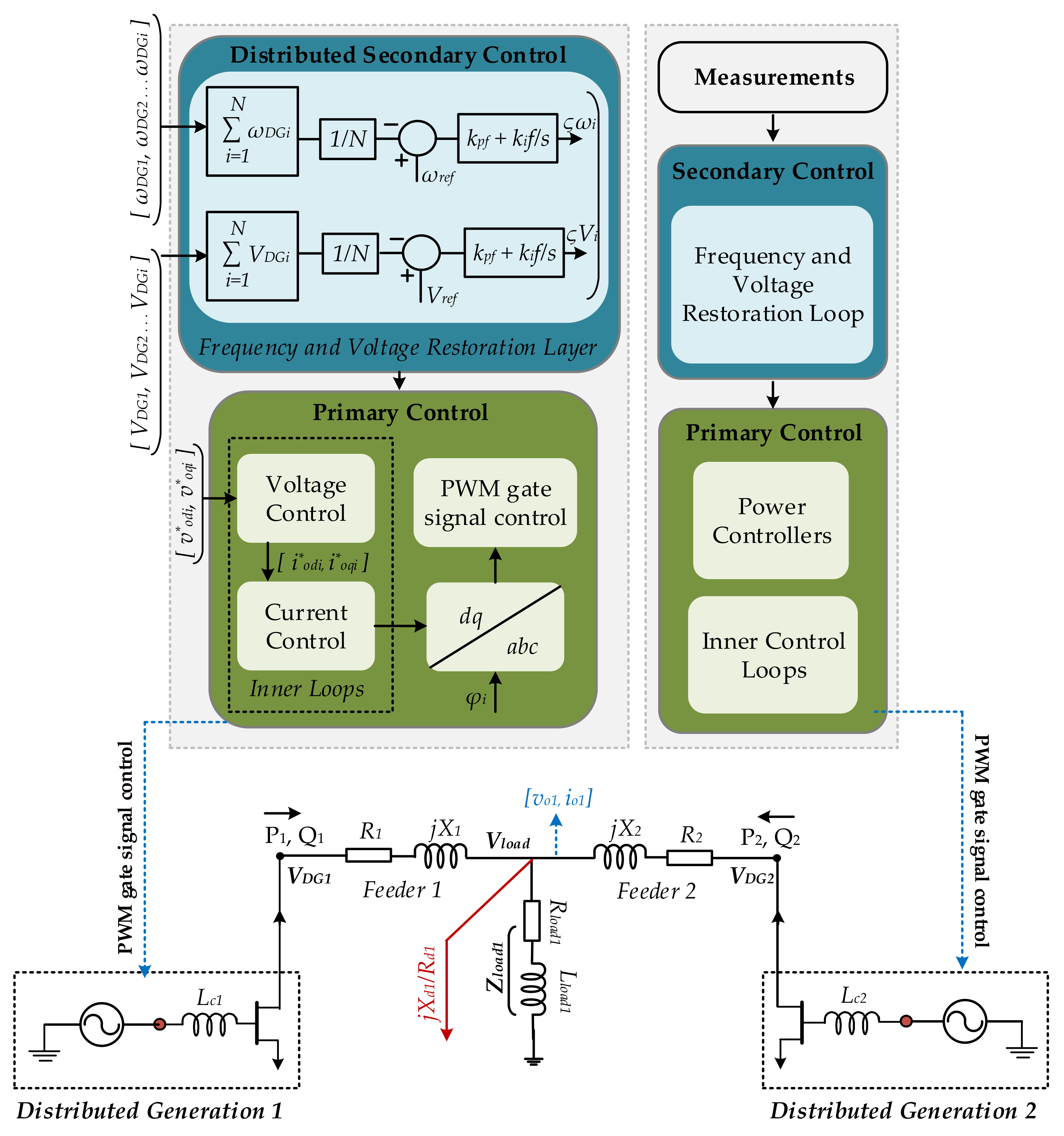
2. Proposed Control Strategy

This section presents the MG setup used in this proposed study. To adequately describe the proposed control scheme, we systematically go about describing the mathematical model and power flow control along with the necessary mathematical representations.

2.1. Microgrid Power Network Model

A radial distribution network with a three-phase, three-wire configuration is used in this study, as shown in Figure 1. Power converters and RL load are connected through feeder 1 and feeder 2. This network can work autonomously in an “islanded” mode.

Table 1. System parameters for stability analysis and experimental prototype.

Sr. No.	Control Parameters for Stability Analysis
1	Droop Gains	Min	Max
	mP	0.02	0.32
2	Consensus frequency
	kpf	0.45	-
	kif	4.5 × e−04	-
3	Consensus voltage
	kpV	0.3	2.5
	kiV	0.08	0.48
4	Time delay
	τdelay	0	6 × e−03
Sr. No.	Control Parameters for Experimental Prototype
	Components	Units	Components	Units
1	Operating frequency	50 Hz	Sampling rate	1 ms
2	DG units ratings	3 A, 30 V	jXi1, jXi2	200 uH
3	jXc1, jXc2	20 uF	jXg1, jXg2	60 uH
4	Lline1/Rline1	2 mH/0.2 Ω	Lload/Rload	2 mH/10 Ω
5	Lline2/Rline2	2 mH/0.2 Ω	Ld1/Rd1	1 mH/5 Ω

and

Table 2. System parameters for simulations.

Sr.	Components	Units	Components	Units
1	Nominal frequency	50 Hz	Lload/Rload	80 mH/60 Ω
2	Simulations Vref	300 V	Ld1/Rd1	10 mH/20 Ω
3	Lline1/Rline1; Lline2/Rline2	2 mH/0.2 Ω; 2 mH/0.2 Ω	Switching-Frequency	16 kHz

express the rated system parameters for stability analysis, simulation, and experimental prototype. In this study, load voltage magnitude restoration is considered unlikely the voltage regulation at the inverter terminal. By using the reference frame transformation, the load voltage is transformed into d-q axis components. Based on such sensed measurements at ith node of each inverter, the apparent power S is calculated and dispatched to droop controllers of every ith inverter via low-pass filters. Depending on the received information, the droop controllers further send the reference voltage command to inner voltage and current layers. Distributed secondary layer periodically corrects the load voltage and system frequency deviations.

2.2. Mathematical Model

To understand the varying power relationship corresponding to change in amplitude and frequency, the complex power delivered to the ith ac bus is expressed in term of network voltages and admittances. The complex power delivered to the ith bus can be expressed as:

$$S_i=V_i{I}_i^{*}$$

(1)

Applying the algebraic multiplication to Equation (A6) shown by Appendix A and then collecting the real part P_i and imaginary part Q_i results:

$$P_i={\displaystyle \sum _{j=1}^N \left|V_i\right|\left|V_j\right|\angle \left(G_i{}_j\cos ({\phi }_i-{\phi }_j)+B_{ij}\sin ({\phi }_i-{\phi }_j)\right)}$$

(2)

$$Q_i={\displaystyle \sum _{j=1}^N \left|V_i\right|\left|V_j\right|\angle \left(G_i{}_j\sin ({\phi }_i-{\phi }_j)-B_{ij}\cos ({\phi }_i-{\phi }_j)\right)}$$

(3)

Power angle φ in medium-voltage lines are small, assuming sinφ = φ and cosφ =1, the Equations (2) and (3) re-expressed:

$$P_{i,R_x=0}\approx \frac{V_i{V}_j}{X_i}[ \sin {\phi }_{ij}]$$

(4)

$$Q_{i,R_x=0}\approx \frac{V_i^2-V_i{V}_j\cos {\phi }_{ij}}{X_i}$$

(5)

where the mathematical expression of term φ_ij and (V_i − V_j) is given in Appendix B. Equations (4) and (5) illustrates a direct relationship among the real power P_i and power angle φ as well as between the reactive power Q_i and voltage difference V_i − V_j.

2.3. Power Flow Control

DC power source is connected with the ith inverter bridge, and its output voltage and frequency are adjusted by the power controller and inner voltage and current controllers. All the operating DG units within the system are individually formulated in their d-q frame, which is based on their angular frequency ω_i and angle φ_i. Power electronics inverters interfaced among each DG unit and grid are converted to the d-q frame by using transformation equation as follows:

$$\left[\begin{array}{c}{f}_D\\ f_Q\end{array}\right]=\left[\begin{array}{cc}\begin{array}{c}\cos (\phi i)\\ \sin (\phi i)\end{array}& \begin{array}{c}-\sin (\phi i)\\ \cos (\phi i)\end{array}\end{array}\right]\left[\begin{array}{c}{f}_d\\ f_q\end{array}\right]$$

(6)

The angle of ith DG unit’s d–q fame can be written:

$${\phi }_i={\displaystyle \int (\xi {\omega }_i})dt$$

(7)

Droop control-based power controller block is shown in Figure 2a. Its purpose is to dispatch the voltage reference v∗_odi and v∗_oqi to inner control layers. Average output powers (P_i, Q_i) are obtained from instantaneous power passing low-pass filters, where the instantaneous real P and reactive Q power in the d-q rotating frame can be written as p_i = v_odi.i_odi+ v_oqi.i_oqi and q_i = v_odi.i_oqi+ v_oqi.i_odi. On individual frame d-q, v_odi, v_oqi, i_odi and i_oqi are the load voltage and line current of an ith inverter. Droop strategy demonstrates the relationship among the active power and system frequency p-ω, and between the reactive power and feeder load node voltage magnitude Q-V, can be illustrated as, ω_i = ω_ref − m_PiP_i and v*_odi = V_ref − n_QiQ_i, where ω_ref, V_ref, m_Pi and n_Qi are nominal frequency, voltage and droop coefficients, respectively, of each ith DG unit. Further, the reference voltage to the inner voltage layer is denoted by v*_odi. Q-V droop control strategy by considering the load node voltage magnitude can be written by (8), illustrated in Figure 2a.

$$v{*}_{odi}=V_{ref}-n_{Qi}{Q}_i$$

(8)

where V_ref is the nominal voltage of all inverters, while v*_odi is responsible for restoring the feeder load node load voltage, which regulates the voltage deviation caused by the droop controllers.

2.4. Distributed Secondary Control Layer: Voltage and Frequency Regulation

Distributed secondary control layers are used to restores the voltage and frequency deviations as the strategy expressed by Equations (9) and (10).

$$\left.\begin{array}{l}\overline{{\omega }_{avg}}=\frac{{\displaystyle \sum _{i=1}^N{\omega }_{DGi}}}{N}\\ {\omega }_i=({\omega }_{ref}-\overline{ {\omega }_{avg}})\\ \varsigma {\omega }_i=k_{pf}{\omega }_i+k_{if}{\displaystyle \int {\omega }_{i}dt}\end{array}\right)$$

(9)

where the ω_ref is the reference frequency, ω_DGi is the measured system frequency that is being sensed at all the nodes of ith inverters. The frequency correction term ςω_i is sent to the frequency reference of each ith inverter shown in Figure 1. K_pf and K_if are the proportional and integral gains for controllers.

Load voltage regulations schemes can be expressed as:

$$\left.\begin{array}{l}\overline{V_{avg}}=\frac{{\displaystyle \sum _{i=1}^N{V}_{DGi}}}{N}\\ V_i=(V_{ref}-\overline{ V_{avg}})\\ \varsigma V_i=k_{pf}{V}_i+k_{if}{\displaystyle \int V_{i}dt}\end{array}\right)$$

(10)

where V_ref and V_DGi are the nominal reference voltage and measured system voltage, respectively, in d-axis, which is sensed at each inverter’s nodes. K_pf and K_if are the proportional and integral gains for controllers. The updated voltage correction ςω term is applied to the voltage reference of each ith inverter.

3. Small-Signal Analysis of the Microgrid System

Intermittent latencies and delay of component communication links may result in power imbalances between generation sources, deviations in node voltages, and system frequency. Therefore, the stability of the system is analyzed by variations in P-f droop gain m_P and communication delay T_d. The small-signal modeling strategy is based on three important sub-modules, which are the inverter, network, and loads. State equations of the network and the connected loads with any ith DG inverter are presented in the reference frame by using the transformation strategy.

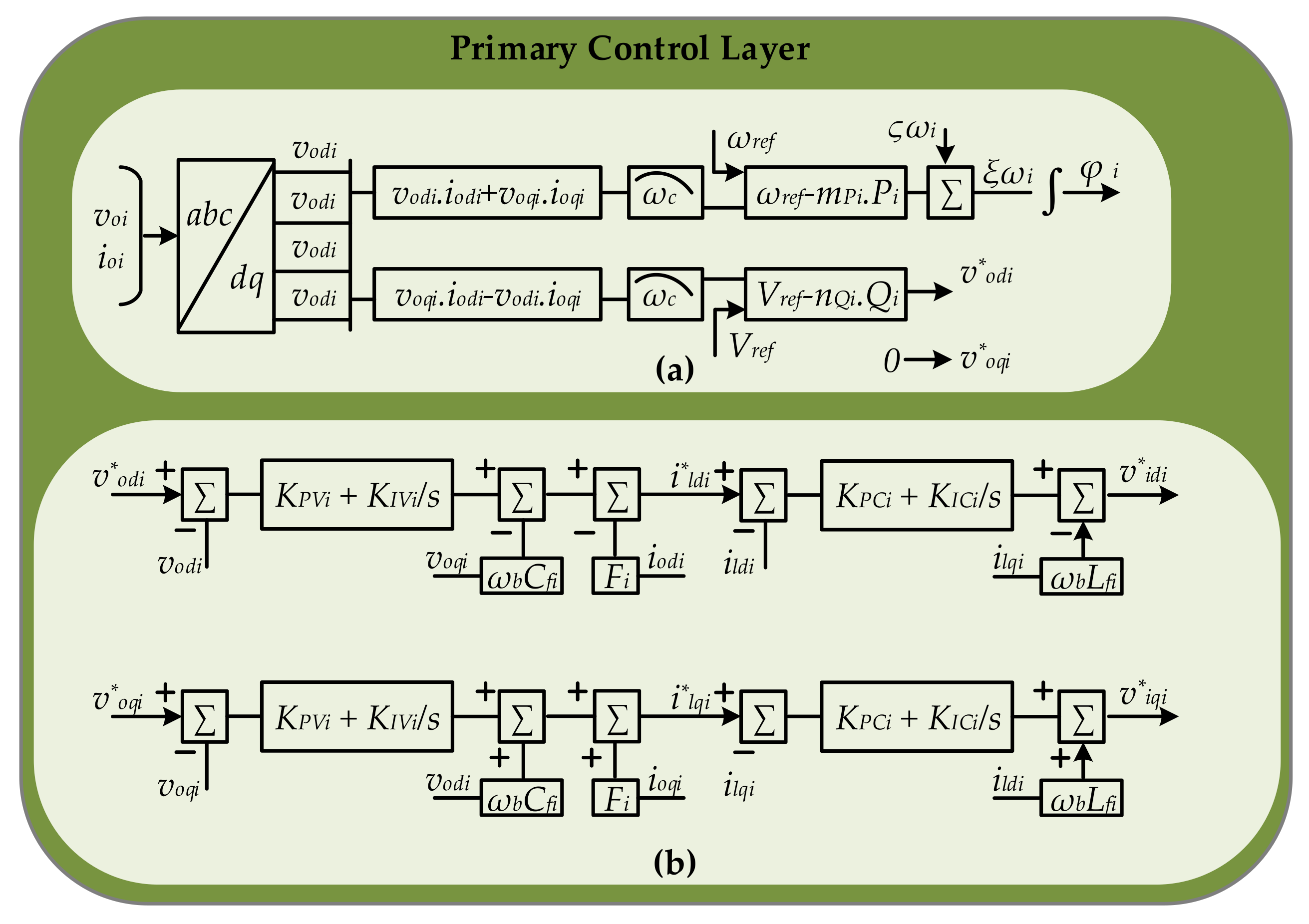
3.1. Primary Controller

From measured output current and voltage, the instantaneous power can be written as p = v_odi.i_odi + v_oqi.i_oqi and q = v_odi.i_oqi − v_oqi.i_odi. The small signal modeled for active power can be obtained as given in (11) by linearization.

$$\dot{\Delta }{P}_i=-{\omega }_{ci}.\Delta P_i+{\omega }_{ci}(I_{odi}\Delta v_{odi}+I_{oqi}\Delta v_{oqi}+V_{odi}\Delta i_{odi}+V_{oqi}\Delta i_{oqi})$$

(11)

$$v_{odqi}={\left[\begin{array}{cc}{v}_{odi}& v_{oqi}\end{array}\right]}^T, i_{odqi}={\left[\begin{array}{cc}{i}_{odi}& i_{oqi}\end{array}\right]}^T$$

(12)

Algebraic modeling for the voltage controller and the current controller can be expressed as follows,

$${i*}_{ldi}=F_i.v_{odi}-{\omega }_b.C_{fi}.\Delta v_{oqi}+K_{PVi}({v*}_{odi}-{v*}_{odi})+K_{IV}{}_i{\phi }_{di}$$

(13)

$${i*}_{lqi}=F_i.v_{oqi}+{\omega }_b.C_{fi}.\Delta v_{oqi}+K_{PVi}({v*}_{oqi}-{v*}_{oqi})+K_{IV}{}_i{\phi }_{qi}$$

(14)

$${v*}_{idi}=-{\omega }_b.L_{fi}.i_{lqi}+K_{PCi}({i*}_{ldi}-i_{ldi})+K_{IC}.{\gamma }_{di}$$

(15)

$${v*}_{iqi}={\omega }_b.L_{fi}+K_{PCi}({i*}_{lqi}-i_{lqi})+K_{IC}.\Delta {\gamma }_{qi}$$

(16)

The small-signal state-space modeling for voltage and current loop is given in Appendix D.

3.2. Grid Side Filter Model

The small-signal model of LC output filter and coupling inductance by assuming that voltage provided by the inverter is the same as demand voltage is expressed as in (17)–(19).

$$\frac{d{i}_{ldqi}}{dt}=-\frac{R_{fi}}{L_{fi}}.i_{ldqi}+{\omega }_i.i_{ldqi}+\frac{1}{L_{fi}}.v_{idqi}-\frac{1}{L_{fi}}.v_{odqi}$$

(17)

$$\frac{d{v}_{odqi}}{dt}={\omega }_i.v_{oqqi}+\frac{1}{C_{fi}}.i_{ldqi}-\frac{1}{C_{fi}}.i_{odqi}$$

(18)

$$\frac{d{i}_{odqi}}{dt}=-\frac{R_{ci}}{L_{ci}}.i_{odqi}+{\omega }_i.i_{odqi}+\frac{1}{L_{ci}}.v_{odiq}-\frac{1}{L_{ci}}.v_{obdqi}$$

(19)

The LC filter and coupling inductance, their linearization small-signal equations are represented by Appendix E.

3.3. Complete Model of an ith Inverter

The output variables need to the converter in a common reference frame to connect at ith inverter with the rest of the system. In our case, the output currents are the output variables of ith inverters, which can be expressed in vector form ∆i_odqi. ∆io_DQi, which is a small-signal output current, can be expressed by Appendix E.1. The bus voltage on the common reference frame is the input signal to the ith inverter model. Therefore, by using reverse transformation, the bus voltage can be converted into an ith individual inverter reference frame.

$$[\Delta u_{bdq}]=[T{\gamma }^{-1}].[\Delta u_{bDQ}]+[T_{\sigma }{}^{-1}][\Delta \delta ], \mathrm{where}, T_{\sigma }{}^{-1}=\left[\begin{array}{l}-U_{bD}\sin (\delta )+U_{bQ}\cos (\delta )\\ -U_{bD}\cos (\delta )-U_{bQ}\sin (\delta )\end{array}\right]$$

(20)

By combining the aforementioned state-space models for three controllers of an ith inverter, which are power controller, voltage controller and current controller, and output grid side LCL filter, the complete small-signal model can be obtained.

$$[\Delta {\dot{x}}_{invi}]=A_{invi}.[\Delta x_{invi}]+B_{invi}.[\Delta u_{bDQi}]+B_i{\omega }_{com}.[\Delta {\omega }_{com}]$$

(21)

$$\left[\begin{array}{c}\Delta {\omega }_i\\ \Delta i_{o}DQ\end{array}\right]=\left[\begin{array}{c}Cinv\omega i\\ Cinvci\end{array}\right].[\Delta x_{invi}]$$

(22)

where

$$[\Delta x_{inv}]={\left[\Delta {\delta }_i\Delta P_i\Delta Q_i\Delta {\phi }_{di}\Delta {\phi }_{qi}\Delta {\gamma }_{di}\Delta {\gamma }_{qi}\Delta i_{ldi}\Delta i_{lqi}\Delta v_{odi}\Delta v_{oqi}\Delta i_{odi}\Delta i_{oqi}\right]}^T$$

The matrices A_invi, B_invi, B_iwcom, C_invwi, and C_invci are the system matrices described by Appendix C.

3.4. Combined Model of N Inverters

In MG, the N number of DG inverters may be operating as a source at variable distances among each other. In this section, our approach is to discuss the possible sub-model form of all individual ith to k^th DG inverters and combine them with the existing corresponding network. The combined small-signal model of the “N” number of DG inverters is expressed by:

$$[\stackrel{.}{\Delta x_{inv}}]=A_{inv}.[\Delta x_{inv}]+B_{inv}.[\Delta v_{bDQ}]$$

(23)

$$[\Delta i_{oDQ}]=C_{invc}.[\Delta x_{inv}]$$

(24)

where the system matrices are given by Appendix F.

3.5. Network and Load Model

If an ith feeder line is connected between node j and k, mathematical modeling can be presented as follows.

$$\frac{\mathrm{d}{i}_{\mathrm{lineDi}}}{dt}=-\frac{R_{linei}}{L_{linei}}{i}_{lineDi}+\omega i_{lineQi}+\frac{1}{L_{linei}}{v}_b{D}_j-\frac{1}{L_{linei}}{v}_b{D}_k$$

(25)

$$\frac{\mathrm{d}{i}_{\mathrm{lineQi}}}{dt}=-\frac{R_{linei}}{L_{linei}}{i}_{lineQi}-\omega i_{lineDi}+\frac{1}{L_{linei}}{v}_b{Q}_j-\frac{1}{L_{linei}}{v}_b{Q}_k$$

(26)

$$[\stackrel{.}{\Delta i_{lineDQ}}]=A_{LINE}.[\Delta i_{lineDQ}]+B_{1LINE}.[\Delta u_{bDQi}]+B_{2LINE}.\Delta \omega$$

(27)

where

$$[\stackrel{.}{\Delta i_{lineDQ}}]={[\Delta i_{lineDQ}{}_1 \Delta i_{lineDQ2}\dots \Delta i_{lineDQ}n]}^T,[\Delta u_{bDQi}]={[\Delta i_{bDQ}{}_1 \Delta i_{bDQ2}\cdots \Delta i_{bDQm}]}^T,\Delta \omega =\Delta {\omega }_{com}$$

The matrices A_LINE, B_1LINE, B_2LINE, A_LINEi, B_2LINEi, and B_1LINEi are the system matrices given in Appendix F.1. If there are p load points available in a particular network, then the small-signal model can be presented as,

$$[\stackrel{.}{\Delta i_{loadDQ}}]=A_{LOAD}.[\Delta i_{loadDQ}]+B_{1LLOAD}.[\Delta u_{bDQi}]+B_{2LOAD}.\Delta {\omega }_i$$

(28)

$$[\Delta i_{loadDQ}]={[\Delta i_{loadDQ1 }\Delta i_{loadDQ2\cdots }\Delta i_{loadDQ p}]}^T$$

where A_LOAD, B_1LOAD, B_2LOAD, A_LOADi, and B_1LOADi are the system matrices described in Appendix G.

3.6. Complete Microgrid Model

It can have observed that the node voltages are used as inputs to every subsystem. In the assurance of well-defined node voltage, a virtual resistor r_N is supposed among all m nodes and grounds, which symbolic form can be defined as

$$[\Delta v_{bDQ}]=R_N(M_{INV}[\Delta i_{oDQ}+M_{load}[\Delta i_{loadDQ}]+M_{NET}[\Delta i_{lineDQ}])$$

(29)

The diagonal elements of matrix R_N is equal to r_N, which has a size of 2 m * 2 m matrix. The mapping matrix M_INV and M_load are the size of 2 m * 2 m and 2 m * 2 p, respectively. M NET matrix maps the connecting transmission lines onto the network nodes having a size of 2 m * 2 n. Finally, the complete MG small-signal model is given by Equation (30).

$$\left[\begin{array}{c}\stackrel{.}{\Delta x_{inv}}\\ \Delta i_{lineDQ}\\ \Delta i_{loadDQ}\end{array}\right]=A_{MG}\left[\begin{array}{c}\Delta x_{inv}\\ \Delta i_{lineDQ}\\ \Delta i_{loadDQ}\end{array}\right]$$

(30)

where A_MG is the state matrix and given as

$$A_{MG}=\left[\begin{array}{ccc}{A}_{inv}+B_{inv}{R}_N{M}_{inv}{C}_{invc}& B_{inv}{R}_N{M}_{NET}& B_{inv}{R}_N{M}_{load}\\ B_{1NET}{R}_N{M}_{inv}{C}_{invc}+B_{2LINE}{C}_{inv\omega }& A_{LINE}+B_{1LINE}{R}_N{M}_{NET}& B_{1LINe}{R}_N{M}_{load}\\ B_{1LOAD}{R}_N{M}_{inv}{C}_{invc}+B_{2LOAD}{C}_{inv\omega }& B_{1LOAD}{R}_N{M}_{NET}& A_{load}+B_{1LOAD}{R}_N{M}_{load}\end{array}\right]$$

(31)

4. Results and Discussion

In this section, the stability analysis, simulation, and experimental results for power sharing, voltage, and frequency regulation, are discussed. The simulations on MATLAB/Simulink are conducted on circuit configuration given in Figure 1 for three-phase 50 Hz islanded MG wherein the two paralleled connected DG1 and DG2 are connected to the RL load via feeder impedance X1–R1 and X2–R2. Moreover, the photo of the lab-scaled experiment hardware is illustrated in Figure 3. System and controller parameters that have been used in conventional and proposed control schemes are shown in Table 1 and Table 2.

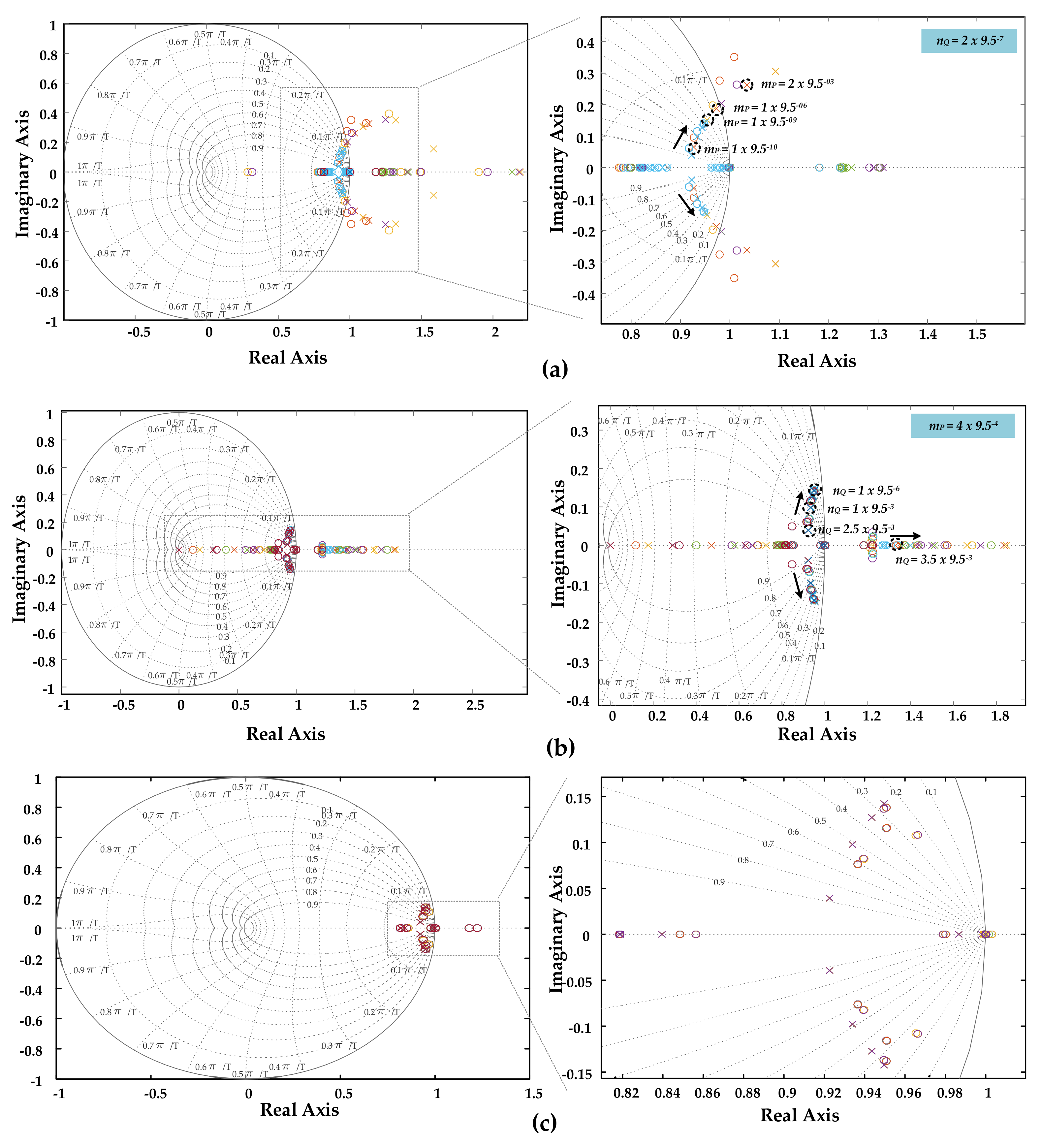
4.1. Modeling Results

The complete model of the test system under the proposed control scheme is achieved and used to analyze the stability of the system under varying communication latencies and control gains. MATLAB/Simulink and linear analysis tools have been used to obtain modeling results by analyzing this complex system through perturbing dynamical equations. Figure 4a,b shows the stability plot for the proposed control framework by varying real power droop gain m_P to trace the network trajectory. The control values of the droop gain m_P where system poles appear to be in the vicinity of the unit origin are maximum allowable limits. Therefore, using the poles zero evolutions, the control gain sensitivity and system stability are predicted. The maximum and minimum m_P gain values used for the proposed control scheme are 1 × 9.5⁻⁹ and 1 × 9.5⁻⁵, respectively.

Figure 4c demonstrates the pole and zero traces resulting from the behavior of the MG system by varying the time delays with the proposed control scheme. Movement of system poles is captured by starting with time delay t_d = 0 and increasing it step by step to a maximum time delay of t_d = 3 s. Poles are observed in the stable region for the time delay values 0 > td < 1 s and outside the unit circle for the td > 1 s, which makes the MG system divergent and unstable.

4.2. Simulation Results

In this section, the MATLAB/Simulink-based results obtained with conventional and proposed control strategies are discussed. The simulation verifications are composed of two cases. Case 1 outlines the results obtained with a conventional control scheme, while case 2 validates the effectiveness of the proposed control strategy. The initial conditions and control parameters as shown by Table 1 and Table 2 are the same for both cases.

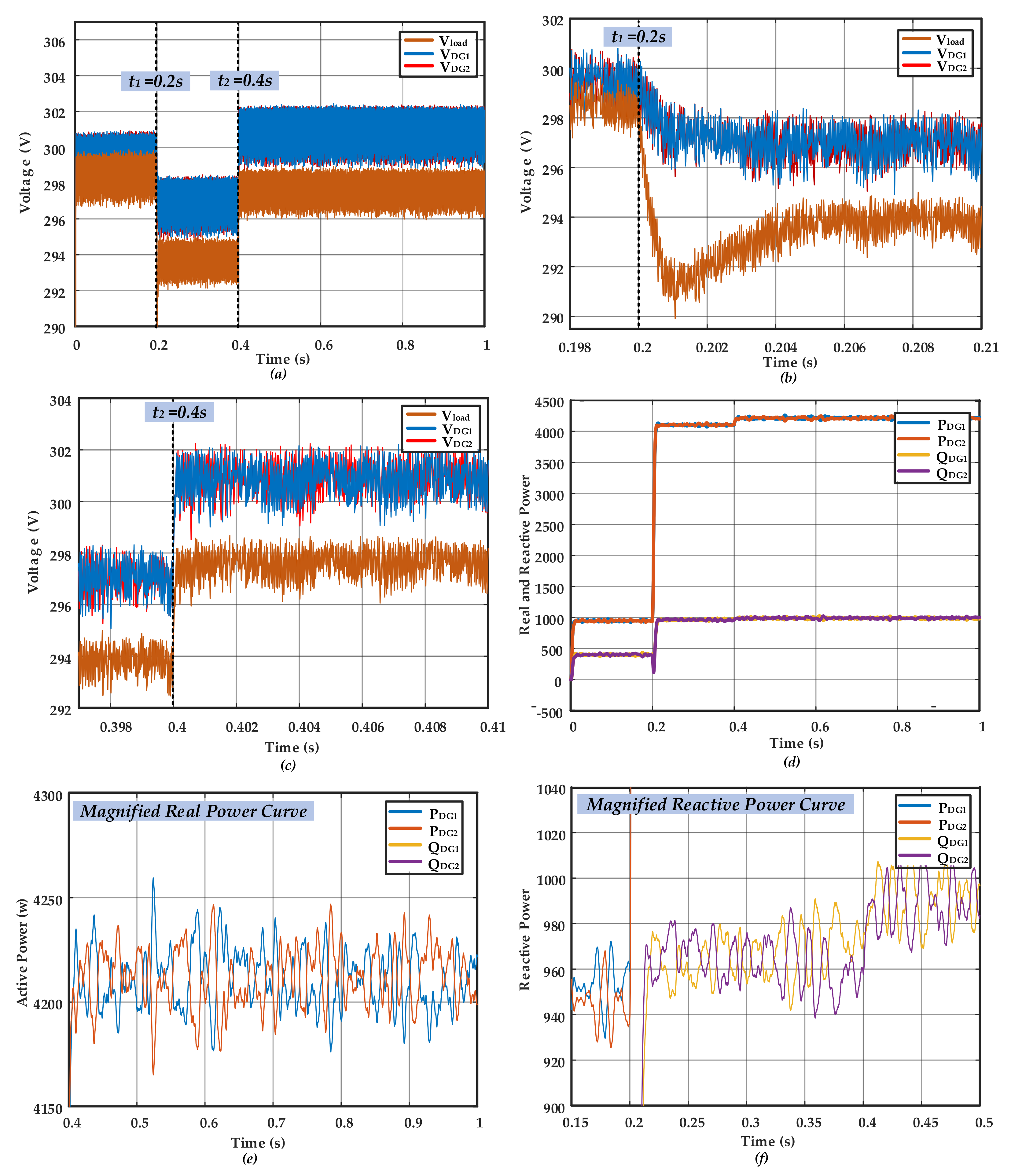
4.2.1. Case 1: MATLAB/Simulink Results with Conventional Control Strategy

Figure 5 shows the results obtained with a conventional control scheme. The objective of this scheme is to hold the load voltage at its original state, i.e., V_ref = 300 V, in the presence of load disturbance. To examine the methodology, the disturbance load (L_d1 = 10 mH, R_d1 = 20 Ω) is exerted at time t₁, and later the conventional control scheme is activated at the time t₂. Figure 5a illustrates the load voltage deviation of 2 V even the load disturbance is not yet exerted. This load voltage further deviates and is set at 393.5 V once the disturbance load is added at time t_1, as shown by Figure 5b. The load voltage drop of 4.5 V is removed once the conventional control strategy is activated at t₂. Although the conventional scheme is activated, still 2.3 V load voltage deviation is observed, as shown by Figure 5c. Real and reactive power sharing is illustrated by Figure 5d, while Figure 5e,f show the magnified results of real and reactive power, respectively.

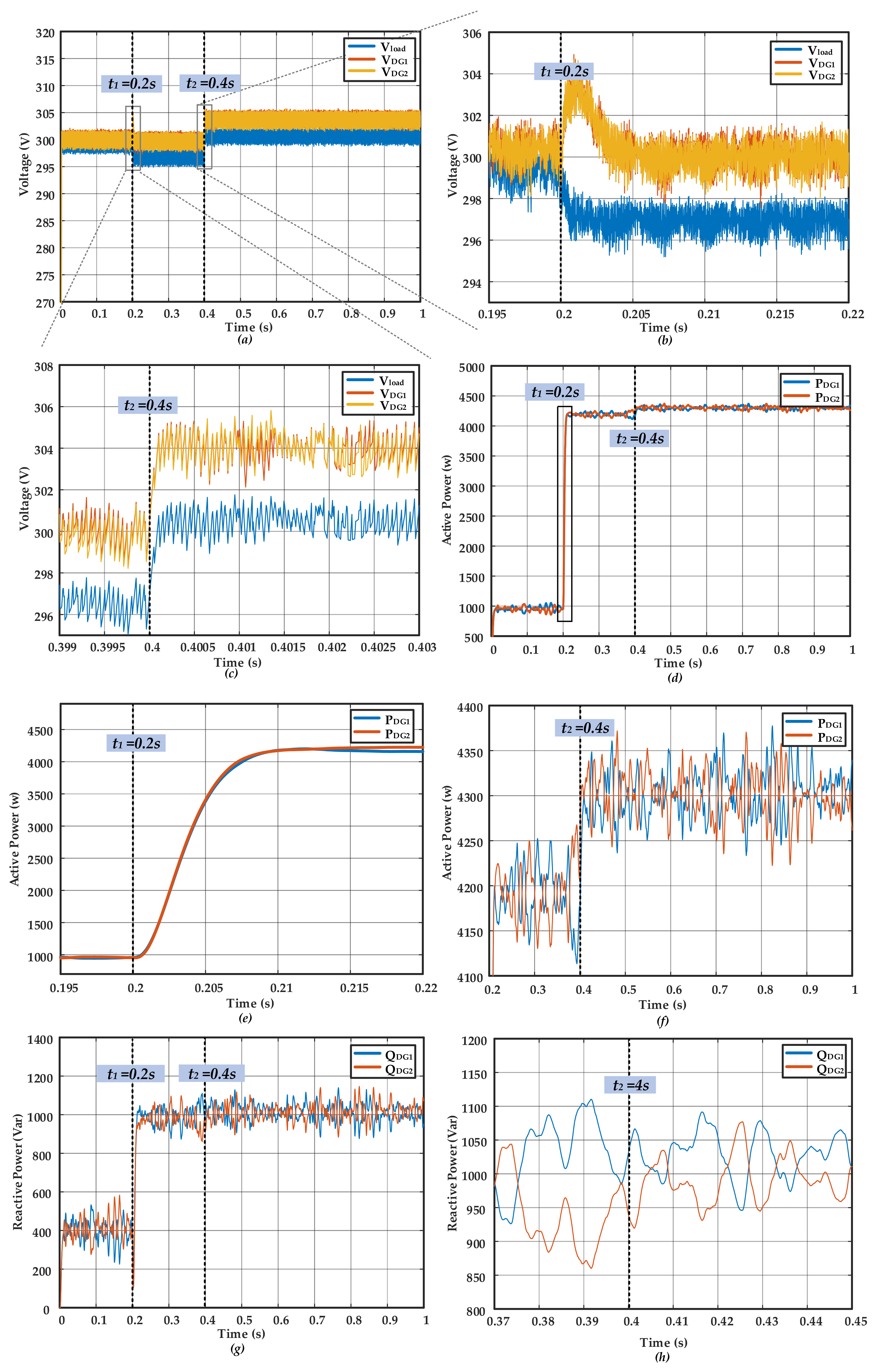
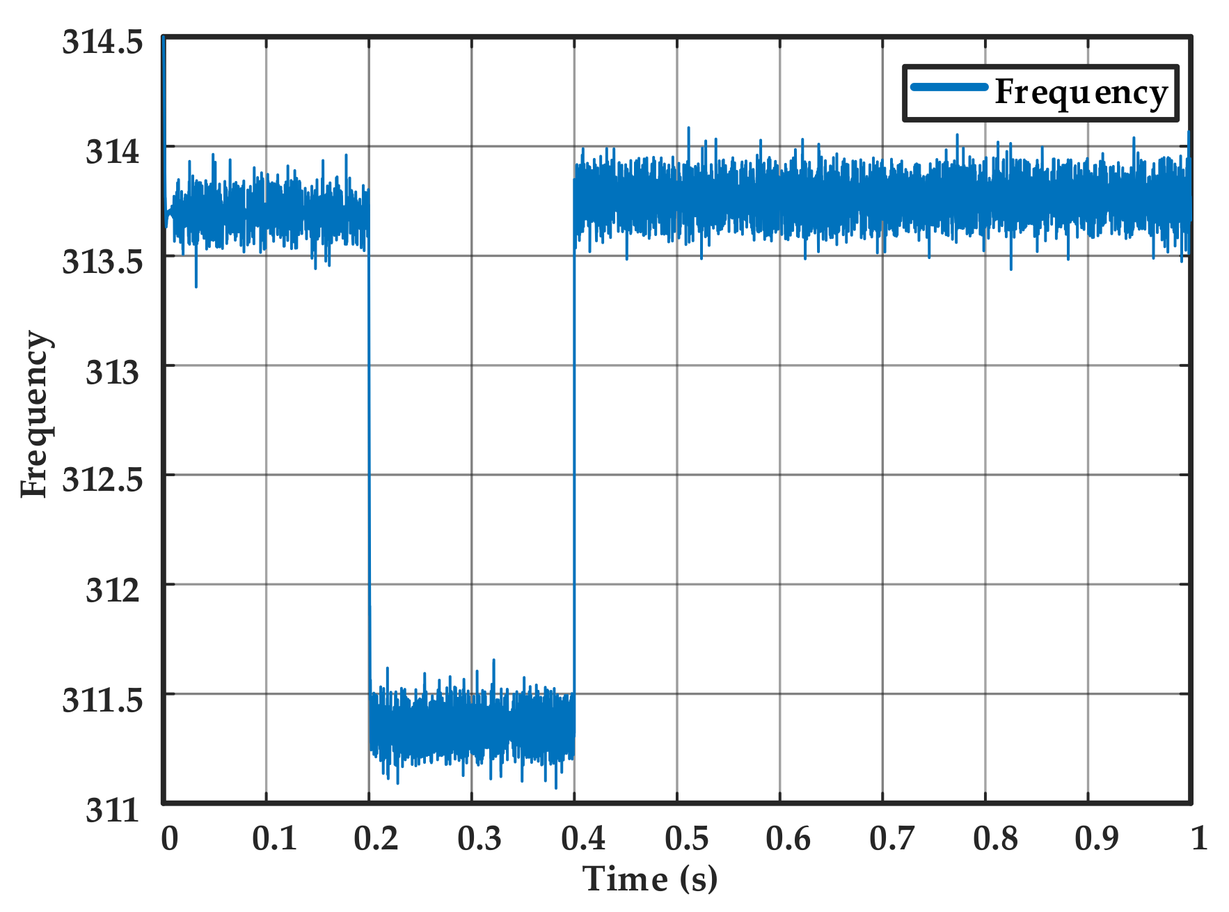
4.2.2. Case 2: MATLAB/Simulink Results with Proposed Control Strategy

Figure 6 shows the results obtained with the proposed control scheme. As opposed to the conventional scheme, the initial load voltage is observed at the desired value, i.e., V_ref = 300 V, as shown by Figure 6a. Once the disturbance load jX_d1/R_d1 is exerted at t₁, an obvious 3 V load voltage drop is depicted, as illustrated by Figure 6b. The proposed control scheme is activated at t_2, as shown in Figure 6c, where load voltage has resorted to nearly its original state. Figure 6d,g show the real and reactive power-sharing results, respectively, while Figure 7 demonstrates the frequency restoration result using the proposed methodology.

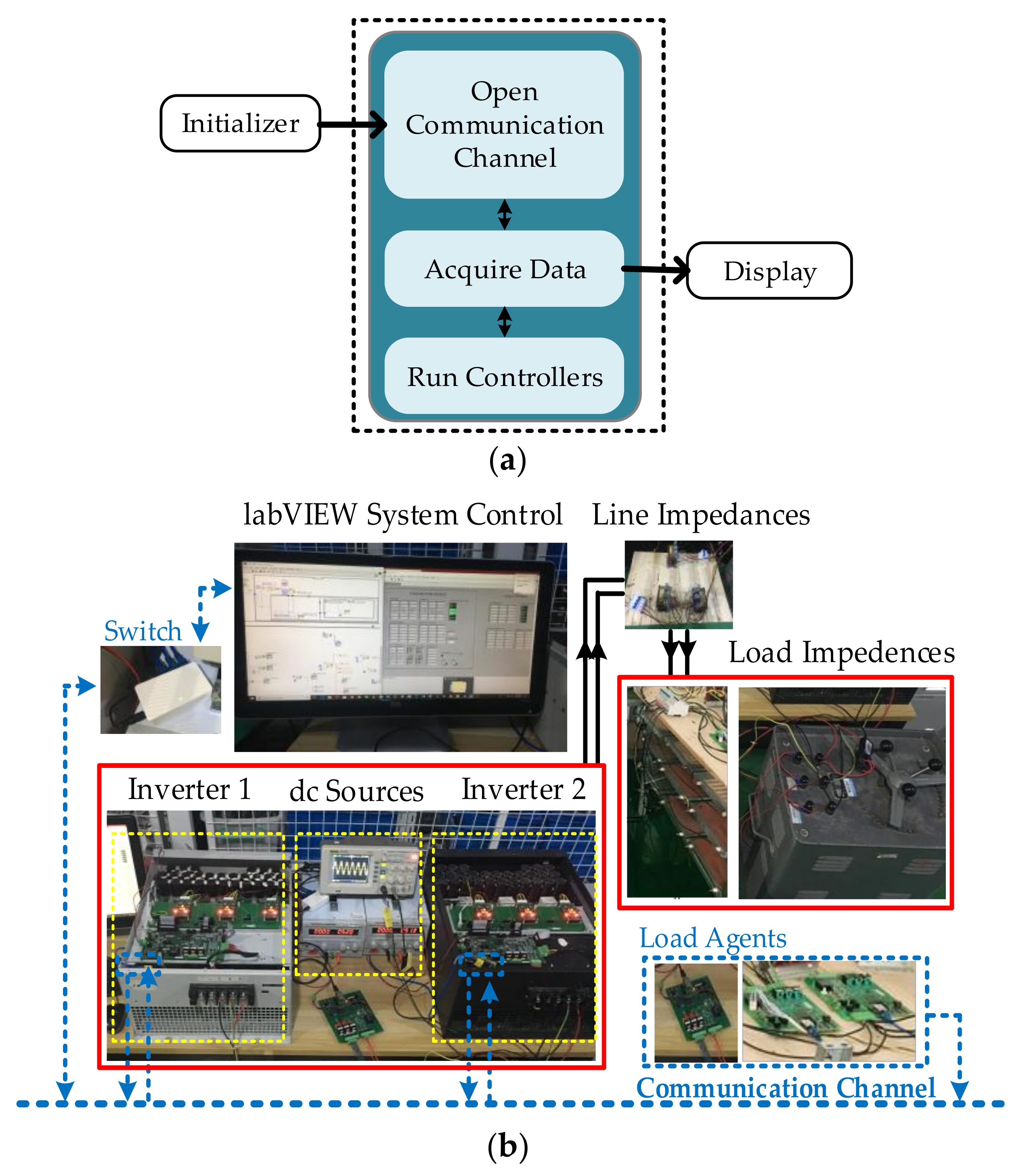
4.3. Experimental Results

An accompanying experiment is carried out to investigate the proposed control scheme. The experiment is conducted for a three-phase, 50-Hz scaled islanded MG prototype, as depicted in Figure 3. The system consists of two identical paralleled DG units with a maximum rating of 3 A, 30 V, connected with RL load via feeder 1 and feeder 2. Ethernet module USR TCP 232 is used for serial communication transmission of data among the data terminal equipment (DTE) and data communication equipment (DCE). The whole platform of islanded MGs is controlled by the desktop control system, wherein LabVIEW has been used to control the DG units.

Figure 8a shows the behavior of load voltage in the presence of disturbance load under a conventional control scheme. Load disturbance of value L_d1 = 1 mH, R_d1 = 5 Ω is added at t₁ as shown in Figure 8b (magnified). From the same figure, 1v load voltage deviation is observed once the disturbance load is added. This deviation is removed when the conventional control strategy is activated at t₂. However, under the conventional control scheme, still, 2.5 V load voltage deviation is observed, as compared to its original state (V_ref = 30 V) as shown in Figure 8c. Figure 8d shows the DGs and load voltage response in the presence of the disturbance load jX_d1/R_d1 under the proposed control scheme. About 0.5 V load voltage deviation is noticed once the disturbance load is exerted at t₁, as shown in Figure 8e (magnified result). This load voltage deviation is removed, and load voltage is restored to its original state (V_ref = 30 V), as shown in Figure 8f (magnified result). System frequency error measured at inverter terminal is regulated within an acceptable range once the proposed control scheme is activated at t₂, as in Figure 8g.

5. Conclusions

In this paper, an enhanced droop control scheme is presented for microgrids working in islanded mode. The control scheme is able to restore the load voltage deviations and fluctuations due to the droop effect and load effect. The proposed study consists of two decoupled methods, the Q-V control layer shares the reactive power proportionally and restores the load voltage magnitudes, while the P-f control layer addresses the active power sharing and frequency stability. Both sets of control layers have been implemented in a distributed manner. At the same time, the distributed secondary layer is used to regulate the system frequency. Mathematical small-signal models were employed to analyze the performance of the presented scheme using pole-zero evolutions with regard to system stability toward variations in control parameters. Various simulations and experimental results, in comparison to the conventional scheme, showed that the proposed methodology is very effective.

References

1. Zurich, C. Power System Models, Objectives and Constraints in Optimal Power Flow Calculations Rainer Bacher; 1993; pp. 217–218. Available online: http://people.ee.ethz.ch/~bacher/publications/thun_paper.pdf (accessed on 18 September 2021).
2. Marcos, F.E.P.; Domingo, C.M.; Roman, T.G.S.; Palmintier, B.; Hodge, B.-M.; Krishnan, V.; García, F.D.C.; Mather, B. A Review of Power Distribution Test Feeders in the United States and the Need for Synthetic Representative Networks. Energies 2017, 10, 1896. [Google Scholar] [CrossRef] [Green Version]
3. Kazmi, S.A.; Shahzad, M.K.; Khan, A.Z.; Shin, D.R. Smart Distribution Networks: A Review of Modern. Energies 2017, 10, 501. [Google Scholar] [CrossRef]
4. El-Khattam, W.; Salama, M. Distributed generation technologies, definitions and benefits. Electr. Power Syst. Res. 2004, 71, 119–128. [Google Scholar] [CrossRef]
5. Ranjan, R.; Das, D. Voltage Stability Analysis of Radial Distribution Networks. Electr. Power Compon. Syst. 2003, 31, 501–511. [Google Scholar] [CrossRef]
6. Bina, M.T.; Kashefi, A. Electrical Power and Energy Systems Three-phase unbalance of distribution systems: Complementary analysis and experimental case study. Int. J. Electr. Power Energy Syst. 2011, 33, 817–826. [Google Scholar] [CrossRef]
7. Bullich-Massagué, E.; Díaz-González, F.; Aragüés-Peñalba, M.; Girbau-Llistuella, F.; Olivella-Rosell, P.; Sumper, A. Microgrid clustering architectures. Appl. Energy 2018, 212, 340–361. [Google Scholar] [CrossRef]
8. The Path of the Smart Grid 18. 2010. Available online: https://ieeexplore.ieee.org/document/5357331 (accessed on 18 September 2021).
9. Habib, S.; Khan, M.M.; Abbas, F.; Ali, A.; Hashmi, K.; Shahid, M.U.; Bo, Q.; Tang, H. Risk Evaluation of Distribution Networks Considering Residential Load Forecasting with Stochastic Modeling of Electric Vehicles. Energy Technol. 2019, 7, 1900191. [Google Scholar] [CrossRef]
10. Nandi, R. Research Papers Impacts of Micro-Grid and dg On Radial. 2019. Available online: https://imanagerpublications.com/article/15500/20 (accessed on 18 September 2021).
11. Han, H.; Hou, X.; Yang, J.; Wu, J.; Su, M.; Guerrero, J. Review of power sharing control strategies for islanding operation of AC microgrids. IEEE Trans. Smart Grid 2016, 7, 200–215. [Google Scholar] [CrossRef] [Green Version]
12. Khan, M.Z.; Khan, M.M.; Xiangming, X.; Khalid, U.; Ahmed, M. An optimal control load demand sharing strategy for multi-feeders in islanded microgrid. Int. J. Adv. Comput. Sci. Appl. 2018, 9, 18–25. [Google Scholar] [CrossRef]
13. Eid, B.M.; Rahim, N.A.; Selvaraj, J.; El Khateb, A.H. Control Methods and Objectives for Electronically Coupled Distributed Energy Resources in Microgrids: A Review. IEEE Syst. J. 2016, 10, 446–458. [Google Scholar] [CrossRef]
14. Han, Y.; Li, H.; Shen, P.; Coelho, E.; Guerrero, J. Review of Active and Reactive Power Sharing Strategies in Hierarchical Controlled Microgrids. IEEE Trans. Power Electron. 2017, 32, 2427–2451. [Google Scholar] [CrossRef] [Green Version]
15. Hashmi, K.; Khan, M.M.; Shahid, M.U.; Nawaz, A.; Khan, A.; Jun, J.; Tang, H. An energy sharing scheme based on distributed average value estimations for islanded AC microgrids. Int. J. Electr. Power Energy Syst. 2020, 116, 105587. [Google Scholar] [CrossRef]
16. Guerrero, J.; Chandorkar, M.; Lee, T.-L.; Loh, P.C. Advanced Control Architectures for Intelligent MicroGrids—Part I: Decentralized and Hierarchical Control. IEEE Trans. Ind. Electron. 2013, 60, 1254–1262. [Google Scholar] [CrossRef] [Green Version]
17. Khan, M.Z.; Khan, M.M.; Jiang, H.; Hashmi, K.; Shahid, M.U. An improved control strategy for three-phase power inverters in islanded ac microgrids. Inventions 2018, 3, 47. [Google Scholar] [CrossRef] [Green Version]
18. Shahid, M.U.; Khan, M.M.; Yuning, J.; Hashmi, K.; Mumtaz, M.A.; Tang, H. An adaptive droop technique for load sharing in islanded DC micro grid with faulty communication. EPE J. 2021, 1–15. [Google Scholar] [CrossRef]
19. Hashmi, K.; Khan, M.M.; Xu, J.; Shahid, M.U.; Habib, S.; Faiz, M.T.; Tang, H. A Quasi-average estimation aided hierarchical control scheme for power electronics-based islanded microgrids. Electronics 2019, 8, 39. [Google Scholar] [CrossRef] [Green Version]
20. Lee, C.T.; Chuang, C.C.; Chu, C.C.; Cheng, P.T. Control Strategies for Distributed Energy Resources Interface Converters in the Low Voltage Microgrid. In Proceedings of the 2009 IEEE Energy Conversion Congress and Exposition, San Jose, CA, USA, 20–24 September 2009; pp. 2022–2029. [Google Scholar]
21. Chandorkar, M.C.; Divan, D.M.; Adapa, R. Control of Parallel Connected Inverters in Standalone ac Supply Systems. IEEE Trans. Ind. Appl. 1993, 29, 136–143. [Google Scholar] [CrossRef]
22. Byun, Y.B.; Koo, T.G.; Joe, K.Y.; Kim, E.S.; Seo, J.I.; Kim, D.H. Parallel Operation of Three-phase UPS Inverters by Wireless Load Sharing Control. In Proceedings of the INTELEC Twenty-Second International Telecommunications Energy Conference (Cat. No.00CH37131), Phoenix, AZ, USA, 10–14 September 2000; pp. 526–532. [Google Scholar]
23. Guerrero, J.; De Vicuña, L.G.; Matas, J.; Miret, J.; Castilla, M. Output impedance design of parallel-connected UPS inverters. IEEE Int. Symp. Ind. Electron. 2004, 2, 1123–1128. [Google Scholar] [CrossRef]
24. Tuladhar, A.; Jin, H.; Unger, T.; Mauch, K. Control of Parallel Inverters in Distributed AC Power Systems with Consideration of Line Impedance Effect. IEEE Trans. Ind. Appl. 2000, 36, 131–138. [Google Scholar] [CrossRef]
25. Salman, H.; Khan, M.M.; Abbas, F.; Ali, A.; Faiz, M.T.; Ehsan, F.; Tang, H. Contemporary trends in power electronics converters for charging solutions of electric vehicles. CSEE J. Power Energy Syst. 2020, 6, 911–929. [Google Scholar] [CrossRef]
26. Pei, Y.; Jiang, G.; Yang, X.; Wang, Z. Auto-Master-Slave Control Technique of Par allel Inverters in Distributed AC Power Systems and UPS. In Proceedings of the 2004 IEEE 35th Annual Power Electronics Specialists Conference (IEEE Cat. No.04CH37551), Aachen, Germany, 20–25 June 2004; pp. 2050–2053. [Google Scholar]
27. Divshali, P.H.; Alimardani, A.; Hosseinian, S.H.; Abedi, M. Decentralized Cooperative Control Strategy of Microsources for Stabilizing Autonomous VSC-based microgrids. IEEE Trans. Power Syst. 2012, 27, 1949–1959. [Google Scholar] [CrossRef]
28. Banda, J.; Siri, K. Improved central-limit control for parallel-operation of DC-DC power converters. In Proceedings of the PESC ’95—Power Electronics Specialist Conference, Atlanta, GA, USA, 18–22 June 1995; pp. 1104–1110. Available online: https://ieeexplore.ieee.org/document/474953/authors#authors (accessed on 18 September 2021).
29. Sun, X.; Lee, Y.-S.; Xu, D. Modeling, Analysis, and Implementation of Parallel Multi-Inverter Systems with Instantaneous. IEEE Trans. Power Electron. 2003, 18, 844–856. [Google Scholar]
30. Yao, W.; Chen, M.; Matas, J.; Guerrero, J.; Qian, Z.-M. Design and analysis of the droop control method for parallel inverters considering the impact of the complex impedance on the power sharing. IEEE Trans. Ind. Electron. 2011, 58, 576–588. [Google Scholar] [CrossRef]
31. Guerrero, J.; Vasquez, J.C.; Matas, J.; de Vicuña, L.G.; Castilla, M. Hierarchical control of droop-controlled AC and DC microgrids—A general approach toward standardization. IEEE Trans. Ind. Electron. 2011, 58, 158–172. [Google Scholar] [CrossRef]
32. He, J.; Li, Y.W.; Guerrero, J.M.; Blaabjerg, F.; Vasquez, J.C. An Islanding Microgrid Power Sharing Approach Using Enhanced Virtual Impedance Control Scheme. IEEE Trans. Power Electron. 2013, 28, 5272–5282. [Google Scholar] [CrossRef]
33. Li, Y.; Li, Y.W. Decoupled Power Control for an Inverter Based Low Voltage Microgrid in Autonomous Operation. In Proceedings of the 2009 IEEE 6th International Power Electronics and Motion Control Conference, Wuhan, China, 17–20 May 2009; Volume 3, pp. 2490–2496. [Google Scholar]
34. Li, Y.; Li, Y.W. Virtual Frequency-Voltage Frame Control of Inverter Based Low Voltage Microgrid. In Proceedings of the 2009 IEEE Electrical Power & Energy Conference (EPEC), Montreal, QC, Canada, 22–23 October 2009; pp. 1–6. [Google Scholar]
35. Li, Y.; Li, Y.W. Power management of inverter interfaced autonomous microgrid based on virtual frequency-voltage frame. IEEE Trans. Smart Grid 2011, 2, 30–40. [Google Scholar] [CrossRef]
36. Perreault, D.; Selders, R.; Kassakian, J. Frequency-Based Current-Sharing Techniques for Paralleled Power Converters. IEEE Trans. Power Electron. 1998, 13, 626–634. [Google Scholar] [CrossRef]
37. He, J.; Li, Y.W. An Enhanced Microgrid Load Demand Sharing Strategy. IEEE Trans. Power Electron. 2012, 27, 3984–3995. [Google Scholar] [CrossRef]
38. Vasquez, J.C.; Guerrero, J.; Luna, A.; Rodriguez, P.; Teodorescu, R. Adaptive Droop Control Applied to Voltage-Source Inverters Operating in Grid-Connected and Islanded Modes. IEEE Trans. Ind. Electron. 2009, 56, 4088–4096. [Google Scholar] [CrossRef]
39. He, J.; Li, Y.W. An accurate reactive power sharing control strategy for DG units in a microgrid. In Proceedings of the 8th International Conference Power Electron—ECCE Asia Green World with Power Electron, ICPE 2011-ECCE Asia, Jeju, Korea, 30 May–3 June 2011; pp. 551–556. [Google Scholar] [CrossRef]
40. Habib, S.; Khan, M.M.; Abbas, F.; Numan, M.; Ali, Y.; Tang, H.; Yan, X. A framework for stochastic estimation of electric vehicle charging behavior for risk assessment of distribution networks. Front. Energy 2019, 14, 298–317. [Google Scholar] [CrossRef]
41. Majumder, R.; Member, S.; Ghosh, A. Angle Droop versus Frequency Droop in a Voltage Source Converter Based Autonomous Microgrid. In Proceedings of the 2009 IEEE Power & Energy Society General Meeting, Calgary, AB, Canada, 26–30 July 2009. [Google Scholar]
42. Majumder, R.; Member, S.; Chaudhuri, B.; Ghosh, A. Improvement of Stability and Load Sharing in an Autonomous Microgrid Using Supplementary Droop Control Loop. IEEE Trans. Power Syst. 2010, 25, 796–808. [Google Scholar] [CrossRef] [Green Version]
43. Guerrero, J.M.; Matas, J.; de Vicuña, L.G.; Castilla, M.; Miret, J. Decentralized Control for Parallel Operation of Distributed Generation Inverters Using Resistive Output Impedance. IEEE Trans. Ind. Electron. 2007, 54, 994–1004. [Google Scholar] [CrossRef]
44. Lee, C.T.; Chu, C.C.; Cheng, P.T. A new droop control method for the autonomous operation of distributed energy resource interface converters. IEEE Trans. Power Electron. 2013, 28, 1980–1993. [Google Scholar] [CrossRef]
45. Bidram, A.; Member, S.; Davoudi, A. Hierarchical Structure of Microgrids Control System. IEEE Trans. Smart Grid 2012, 3, 1963–1976. [Google Scholar] [CrossRef]
46. Arboleya, P.; Diaz, D.; Guerrero, J.M.; Garcia, P.; Briz, F.; Aleixandre, J.G. An improved control scheme based in droop characteristic for microgrid converters. Electr. Power Syst. Res. 2010, 80, 1215–1221. [Google Scholar] [CrossRef]
Figure 1. MG power network model and proposed control strategy.
Energies 14 06092 g001
Figure 2. (a) Power controller of ith inverter (b) inner voltage and current control layer.
Energies 14 06092 g002
Figure 3. (a) General procedure of LabVIEW control system. (b) Laboratory experimental prototype.
Energies 14 06092 g003
Figure 4. Poles zero plots: (a) effect of the mPi variation; (b) effect of the nQi variation; (c) effect of the time delay td on system stability.
Energies 14 06092 g004
Figure 5. MATLAB/Simulink results with the conventional control scheme. (a) Behavior of load voltage and inverter terminal voltage. (b) Disturbance load jXd1/Rd1 added at t1. (c) Voltage regulation with the conventional control scheme. (d) Real and reactive power sharing. (e) Magnified active power. (f) Magnified reactive power.
Energies 14 06092 g005
Figure 6. MATLAB/SIMULINK results with proposed control scheme. (a) Behavior of load voltage and inverter terminal voltages. (b) Disturbance load jXd1/Rd1 added at t1. (c) Voltage regulation with proposed control scheme. (d) Real power sharing. (e,f) Magnified active power. (g) Reactive power sharing. (h) Magnified reactive power.
Energies 14 06092 g006
Figure 7. Frequency (angular) regulation.
Energies 14 06092 g007
Figure 8. Experimental results. (a) Behavior of load voltage and inverter terminal voltages with conventional control scheme. (b) Disturbance load jXd1/Rd1 added at t1. (c) Voltage regulation with conventional control scheme. (d) Behavior of load and inverter terminal voltages with proposed control scheme. (e) Disturbance load jXd1/Rd1 added at t1. (f) Voltage regulation with proposed control scheme. (g) Frequency regulation, (h) Magnified Frequency Regulation Curve.
Energies 14 06092 g008