The Role of Discounting in Energy Policy Investments

Abstract

For informing future energy policy decisions, it is essential to choose the correct social discount rate (SDR) for ex-ante economic evaluations. Generally, costs and benefits—both economic and environmental—are weighted through a single constant discount rate. This leads to excessive discounting of the present value of cash flows progressively more distant over time. Evaluating energy projects through constant discount rates would mean underestimating their environmental externalities. This study intends to characterize environmental–economic discounting models calibrated for energy investments, distinguishing between intra- and inter-generational projects. In both cases, the idea is to use two discounting rates: an economic rate to assess financial components and an ecological rate to weight environmental effects. For intra-generational projects, the dual discount rates are assumed to be constant over time. For inter-generational projects, the model is time-declining to give greater weight to environmental damages and benefits in the long-term. Our discounting approaches are based on Ramsey’s growth model and Gollier’s ecological discounting model; the latter is expressed as a function of an index capable of describing the performance of a country’s energy systems. With regards to the models we propose, the novelty lies in the calibration of the “environmental quality” parameter. Regarding the model for long-term projects, another innovation concerns the analysis of risk components linked to economic variables; the growth rate of consumption is modelled as a stochastic variable. The defined models were implemented to determine discount rates for both Italy and China. In both cases, the estimated discount rates are lower than those suggested by governments. This means that the use of dual discounting approaches can guide policymakers towards sustainable investment in line with UN climate neutrality objectives.

1. Introduction

Nowadays, energy policies are a key governmental instrument for achieving economic, environmental, and social objectives, encouraging sustainable development, providing environmental protection, and containing greenhouse gas emissions (GHG) [1]. In this respect, the path to energy transition—increasingly advocated for by governments—is driven by investment programmes whose effects often manifest themselves in the long term; these include energy infrastructure and the pricing of environmental externalities such as carbon emissions [2]. Thus, choosing more sustainable investments means making intertemporal decisions. Such choices involve trade-offs between benefits and costs that occur at different times [3]. It follows that a critical issue in environmental and resource economics is the choice of social discount rate (SDR), as it significantly influences the outcome of a cost–benefit tests [4,5]. A social discount rate reflects a society’s relative assessment of well-being today versus well-being in the future [6]. The SDR allows the costs and benefits that an investment generates over time to be weighted to make them economically comparable. It is therefore a fundamental parameter for being able to express an opinion on the economic performance of an investment project whenever the analysis is conducted from the point of view of a public operator or of the community [7].

Choosing an appropriate social discount rate is crucial for cost–benefit analysis. Choosing too high a social discount rate could preclude the realization of many desirable public projects for society, in terms of extra-financial repercussions. Conversely, setting an SDR that is too low would risk steering investment decisions towards economically inefficient investments. Furthermore, a relatively high social discount rate ends up giving less weight to the benefit and cost streams that occur in progressively more distant times, favouring projects with benefits that occur at the beginning of the analysis period [8].

The choice of social discount rate affects both the ex-ante decision that allows the testing of whether a specific public sector project deserves funding, and the ex-post evaluation of its performance [9].

The issue of discounting is also crucial for energy efficiency projects. In this case, investors must weight higher initial costs against future energy savings [10]. There are two aspects of energy projects that need to be addressed: Firstly, these are investments that have multiple extra-financial effects on the community, so their effectiveness is more of a social nature rather than a specifically financial one. Secondly, the time perspective is very long for some initiatives [11]; see, among others, the European Green Deal projects, with targets for 2050 [12], or energy transition programmes to curb global warming, whose effects last for centuries [13].

To guide the decision-making process towards efficient investments that respect the defined programmatic guidelines, it is necessary to attribute a greater ‘value’ to the extra-financial effects that the intervention initiatives generate on the community in the analysis. According to Kula and Evans [14], in a moment of strong environmental stress like the one we are experiencing, environmental effects should be discounted separately and differently from economic impacts. In particular, the challenge today is to fix the discount rate for environmental effects at a rate that reaches either a natural capital depletion rate that maximises the utility of consumption of current and future generations, or the preservation of natural capital. One cannot assume a common discount rate for both natural and man-made capital, since natural capital is finite, while man-made capital is unlimited. So, there should be two discount rates. On the contrary, the two discount rates can only coincide if the demand for ecosystem goods and services does not exceed the ecosystem’s regenerative ability.

The aim of this paper is to propose an innovative economic–environmental (or dual) discounting approach in which environmental externalities are weighted at a different and lower rate than that used for strictly financial cash-flows. This is possible because the social welfare function (SWF), from which the social discount rate derives, is no longer only a function of consumption—and therefore of economic parameters—but also of environmental quality. With this research, we want to define a dual discounting specification for energy projects. Specialising the discounting rate according to the investment sector can lead to a fairer and more equitable allocation of resources [11,15]; specifically, to consider the performance of the energy systems of individual countries, the variable “environmental quality” is defined as a function of the Energy Transition Index (ETI) [16].

In addition, we distinguish between intra-generational energy projects (or those with short-term effects) and inter-generational energy projects (or those with long-term effects). In the first case, we define a dual discounting approach based on time-constant environmental and economic discount rates. In the second case, both discount rates—environmental and economic—are based on a time-declining structure. The use of constant discount rates for projects with long-term implications would end up excessively contracting the present value of progressively more distant costs and benefits over time.

This paper is divided into the following four sections: Section Two first proposes a review of the relevant literature. Section Three defines the theoretical framework of the two environmental–economic discounting models. In Section Four, we implement the models defined to estimate constant and declining discount rates, with reference to both the Italian and Chinese economies. Section Five concludes and discusses energy policy implications.

2. Literature Review

The social discount rate (SDR) plays a critical role in cost–benefit analysis (CBA). The SDR allows the comparison of socio-economic costs and benefits—expressed in monetary terms—in order to make a judgement on the efficiency of a project, programme, or policy [17]. This judgement is summarised by performance indicators such as the economic net present value (ENPV). This indicator is a measurement of an investment’s marginal utility for ‘present’ society [18,19]:

$$\mathrm{ENPV}= \frac{B_t-C_t}{{(1+SDR)}^t}$$

(1)

In which B_t and C_t represent, respectively, the benefits and costs arising at time t; 1/(1 + SDR) is the discount factor. (1) shows that as the discount rate increases, the present value of net benefits decreases, as they become more distant from the time of valuation.

The effect of the contraction of the present value of cash flows is a crucial issue when the objects of analysis are long-lived projects, whose effects extend for at least 30–40 years and therefore involve more than one generation [6]. In the valuation of intergenerational projects, such as those with environmental impacts, the choice of appropriate discount rate involves the additional challenge of taking intergenerational equity into account [9,20].

This is one of the main reasons why there is still no consensus on the discount rate to be used in valuations. The issue becomes even more complex when environmental effects make large contributions and mainly occur in the long run.

The literature review shows that the most widely used approach to estimate the discount rate is the social rate of time preference (SRTP) [21,22]. According to this approach, the social welfare function (SWF) depends on the utility U(c) of income or consumption c alone. In the formula:

$$\mathrm{SWF}={{\displaystyle \int }}_{t=0}^{\infty }{U(c}_t{) e}^{-\rho t}dt$$

(2)

SWF is dependent on the following parameters: ${U(c}_t),$ which represents the utility that society derives from public and private per capita consumption at time t; $e^{-\rho t}$ is the discount factor that allows the incremental utility resulting from an additional unit of consumption at time t to be weighted; ρ represents the rate at which future utility is discounted. This last parameter is also called the pure rate of time preference. In order to determine the discount rate that society should apply to incremental consumption, it is first necessary to estimate the discount factor by maximising the SWF. If W denotes the integral of equation 2, then the derivative of W with respect to consumption in period t represents the discount factor and can be interpreted as the social present value of an incremental unit of consumption in period t [21]. The social discount rate is equal to the proportional rate of decrease in this discount factor over time. In other words, this parameter—also called SRTP—is the rate at which the value of a small increment of consumption falls as time changes. It is shown that the SRTP is a function of two components [9]. The first is ρ, the pure time preference rate (or the utility discount rate). ρ reflects the importance that society attaches to the welfare of the current generation relative to the welfare of the future generation. The second contribution is the product of the elasticity of the marginal utility of consumption η and the growth rate of per capita consumption g. This product shows that an additional unit of consumption for a future generation has a lower utility value than an incremental unit of consumption for the current generation [8]. The formula:

SRTP = ρ + η × g

(3)

(3), also known as the Ramsey formula, depends only on economic parameters and is time-constant, i.e., it leads to estimating a constant discount rate throughout the analysis period. Therefore, according to some authors, this approach fails to properly consider environmental externalities, which often occur in the long term. In this regard, Emmerling et al. [23] argue that the climate goals of the Paris Agreement (2015) can only be achieved by employing very low discount rates, such as the one estimated by Stern [24]. Similarly, van den Bijgaart et al. [25] and van der Ploeg and Rezai [26], using analytical integrated assessment models (IAMs), reveal that the discount rate is a key factor in the social cost of carbon. Gollier [27] proposes an extension of the Ramsey formula for projects with long-term effects, e.g., investments for climate change that reduce greenhouse gas emissions. The assumption is that the consumption level in SWF is uncertain and that fluctuations in consumption growth are distributed independently and normally. According to these assumptions, (3) becomes:

$$\mathrm{SRTP}=\rho +\eta \times {\mu }_g-0.5 \times {\eta }^2 \times {\mathsf{\sigma }}_g^2$$

(4)

where μ_g and ${\sigma }_g^2$ are respectively the consumption growth rate mean and variance. 0.5 × η² ×${\sigma }_g^2$ is the precautionary term and indicates the planner’s intention to save more now in favour of future benefits. This term, called “precautionary”, summarizes the uncertainty of the growth rate of consumption and determines a reduction in the value of the discount rate [18,27]. Luo et al. [3] demonstrate that non-diversifiable idiosyncratic risk reduces the discount rate and increases the present value of the uncertain future benefits of projects.

Other scholars suggest the use of dual discounting approaches, whereby environmental components are weighted at a lower “ecological” rate than the “economic” rate, which is useful for assessing strictly financial costs and revenues [14,28,29,30,31]. This means that the economic net present value (ENPV) is given by the sum of two rates:

$$\mathrm{ENPV}={\displaystyle \sum }_{t=0}^n\frac{F_t }{{(1+ r_c)}^t}+{\displaystyle \sum }_{t=0}^n\frac{E_t }{{(1+r_q)}^t}$$

(5)

where: F_t and E_t indicate, respectively, the annual economic cash flows and net environmental benefits at time t; r_c represents the consumption discount rate (or economic discount rate); r_q is the environmental quality discount rate (or more simply environmental discount rate), with r_q < r_c. In other words, the environmental and social damages and benefits generated by the project, after being transformed into monetary terms, are discounted using r_q. While the economic benefits and costs are assessed through the r_c [18,20,27]. The formulas for estimating r_c and r_q are derived in the following section, via Formulas (7) and (8).

Another branch of the literature proposes the use of time-declining discount rates to give more weight to distant project effects than is the case when using time-constant discount rates [32,33,34,35,36]. Two methods are used to estimate the declining discount rate (DDR): The expected net present value approach and the consumption-based approach. For both, the theoretical assumption is to include an uncertainty factor in the time-structure of the discount rate. In the ENPV approach, the same discount rate is modelled as an uncertain parameter, while in the consumption-based approach, the uncertainty concerns the growth rate of consumption which appears in the Ramsey formula.

With reference to the first approach, Weitzman [6] shows that estimating ENPV with an uncertain but constant discount rate is equivalent to computing net present value (NPV) with a certain but decreasing “certainty equivalent” until it reaches the minimum possible value at time t = ∞. Thus, if the discount rate is modelled as a stochastic variable, we can first estimate the certainty equivalent discount factor, then the corresponding certainty equivalent discount rate, understood as the exchange rate of the expected discount factor or rate of progression from t to t + 1.

According to Gollier’s consumption-based approach [18,27,29], the absence of a sufficiently large dataset covering the growth process of the economy in the long run implies that parameters μ and σ of (3) can be treated as uncertain. It is then assumed that the consumption log follows a Brownian motion with trend μ(θ) and volatility σ(θ). These values depend on parameter θ, which is uncertain at time 0. These assumptions allow us to transform (3) into a time-declining function.

Weitzman’s [6,32] findings guided the UK and France to adopt discount rates with a declining structure for projects with long-term consequences [37,38]. The U.S. Environmental Protection Agency [39] has also followed suit.

Finally, recent studies analyse the need to use a specific discount rate for environmental sectors and services. Baumgärtner et al. [31] show that ecosystem services should be discounted at significantly lower rates than those used to weight consumer goods. Vazquez-Lavín et al. [40], with reference to projects aimed at preserving biodiversity in marine protected areas in Chile, estimate a declining SDR for eco-system services. Muñoz-Torrecillas et al. [41] estimate an SDR to be employed in the appraisal of afforestation projects in the United States.

With specific reference to the energy sector, Steinbach and Staniaszek [42], Kubiak [10], and Poudineh and Penyalver [2] offer a review of social discount rates for energy transition policies and their implications for decision-making. Foltyn-Zarychta et al. [11] consider employing a lower discount rate than that suggested by the government, as energy policy planning horizons are generally very long. The US Department of Energy (DOE) evaluates a rate of 3% for energy conservation and RES projects. The estimate is based on long-term Treasury bonds, averaged over a 12-year period [42].

The following

Table 1. Literature review on the social discount rate.

Literature Branch	References
Constant and single discounting	[8,21,43,44,45,46,47,48,49,50]
Declining discounting	[3,4,5,6,7,17,20,32,33,34,35,36,51]
Dual discounting	[14,18,28,30]
Specific discount rate per investment sector/area of intervention	Energy systems [11,42] Application for different investment sectors [15] GHG emissions [23] Ecosystem Services [31,40] Afforestation Projects [41]

summarises the main literature studies concerning approaches to estimating the discount rate.

Considering the framework outlined, this research intends to characterise new approaches for estimating SDR for use in economic evaluations of energy interventions and policies. As the literature review shows, there is a lack of studies proposing both constant and declining dual models specifically for the economic evaluation of energy projects. Thus, building on the existing literature, we define a new discounting model in which environmental quality is described as a function of an energy transition index. Specifically, we define: (i) a constant-dual discounting model for intra-generational energy projects, whose effects can be assessed over a thirty-year period. In this case we define an environmental and an economic discount rate, which are constant over time; (ii) a declining-dual discounting model for inter-generational investments, i.e., those with appreciable effects over the long run. In the second case, however, we define an environmental discount and an economic discount, both with a declining structure over time; this is possible because we take macroeconomic risks into account in the modelling.

3. Modelling the Social Discount Rate for Energy Policies

In this section, we characterise discounting models that can fairly account for the environmental impacts of energy policies, both short- and long-term. Section 3.1 focuses on the model for estimating discount rates for intra-generational energy projects, i.e., investments whose impacts occur over a period of at most thirty years. Section 3.2 defines the discounting model for energy projects with long-term effects for which inter-generational equity issues need to be considered.

Both models are based on the use of discount rates, that are lower for discounting environmental externalities than rates which weight only the strictly economic components. This is because the mathematical structure of the discount rate is a function not only of consumption, but also of environmental quality. The latter is, for the first time, expressed as a function of the Energy Transition Index (ETI), to orient decision-making towards investments increasingly in line with climate neutrality goals.

The model for energy intra-generational projects proposes the use of time-constant rates. This is legitimate as the contraction effects on the present value of cash flows are acceptable for time intervals limited to 20–30 years. Instead, in the case of investments with long-run effects, inter-generational equity issues are addressed by using rates with a declining structure over time. Otherwise, long-term environmental damage and benefits would be underestimated, or not considered at all in the analysis.

3.1. A New Discounting Model for Energy Intra-Generational Projects

Our approach to discount the effects of intra-generational projects in the energy field is based on Ramsey’s growth model [47] and Gollier’s ecological discounting model [29].

Gollier [29,51] proposes discounting the environmental components of investment at a different and lower r_q than the r_c needed to weight the strictly financial effects. To derive useful rates discounting different costs and benefits at different time horizons, it is necessary to consider a representative agent consuming two goods whose availability evolves stochastically over time. This is possible by extending Ramsey’s rule (Equation (3)—taking into account the degree of substitutability between the two goods and the uncertainty surrounding economic and environmental growth. The rate at which environmental impacts should be discounted is in general different from the rate at which monetary benefits should be discounted. It is shown that, under Cobb–Douglas certainty and preferences, the difference between the economic and ecological discount rates is equal to the difference between the economic and ecological growth rates.

More specifically, it is assumed that the utility function U_t also depends on environmental quality $q_t$ as well as consumption $c_t$, i.e., U_t = $U\left(c_t, q_t\right)$. In addition, since the environment tends to deteriorate over time, an incremental improvement in environmental quality will be more valuable to future generations than to current ones. Assuming again that $c_t$ is a partial substitute for environmental quality, economic growth has a positive impact on the ecological discount rate, potentially offsetting the effect of environmental deterioration. If the substitutability is limited, the effect of environmental deterioration dominates economic growth. This leads to a low ecological discount rate that allows environmental assets to be preserved.

Based on the assumptions introduced, the inter-temporal SWF becomes the sum of the utilities derived from both consumption $c_t$ and environmental quality $q_t$:

$$SWF ={{\displaystyle \int }}_{t=0}^{\infty }U\left(c_t, q_t\right)· e^{-\rho t}dt$$

(6)

To derive the economic discount rate and the environmental discount rate, we assume that environmental quality is a deterministic function of economic performance: $q_t$ = f($c_t$). Common sense implies that environmental quality is a decreasing function of GDP per capita, but this is much debated in scientific circles. For this reason, it is permissible to assume the following monotone relationship q_t = c_t^ρ, where ρ can be either positive or negative. If we assume that $q_t$ follows a geometric Brownian motion, we obtain an analytical solution for $r_c$ and $r_{q }$. Without going into the analytical demonstration of the formulae, for which we refer to Gollier [29], it should be noted that deriving $U\left(c_t, q_t\right)$ with respect to consumption $c_t$, we have the function describing the economic discount rate $r_c$:

$$r_c=\rho +\left[{\eta }_1+\delta · \left({\eta }_2-1\right)\right] · \left[g_1-0.5 · (1+{\eta }_1+\delta · \left({\eta }_2-1\right)\right] · {\sigma }_{11}$$

(7)

Deriving U(c_t, q_t) with respect to environmental quality q_t, we obtain the ecological discount rate function $r_{q }$:

$$r_{q }=\rho +\left[\left(\delta ·{ \eta }_2{+\eta }_1- 1\right)\right] · \left[g_1- 0.5 · \left(\delta ·{ \eta }_2{+\eta }_1\right)\right] ·{ \sigma }_{11}$$

(8)

(7) and (8) show how r_c and r_q depend on: (i) socio-economic parameters, such as the time preference rate ρ, risk aversion to income inequality η₁, the growth rate of consumption g₁, the uncertainty of the consumption growth rate σ₁₁ in terms of the mean square deviation of the variable; (ii) environmental variables, such as the degree of environmental risk aversion η₂ and the elasticity δ of environmental quality to changes in the growth rate of consumption g₁. The estimation of each parameter is detailed at the end of this section.

The aim of this research is to propose discount rates that adequately account for the costs and benefits of energy investments. The main novelty of the model is therefore the modelling of environmental quality q_t, which for the first time is defined as a function of the Energy Transition Index (ETI). The index, estimated by the World Economic Forum (WEF), provides a framework to compare and support countries in their energy transition needs, considering their current energy system performance and the readiness of their macroeconomic, social, and regulatory environment for transition. The index, which summarises 40 different indicators, is currently available for 114 countries. The scores show that while 92 countries have risen their score over the last 10 years, only 10% of countries have been able to reach consistent gains, which are necessary to achieve climate targets for the next decade.

According to the World Economic Forum report ‘Fostering Effective Energy Transition [16], even as countries continue in their progress in clean energy transition, it becomes necessary to embed the transition in economic, political, and social practices to ensure irreversible progress. For this reason, it is essential to introduce a variable into the mathematical structure of the discount rates that sees the progress of countries on the path to energy transition. This introduces an acceptance criterion that can guide decision-making towards those projects that are in keeping with climate neutrality goals to be achieved by 2030 and 2050.

Defining q_t = f(ETI), we can derive the value of the elasticity δ of environmental quality to changes in the growth rate of consumption as follows. Let c₁ be the GDP per capita of a country and c₂ the relative ETI. The slope of the regression line that correlates the two parameters GDP per capita and ETI corresponds to the value of δ. It follows that a different definition of environmental quality may allow the model to be adapted to the assessment of project categories other than energy projects.

In the following, the approaches to estimate the parameters that make up (7) and (8) are defined.

With reference to socio-economic variables, the time preference rate ρ is the sum of (i) l, which coincides with the average mortality rate for a country—this is because individuals tend to discount future utility according to the probability of being alive at the time of the decision; and (ii) r, or the pure time preference rate. This parameter reflects the irrational behaviour of individuals in making choices about the distribution of resources over time and is generally between 0 and 0.5% [49,50].

The elasticity η₁ of the marginal utility of consumption represents the percentage change in marginal utility resulting from a unit change in consumption [51]. It is a measure of risk aversion to income inequality, and it is estimated using the formula proposed by both Stern [52] and Cowell et al. [53]:

$${\eta }_1=\frac{\log (1 - \mathrm{t})}{\log (1 - \frac{\mathrm{T}}{\mathrm{Y}}) }$$

(9)

(9) is a function of t, the marginal tax rate, and T/Y, the average tax rate.

The growth rate of consumption g₁ expresses the degree of wealth in society and it is generally at the average growth rate of a country’s GDP per capita [46,48].

Finally, a further environmental parameter is η₂, which represents the degree of environmental risk aversion. It can be expressed as a function of the consumption expenditure η* to be allocated to environmental quality, considering that 10% < η * < 50% [29,54,55]:

$${\eta }^{*}=\frac{{\eta }_2 - 1}{{\eta }_1{ + \eta }_2 - 2}$$

(10)

3.2. A New Discounting Model for Energy Inter-Generational Projects

To provide the “right” weighting for the environmental effects of energy projects and policies in the long run, a dual and diminishing discounting approach is proposed. In other words, the structure of the two functions of the discount rate, economic and environmental, defined in the previous section begins decreasing over time.

This can be done by considering macroeconomic risk, i.e., we assume that the growth rate of consumption g₁ is a risky variable. To do this, we must first analyse the variable’s trend over time, then define the probability distribution that best approximates the historical data. From the probability distribution of g₁ thus obtained, we derive the probability distributions of the unknowns r_c and r_q. From these parameters we then derive the values of the economic and environmental discount rates for each of the n years of the analysis period.

The next step is to move from the two uncertain and constant discount rates r_c and r_q, which coincide with the expected value of the probability distributions obtained, to certain but decreasing rates with a ‘certainty equivalent’. This is possible by using the expected net present value (ENPV) approach, according to which, assessing the ENPV with an uncertain but constant discount rate is correspondent to evaluating the NPV with a certain rate, but diminishing with a ‘certainty equivalent’ until it has the minimum value at time t = ∞ [33]. In order to move from the uncertain and constant discount rate to the certain but decreasing discount rate with a ‘certainty equivalent’, it is first necessary to assess the economic discount factors E_c(P_t) and environmental discount factors E_q(P_t), and then r_ct and r_qt:

$$r_{ct} =\frac{ E_c\left(P_t\right)}{ E_c\left(P_t+1\right)}-1$$

(11)

$${ r}_{\mathit{qt}}=\frac{{ E}_q\left(P_t\right)}{{ E}_q\left(P_t+1\right)} - 1$$

(12)

In (11) E_c(P_t) is calculated using the following formula:

$$E_c\left(P_t\right){=E}_c\left[{\displaystyle \sum }_{i=1}^m{p}_{\mathit{rci}}{· e}^{{(-r}_{\mathit{ci}} t)}\right]$$

(13)

where r_ci is the value of the i-th economic discount rate, resulting from the probability distribution of r_c; p_ci = probability of the i-th value of r_c; m = intervals of discretization of probability distributions r_c and r_q;

In (12) E_q(P_t):

$$E_q\left(P_t\right){=E}_q\left[{\displaystyle \sum }_{i=1}^m{p}_{\mathit{rqi}}{· e}^{{(-r}_{\mathit{qi}} t)}\right]$$

(14)

In which r_qi is the value of the i-th environmental discount rate, deriving from the probability distribution of r_q; p_qi = probability of the i-th value of r_q.

4. Application: Estimation of SDRs for Italy and China

The approaches described in Section 3.1 and Section 3.2 are implemented below to estimate discount rates for intra- and inter-generational energy projects for two very different economies: Italy and China. This is to demonstrate how: (i) the model can be applied to any territorial context; (ii) different social, economic, and environmental conditions lead to significantly dissimilar results.

4.1. Estimation of Constant and Dual Discount Rates for Italy and China

In the following we detail the estimation of the socio-economic and environmental parameters in (7) and (8).

The time preference rate ρ is a function of the mortality-based discount rate l and the pure time preference rate r. The first parameter, l, corresponds with the time-averaged mortality rate of the country. Since this rate undergoes small variations over time, it is considered correct to consider data from the last 30 years. l is estimated using mortality rates for the period 1991–2020 given by ISTAT for Italy and by the World Bank for China.

Table 2. Mortality rates for Italy and China over the 30-year period 1991–2020.

Year	1991	1992	1993	1994	1995	1996	1997	1998	1999	2000	Decade average rate
Death rate Italy (%)	0.97	0.96	0.97	0.97	0.98	0.97	0.98	1.00	0.98	0.98	0.98
Death rate China (%)	0.67	0.66	0.66	0.64	0.66	0.66	0.65	0.65	0.65	0.65	0.66
Year	2001	2002	2003	2004	2005	2006	2007	2008	2009	2010	Decade average rate
Death rate Italy (%)	0.96	0.98	1.02	0.95	0.98	0.96	0.98	0.99	1.00	0.99	0.98
Death rate China (%)	0.64	0.64	0.64	0.64	0.65	0.68	0.69	0.71	0.71	0.67	0.67
Year	2011	2012	2013	2014	2015	2016	2017	2018	2019	2020	Decade average rate
Death rate Italy (%)	1.00	1.03	1.00	0.98	1.07	1.00	1.04	1.05	1.05	1.06	1.03
Death rate China (%)	0.71	0.72	0.72	0.72	0.71	0.71	0.71	0.71	0.73	0.74	0.62
Thirty-year average rate Italy (%)											1.00
Thirty-year average rate China (%)											0.68

below shows the result of the calculations.

The result for Italy is l = 1.00%, in line with the estimations obtained by Percoco [46] and Florio and Sirtori [48]. For China l = 0.68%. This lower value compared to Italy is the effect of lower mortality rates over the 30-year period.

The pure time preference rate r is positive and reflects the irrational behaviour of individuals in making choices about the distribution of resources over time. As suggested by both Pearce and Ulph [49] and Evans and Kula [50], 0 < r < 0.5% and is assumed to be 0.3%. It follows that:

$${\rho }_{\mathit{Italy}}=1.00\%+0.3\%=1.30\%;$$

$${\rho }_{\mathit{China}}=0.68\%+0.3\%=0.98\%.$$

By implementing (9) we calculate the elasticity η₁ of the marginal utility of consumption. Using the data of the marginal t and average T/Y individual income tax rates given by the Organization for Economic Cooperation and Development Countries (OECD), we assess log(1 − t), log(1 − T/Y), and the corresponding ratio. Processing returns a value of η₁ = 1.34 for Italy.

The analysis of average and marginal tax rates by income bracket in China gives instead a value of η₁ = 1.14 (source: https://taxsummaries.pwc.com/peoples-republic-of-china/individual/taxes-on-personal-income, 10 July 2021).

In summary, the estimations return the following values:

$${\eta }_1{}_{\mathit{Italy}}=1.34;$$

$${\eta }_1{}_{\mathit{China}}=1.14.$$

Estimates are consistent with known values from the literature, where the social values approach leads to 1 < η < 2.

From the analysis of the trend of per capita GDP growth rate of the two countries, g₁ is estimated for Italy by averaging data over the last forty years, while for China the evaluation is carried out based on data over the last sixty years.

As for the estimation of the two environmental parameters, the value of η₂ is derived from (10), assuming η * = 30%, according to Hoel and Sterner [54], Sterner and Persson [55], and Gollier [29]. Hence, it follows that:

$${\eta }_2{}_{\mathit{Italy}}=1.15;$$

$${\eta }_2{}_{\mathit{China}}=1.06.$$

δ expresses the sensitivity of environmental quality q, expressed through the ETI, to changes in consumption c. The latter parameter is related to GDP per capita. For 115 countries, the index values in 2021 are related to their GDP per capita in the same year. Figure 1 gives the results of the ETI-GDP per capita regression analysis, from which δ is 0.23.

Table 3. Estimation of r_C and r_q for Italy and China.

Parameter	Value for Italy	Value for China
l	1.00%	0.68%
r	0.30%	0.30%
ρ	1.30%	0.98%
η1	1.34	1.14
g1	1.22%	8.17%
η2	1.15	1.06
σ11	0.03%	0.46%
δ	0.23	0.23
rC	2.7%	9.8%
rq	1.8%	4.02%

gives the values obtained for each parameter as well as the estimated r_c and r_q for Italy and China.

4.2. Estimation of Declining and Dual Discount Rates for Italy and China

To estimate time-declining r_ct and r_qt discount rates for energy projects with inter-generational effects, the reference is the approach defined in Section 3.2. Also, in this case, estimations are carried out with reference to both the Italian and Chinese economies.

g_t is estimated based on the growth rate of GDP per capita, in accordance with literature data [46]. As anticipated in Section 4.1, we consider it consistent to select data for the last forty years, i.e., from 1981 to 2020.

In fact, the data reported for the previous period reflect historical and economic contexts that can no longer be linked to either the current or foreseeable future economic, social, and cultural context of the country.

We identify the probability distribution that most closely approximates the historical series to predict the values to be associated with the growth rate of consumption, which in this context is the Weibull curve, chosen based on the Anderson–Darling test. Then, the expected values of the GDP growth rate are predicted by implementing the Monte Carlo analysis, calibrated on 10,000 random trials. The simulation was carried out using Oracle Crystal Ball software. Once the probability distribution of the consumption growth rate g₁ is defined, the probability distributions of the economic discount rate r_c and the ecological discount rate r_q are extracted by implementing (7) and (8).

Table 4. Statistical indices on g₁, r_c, and r_q for Italy.

	Hypothesis: g1	Forecast: rc	Forecast: rq
Trials number	10,000	10,000	10,000
Base case	1.17%	2.66%	1.79%
Mean	1.21%	2.71%	1.81%
Median	1.49%	3.09%	1.98%
Standard deviation	1.69%	2.33%	1.02%
Variance	0.03%	0.05%	0.01%
Kurtosis	4.75	4.75	4.75
Variation coefficient	1.40	0.86	0.56
Min	−8.56%	−10.71%	−4.08%
Max	4.82%	7.67%	3.99%
Mean standard error	0.02%	0.02%	0.01%

shows the values of the statistical indices for the Monte Carlo simulation. The calculations indicate that: g₁ has values between −8.56% and 4.82%, and after 10,000 simulations the standard error of the mean is 0.02%; r_c and r_q have values between −10.71%–7.67% and −4.08%–3.99% respectively. In both cases, the mean standard error is acceptable as it is 0.02% and 0.01% respectively after 10,000 trials. Since negative discount rates have no economic significance, only positive values are considered in the definition of the declining structure of the two rates.

The analysis interval chosen for China is that between 1960–2020, in which the GDP growth trend rate tends to be steadily increasing. In this case, the Anderson–Darling test showed that the curve that best approximates the historical data is the logistic curve.

Again, the likely values of the GDP growth rate are predicted by implementing the Monte Carlo analysis, based on 10,000 random trials.

Table 5. Statistical indices on g₁, r_c and r_q for China.

	Hypothesis: g1	Forecast: rc	Forecast: rq
Trials number	10,000	10,000	10,000
Base case	8.17%	9.86%	4.02%
Mean	8.79%	10.57%	4.262%
Median	8.81%	10.60%	4.272%
Standard deviation	5.62%	6.51%	2.18%
Variance	0.32%	0.42%	0.047%
Kurtosis	4.26	4.26	4.26
Variation coefficient	0.6399	0.6157	0.5714
Min	−18.96%	−21.55%	−6.49%
Max	40.58%	47.38%	16.58%
Mean standard error	0.06%	0.07%	0.022%

shows the values of the statistical indices for the forecast: g₁ has values between −18.96% and 40.58%, and after 10,000 simulations, the standard error of the mean is 0.06%. Furthermore, in the case of the simulations of r_c and r_q, the standard error is acceptable because it holds for the first variable at 0.07% and for the second at 0.02%. In addition, only positive values for the two discount rates are considered. This assumption is acceptable because the probability of having a positive discount rate r_c is 95.06% and the probability that the discount rate r_q is greater than 0 is 95.96%.

The probability distributions of r_c and r_q obtained are first discretized into 100 intervals. Then, for each of the two distributions, we estimate the probability that the average rate of each interval has of occurring. Given the set of values to be associated with the discount rates r_c and r_q and their probability, the equivalent certainty discount factors E_c(P_t) and E_q(P_t) are estimated using formulae (11) and (12). Finally, using (13) and (14) for each instant t leads to the estimation of the time sequence of the declining economic discount rate r_ct and the declining ecological discount rate r_qt. These are declining functions along the time horizon, assumed to be 300 years.

Figure 2 and Figure 3 illustrate the term-structure of the economic and environmental discount rates for Italy and China respectively.

5. Results and Discussion

As Table 3 indicates, the values of the discount rates to be used in the analysis of intra-generational energy projects for Italy are significantly lower than those obtained for China. In fact, r_c and r_q for Italy are 2.7% and 1.8% respectively, while for China r_c is 9.8% and r_q is 4.0%. It should be noted that the difference between the environmental and economic discount rates for China is marked. On the contrary, in the Italian case, the values of the two discount rates are much closer to each other.

The implementation of the discounting model for energy inter-generational projects leads to the following results. For Italy:

• The economic discount rate function r_ct for Italy begins from an initial value of 3.4% to attain a value of 0.7% after 300 years, thus decreasing by about 2.6%.
• The environmental discount rate r_qt, on the other hand, takes on significantly smaller values of r_ct, starting from 1.92% and reaching 0.18% after 300 years.
• The average economic discount rate for the first 30 years is about 3.0%, which coincides with the value of the discount rate suggested by the European Commission [56].
• The average environmental discount rate for the first 20 years is 1.8%, highlighting how from the beginning of the assessment more weight is given to the damages and benefits that the investment generates on the environment.

For China:

• The economic discount rate function r_ct is of 12.90% and reaches a value of 5.36% after 300 years.
• The environmental discount rate r_qt is well below the values of r_ct, as it has an initial value of 4.54% and a final value at t = 300 years of 1.01%.
• The average economic discount rate for the first 30 years is about 10.2%, which is slightly higher than the value of the discount rate suggested by the Asian Development Bank [57] for economic analysis, which is 9.0%.
• The average environmental discount rate for the first 30 years is 4.0%.

Figure 4 and Figure 5 explain the step functions (with solid lines) that approximate the functions (dashed lines) of the economic declining rate and the ecological declining rate for Italy. For practical purposes, it is useful to approximate the declining function to a step function. In other words, it may be permissible to use the same value of the discount rate for a period of thirty years in the analysis. In this time interval, the effect of present value contraction on cash flows can be considered acceptable [37,38,39]. Figure 6 and Figure 7 indicate the same step functions of r_ct and r_qt for China.

The results indicate that the use of two different rates for discounting strictly financial and extra-financial components would allow greater weight to be given to environmental damages and benefits, thus orienting the decision-making process towards more sustainable investment choices.

It is interesting to underline that the two functions of the discount rate for China start from higher initial values than for Italy but decline much more rapidly after the early years of the period of analysis. The higher initial value is mainly due to the higher values of GDP growth rate for China compared to Italy. However, the faster decline in the term-structures of the discount rates is linked to China’s ‘worse’ environmental condition. Indeed, as shown by the lower Energy Transition Index (ETI) value, more weight should be given to environmental impacts of energy projects in China from the early years of the assessment. This is to prioritise investment choices in line with sustainability and climate neutrality objectives to be achieved in the coming decades.

6. Conclusions

Energy transition policies aim to respond to both economic, social, and environmental challenges. Therefore, it is essential to steer the decision-making process towards policy initiatives that ensure a balance between socio-economic benefits and costs. In this context, the choice of discount rate becomes central to comparing policy strategies and investment programmes—but also to determine the speed with which an energy transition policy should be delivered to reach decarbonisation targets within the defined timeframe [2].

Thus, the discount rate affects the final judgement on the efficiency of the investment policy or project. However, there is still no unanimity in the literature as to what value of the discount rate should be used in analyses, or how it should be estimated. The question becomes even more controversial when a very long-term perspective is adopted.

With this research, we propose an innovative discounting approach for discounting energy investments, distinguishing between intra-generational and inter-generational projects.

In the first case, a constant and dual discounting approach is characterised. The discount rate used to discount the environmental components is lower than the discount rate used to weight the strictly financial contributions. However, since the effects of these projects are felt over a period of thirty years at the most, both discount rates are assumed to be time-constant.

For projects with inter-generational environmental effects, a dual and time-declining econometric model is defined to give greater weight to long-term environmental components that would be underestimated using constant rates.

For both models, the main change is that environmental quality is defined as a function of the Energy Transition Index (ETI). It is considered essential to introduce into the mathematical structure of the SDR a variable that considers the progress of countries on the path towards energy transition. In other words, a discount rate defined in this way allows decision makers to be oriented towards those projects that are in line with 2030 and 2050 climate neutrality goals. In addition, the dual and declining approach also takes macroeconomic risk into account, as the growth rate of consumption is modelled as a stochastic variable.

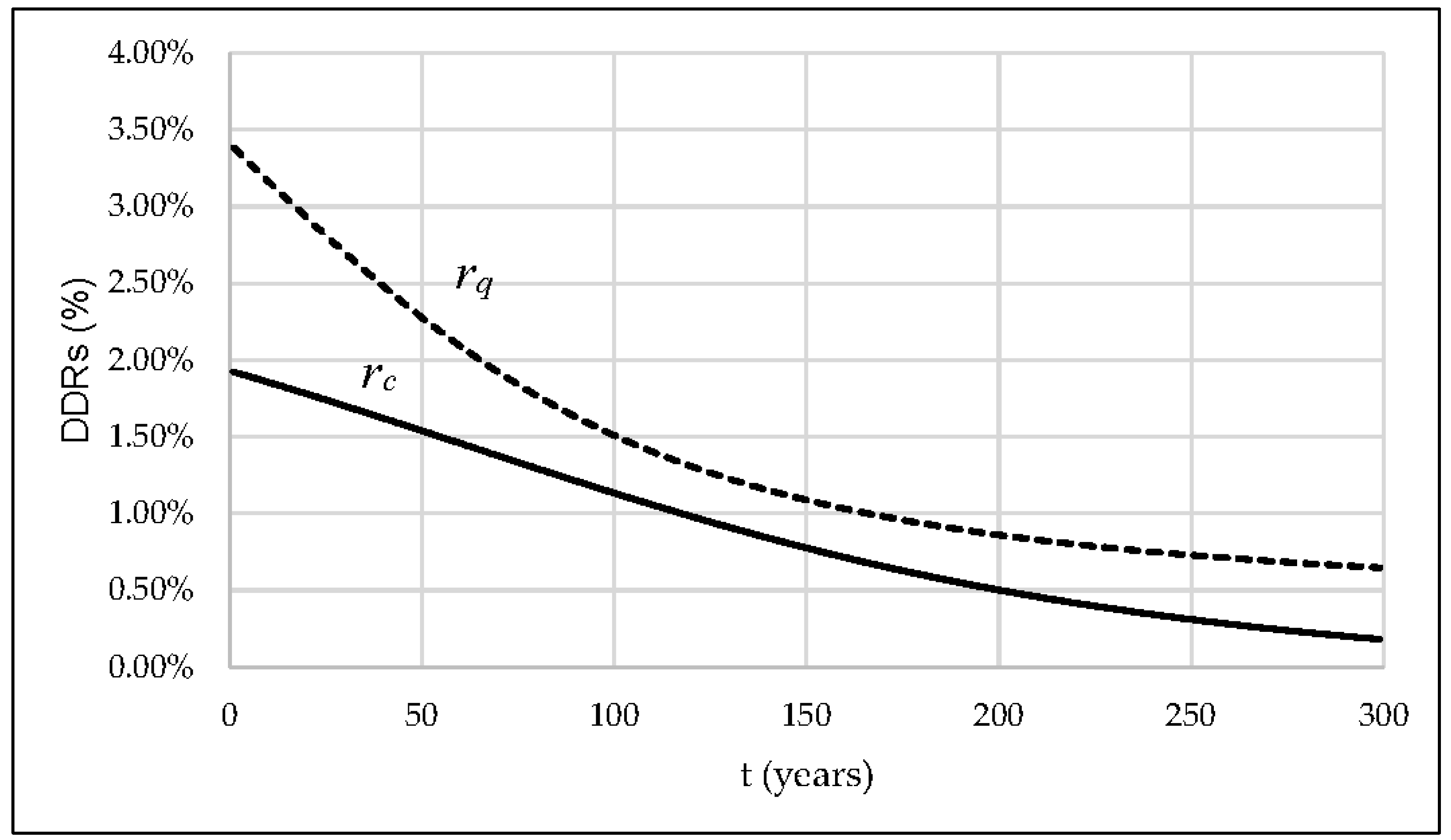
The defined models were implemented to estimate discount rates for both Italy and China. The results obtained show that: (i) in the case of the dual and constant approach for both Italy and China, the environmental discount rate has smaller values than the economic discount rate; (ii) in the case of the dual and declining approach, the two functions of the discount rate—economic and environmental—for China start from higher initial values than for Italy, but decline much faster from the beginning of the analysis period. The higher initial value is mainly due to the higher values of GDP growth rate for China compared to Italy. However, the application demonstrates how China’s ‘worse’ environmental condition leads to a more rapid decline in the term-structures of the discount rates.

While the model is relatively easy to implement, for some countries it may be difficult to find the data needed to estimate each parameter of the model. In addition, estimates of discount rates need to be periodically updated. The application shows, firstly, how different discount rates can be in relation to socio-economic context. Secondly, it is clear how the use of estimated discount rates can favour more sustainable investment choices in line with UN climate neutrality objectives. The decision-making effects on energy policy investments are therefore evident and extremely important; evaluating the economic feasibility of energy projects using dual, and possibly even time-declining approaches, means attributing greater weight to extra-financial damages and benefits. On the contrary, by using the social discount rates provided by governments, which are generally unique and constant over time, policymakers would orient their choices towards investments with higher initial financial returns, without considering the short and long-term repercussions on the environment.

Finally, research perspectives may include the implementation of the model for other countries in order to provide a larger database of environmental and economic discount rates, as well as the adaptation of the model to other sectors of intervention.