Impact of Control Loops on the Passivity Properties of Grid-Forming Converters with Fault-Ride through Capability ^†

Abstract

Due to the increasing integration of renewable energy sources (RES) and a corresponding reduction of conventional generating units, there is nowadays a demand from the power-electronic converters to provide grid-forming properties through proper control of the converter systems. This paper aims to evaluate the impact of various control loops in a grid-forming control strategy equipped with a fault-ride through capability on the passivity properties of the converter system. Through the analysis of the frequency-dependent input admittance of the converter, the main factors affecting the passivity properties are identified. A simplified analytical model is derived in order to propose possible control modifications to enhance the system’s passivity at various frequencies of interest and the findings are validated through detailed time-domain simulations and experimental tests.

1. Introduction

In line with the level of renewable energy sources (RES) replacing conventional generation in the power system, the number of power electronic converters employed for energy conversion is continuously increasing. As a result, selected converter systems interfacing the RES to the power system are required to provide some functionalities to account for the reduction of the conventional generation system. In this regard, grid-forming converter control strategies with a focus on implementing functionalities such as inertia and frequency support, black-start, and synchronization capabilities have been attracting attention in the literature in recent years [1,2,3,4]. In order to provide fault-ride through capability, some of the control strategies are also equipped with a current control structure [3,5]. Nevertheless, non-passive behavior for the grid-forming converter systems that could lead to resonance interactions exists at both low- and high-frequency intervals [6,7,8,9].

Examples of resonance interactions due to the existence of non-passive behavior in the converter systems have been discussed in the literature [10,11,12,13,14,15,16]. In these works, valuable control solutions are investigated in order to guarantee that the energy associated with the resonance condition is dissipated in the converter at the specific frequency of interest. While these findings consider a conventional grid-following control structure that consists of an inner vector current controller together with outer-loop power/voltage controllers and a phase-locked loop (PLL), similarly detailed characterization for grid-forming control structures and a corresponding control parameter tuning to improve passivity is missing and this is addressed in this work.

In this paper, the impact of operating points and different control loops on the passivity properties of a generic converter system with a grid-forming control strategy with fault-ride through capability are investigated. For this purpose, the input admittance of the converter system is derived first. The main contributing factors on the passivity property are identified and recommendations to enhance the system stability through control parameter tuning are proposed. Finally, the analytical findings are verified through detailed time-domain simulations and experimental tests.

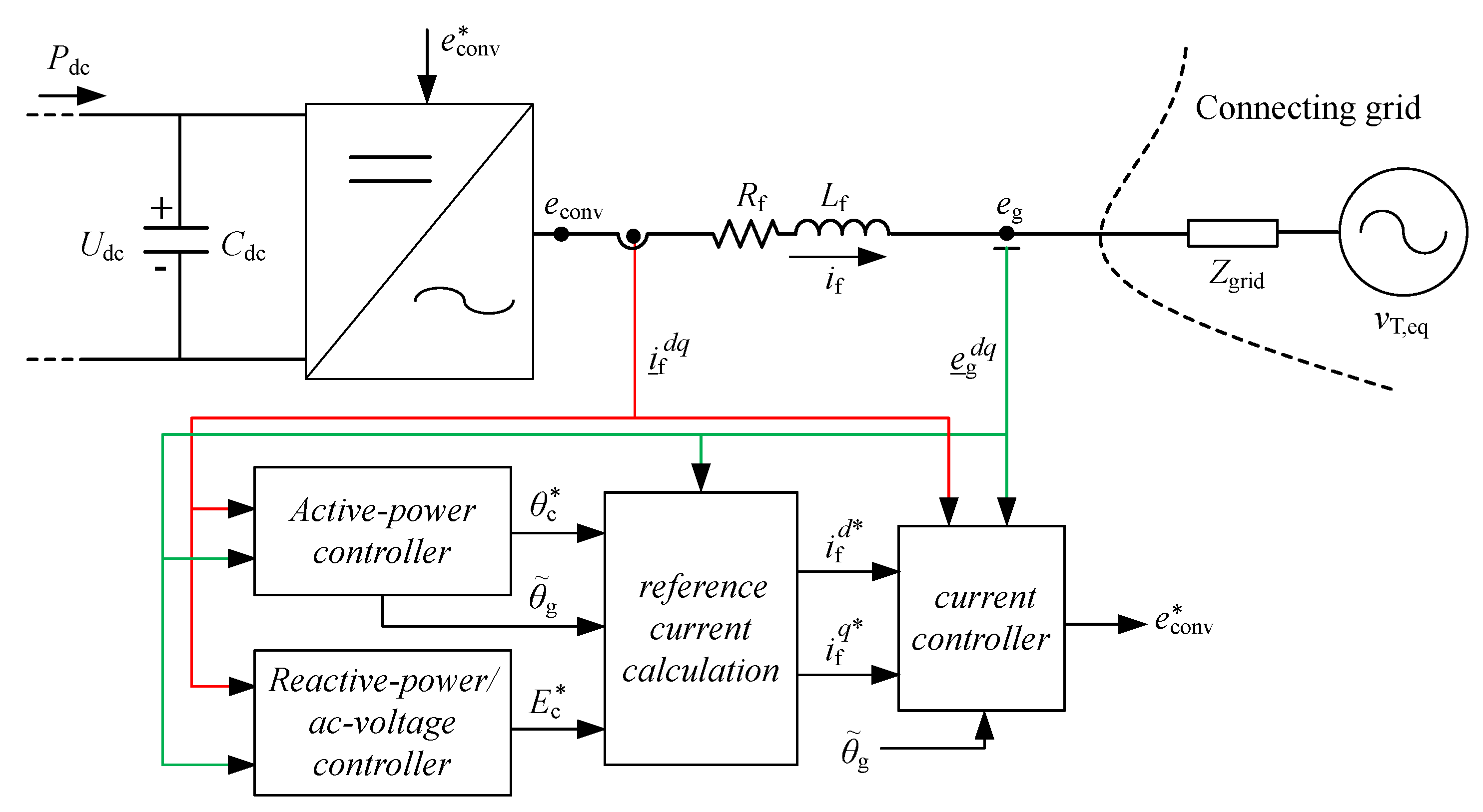
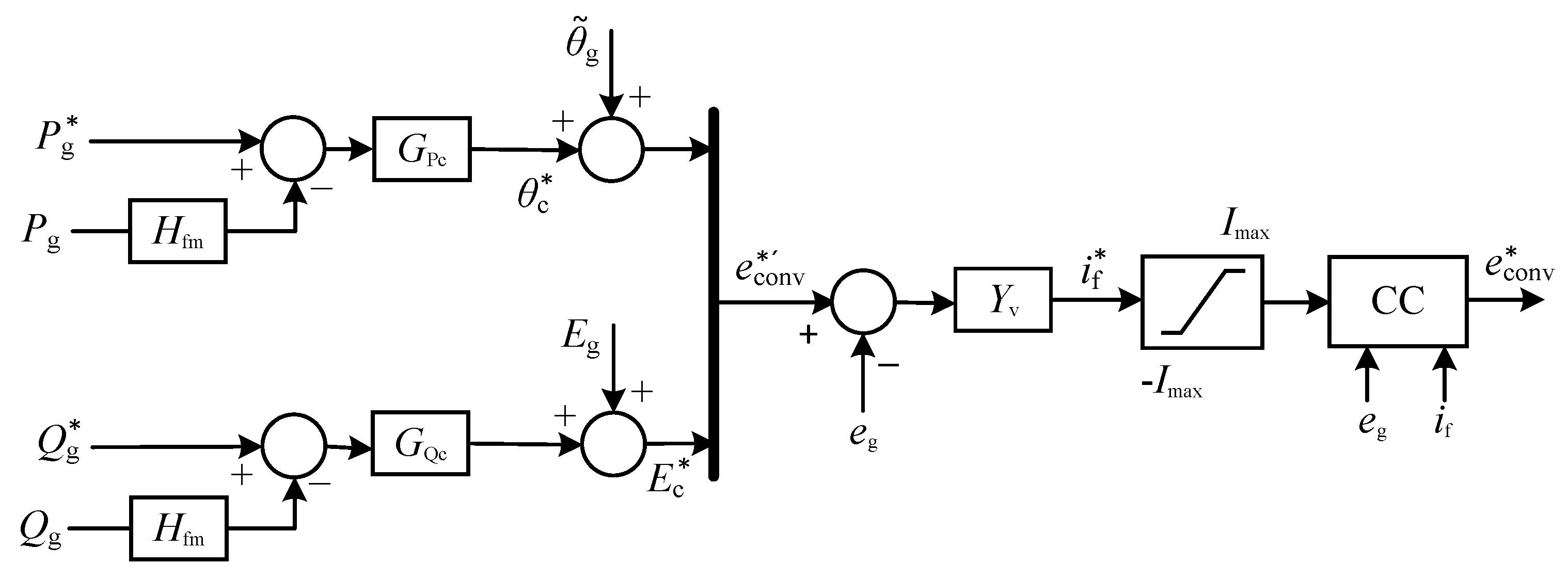
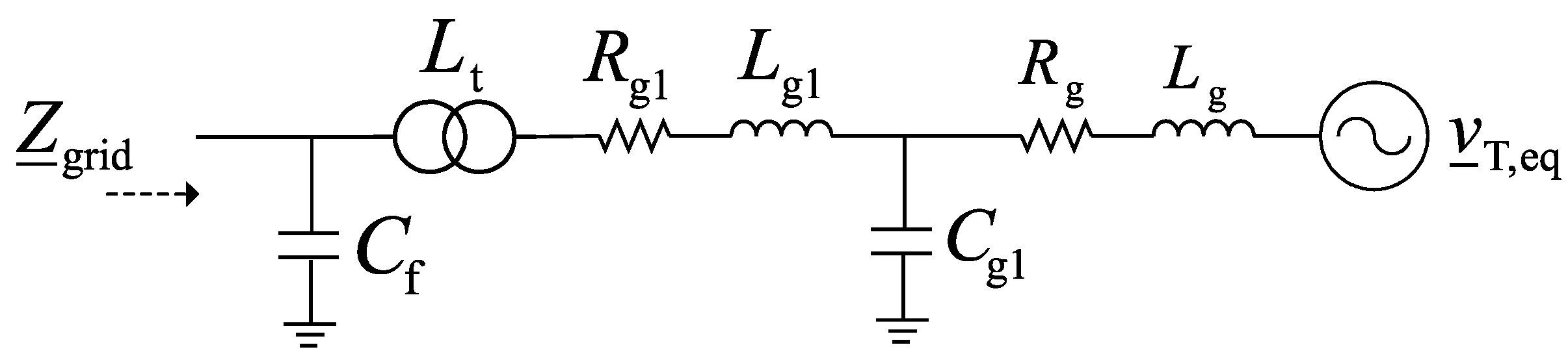
2. System Representation

The investigated system represents a generic converter connected to an ac grid. The converters can resemble, for example, the grid-side of a wind-turbine system, an HVDC, or a STATCOM. The main idea of this work is the investigation of the impact of various control loops on the passivity behavior of power electronic converters interfacing a grid, a simplified generic representation as in Figure 1 is used, where the block scheme of the control approach as well as the equivalent model of the connecting grid is shown. In the figure, $v_{\mathrm{T},\mathrm{eq}}$ and $Z_{\mathrm{grid}}$ denote the voltage source and impedance (including the shunt filter and transformer from the converter) of the Thevenin’s equivalent representation of the rest of the system, respectively. Note that the model in Figure 1 can be used to represent a generic converter system interfaced with the grid by implementing the corresponding control for the converter and the equivalent impedance for the connecting grid.

Figure 1. Schematic of the equivalent circuit of a generic converter system connected to a grid through a phase reactor and possible control blocks.

3. System Modeling and Input-Admittance Derivation

Considering the generic grid-connected converter system in Figure 1 where the detail of the control structure of the converter as described in Figure 2, the input-admittance model is derived in this section. In this setup, the grid voltage is denoted by $e_{\mathrm{g}}$ and the phase reactor is represented with an inductance $L_{\mathrm{f}}$ and resistance $R_{\mathrm{f}}$. The voltage at the converter’s terminals is denoted by $e_{\mathrm{conv}}$, while $i_{\mathrm{f}}$ is the current exchanged between the converter and the grid. Using the estimated grid-voltage angle, ${\tilde{\theta }}_{\mathrm{g}}$ obtained by integrating the estimated grid-frequency (the nominal grid-frequency, ${\omega }_1$ is used for this work as the estimated frequency for simplicity), for coordinate transformation, the current dynamics in the rotating $dq$-frame (with a power invariant transformation) are given by (s is a Laplace transform variable)

$${\underline{e}}_{\mathrm{conv}}^{dq}={\underline{e}}_{\mathrm{g}}^{dq}+j{\omega }_1{L}_{\mathrm{f}}{\underline{i}}_{\mathrm{f}}^{dq}+R_{\mathrm{f}}{\underline{i}}_{\mathrm{f}}^{dq}+s{L}_{\mathrm{f}}{\underline{i}}_{\mathrm{f}}^{dq}$$

(1)

Figure 2. Block diagram of the implemented grid-forming control.

For a typical grid-forming control strategy, the converter reference voltage magnitude ($E_{\mathrm{c}}^{*}$) and load angle (${\theta }_{\mathrm{c}}^{*}$) are in general generated from the reactive-power (or alternatively ac-voltage) and the active-power controllers (see Figure 1 and Figure 2), respectively, as

$$\begin{array}{ccc}{E}_{\mathrm{c}}^{*}=G_{\mathrm{Qc}}(Q_{\mathrm{g}}^{*}-H_{\mathrm{fm}}{Q}_{\mathrm{g}})+E_{\mathrm{g}}& ,& {\theta }_{\mathrm{c}}^{*}=G_{\mathrm{Pc}}(P_{\mathrm{g}}^{*}-H_{\mathrm{fm}}{P}_{\mathrm{g}})\end{array}$$

(2)

where the superscript “*” denotes a reference signal in the notations and $G_{\mathrm{Qc}}$, $G_{\mathrm{Pc}}$, and $H_{\mathrm{fm}}$ represent the reactive-power controller, the active-power controller, and the power-measurement filter, respectively. The nominal grid-voltage, $E_{\mathrm{g}}$, is feed-forwarded in the case of the reactive-power controller to alleviate the problem of not having an ac-voltage controller. Note that a dc-link voltage controller can be included on top of the active-power controller in order to calculate the reference active-power, $P_{\mathrm{g}}^{*}$. However, this control loop is not considered in this work for simplicity. Correspondingly, the converter reference voltage is equivalently expressed in $\alpha \beta$-frame as

$${\underline{e}}_{\mathrm{conv}}^{\alpha \beta *{}^{\prime }}=E_{\mathrm{c}}^{*}{e}^{j\left({\theta }_{\mathrm{c}}^{*}+{\tilde{\theta }}_{\mathrm{g}}\right)}$$

(3)

In order to provide a fault ride-through capability to the control structure in (2) and (3), a closed-loop current control is necessary. The most common approach in the literature and the one adopted in this work is the use of a virtual impedance/admittance of the form, ${\underline{Z}}_{\mathrm{v}}=1/{\underline{Y}}_{\mathrm{v}}=R_{\mathrm{v}}+s{L}_{\mathrm{v}}+j{\omega }_1{L}_{\mathrm{v}}$ in the $dq$-reference frame [3,5]. Using the angle ${\tilde{\theta }}_{\mathrm{g}}$ for coordinate transformation, the reference current (${\underline{i}}_{\mathrm{f}}^{dq*}$) is then calculated as

$${\underline{i}}_{\mathrm{f}}^{dq*}=\left(E_{\mathrm{c}}^{*}{e}^{j{\theta }_{\mathrm{c}}^{*}}-{\underline{e}}_{\mathrm{g}}^{dq}\right)/\phantom{\left(E_{\mathrm{c}}^{*}{e}^{j{\theta }_{\mathrm{c}}^{*}}-{\underline{e}}_{\mathrm{g}}^{dq}\right)\left(R_{\mathrm{v}}+s{L}_{\mathrm{v}}+j\omega {}_1{L}_{\mathrm{v}}\right)}\left(R_{\mathrm{v}}+s{L}_{\mathrm{v}}+j\omega {}_1{L}_{\mathrm{v}}\right)$$

(4)

The current references can therefore be limited to operate the converter within its current-rating limit and safely ride-through faults. Hence, the converter reference voltage (${\underline{e}}_{\mathrm{conv}}^{dq*}$) is obtained as

$${\underline{e}}_{\mathrm{conv}}^{dq*}=H_{\mathrm{ff}}{\underline{e}}_{\mathrm{g}}^{dq}+j{\omega }_1{L}_{\mathrm{f}}{\underline{i}}_{\mathrm{f}}^{dq}+G_{\mathrm{cc}}({\underline{i}}_{\mathrm{f}}^{dq*}-{\underline{i}}_{\mathrm{f}}^{dq})$$

(5)

where $H_{\mathrm{ff}}$ and $G_{\mathrm{cc}}$ represent the transfer functions of a low-pass filter for the feed-forward grid voltage and a proportional-integral regulator, respectively. As the controller is implemented in discrete time, the system will be affected by unavoidable delays due to discretization (modeled by a zero-orde-hold filter) and switching instant delay due to the control computation. This can be represented by the transfer function, $H_{\mathrm{d}}=[(1-e^{-s{T}_{\mathrm{samp}}})/s{T}_{\mathrm{samp}}]e^{-s{T}_{\mathrm{cont}}}$ where $T_{\mathrm{samp}}$ and $T_{\mathrm{cont}}$ represent the sampling period and the control delay to update switching instants, respectively. The corresponding converter output voltage is given by

$${\underline{e}}_{\mathrm{conv}}^{dq}=H_{\mathrm{d}}{\underline{e}}_{\mathrm{conv}}^{dq*}$$

(6)

Using (1)–(6), the small-signal model of the current dynamics in scalar $dq$-components is expressed as

$$\left[\begin{array}{c}\Delta i_{\mathrm{f}}^d\\ \Delta i_{\mathrm{f}}^q\end{array}\right]={\mathbf{G}}_{\mathrm{conv}}\Delta u^{*}-{\mathbf{Y}}_{\mathrm{conv}}\left[\begin{array}{c}\Delta e_{\mathrm{g}}^d\\ \Delta e_{\mathrm{g}}^q\end{array}\right]$$

(7)

where ${\mathbf{G}}_{\mathrm{conv}}$ is the transfer matrix from reference inputs, $\Delta u^{*}={\left[\begin{array}{cc}\Delta P_{\mathrm{g}}^{*}& \Delta Q_{\mathrm{g}}^{*}\end{array}\right]}^T$ to the currents. Correspondingly, the input-admittance matrix of the converter is given by

$$\begin{array}{ccc}{\mathbf{Y}}_{\mathrm{conv}}\hfill & =& {[H_{\mathrm{d}}{\mathbf{G}}_{\mathrm{cc}}^{\mathrm{mat}}-G{}_{\mathrm{cc}}{\mathbf{Z}}_{\mathrm{v}}^{-1}\mathbf{G}{}_{\mathrm{D}}\mathbf{G}{}_{\mathrm{PQc}}+{\mathbf{Z}}_{\mathrm{f}}]}^{-1}[H_{\mathrm{d}}G{}_{\mathrm{cc}}{\mathbf{Z}}_{\mathrm{v}}^{-1}+\dots \\ \hfill & & \left(1-H_{\mathrm{d}}{H}_{\mathrm{ff}}\right)\mathbf{I}-G{}_{\mathrm{cc}}{\mathbf{Z}}_{\mathrm{v}}^{-1}\mathbf{G}{}_{\mathrm{D}}\mathbf{G}{}_{\mathrm{PQv}}]\end{array}$$

(8)

where $\mathbf{I}$ is an identity matrix of appropriate dimension and the various transfer matrices are given by

$$\begin{array}{c}\begin{array}{ccc}{\mathbf{Z}}_{\mathrm{f}}=\left[\begin{array}{cc}s{L}_{\mathrm{f}}+R_{\mathrm{f}}& -{\omega }_1{L}_{\mathrm{f}}\\ {\omega }_1{L}_{\mathrm{f}}& s{L}_{\mathrm{f}}+R_{\mathrm{f}}\end{array}\right],& & {\mathbf{G}}_{\mathrm{D}}=H_{\mathrm{d}}\left[\begin{array}{cc}\begin{array}{c}-e_{\mathrm{conv}}^{q0}\\ \\ e_{\mathrm{conv}}^{d0}\end{array}& \begin{array}{c}cos\left({\theta }_{\mathrm{c}0}\right)\\ \\ sin\left({\theta }_{\mathrm{c}0}\right)\end{array}\end{array}\right]\end{array}\\ \\ \begin{array}{c}\begin{array}{ccc}{\mathbf{G}}_{\mathrm{PQc}}=\left[\begin{array}{c}\begin{array}{cc}-H_{\mathrm{fm}}{G}_{\mathrm{Pc}}{E}_{\mathrm{g}}& 0\end{array}\\ \begin{array}{cc}& \end{array}\\ \begin{array}{cc}0& H_{\mathrm{fm}}{G}_{\mathrm{Qc}}{E}_{\mathrm{g}}\end{array}\end{array}\right],& & {\mathbf{G}}_{\mathrm{PQv}}=\left[\begin{array}{c}\begin{array}{cc}-H_{\mathrm{fm}}{G}_{\mathrm{Pc}}{i}_{\mathrm{f}0}^d& -H_{\mathrm{fm}}{G}_{\mathrm{Pc}}{i}_{\mathrm{f}0}^q\end{array}\\ \\ \begin{array}{cc}{H}_{\mathrm{fm}}{G}_{\mathrm{Qc}}{i}_{\mathrm{f}0}^q& -H_{\mathrm{fm}}{G}_{\mathrm{Qc}}{i}_{\mathrm{f}0}^d\end{array}\end{array}\right]\end{array}\\ \\ \begin{array}{ccc}{\mathbf{Z}}_{\mathrm{v}}=\left[\begin{array}{c}\begin{array}{ccc}{R}_{\mathrm{v}}+s{L}_{\mathrm{v}}& & -\omega {}_1{L}_{\mathrm{v}}\end{array}\\ \begin{array}{ccc}& & \end{array}\\ \begin{array}{ccc}\omega {}_1{L}_{\mathrm{v}}& & R_{\mathrm{v}}+s{L}_{\mathrm{v}}\end{array}\end{array}\right],& & {\mathbf{G}}_{\mathrm{cc}}^{\mathrm{mat}}=\left[\begin{array}{c}\begin{array}{ccc}{G}_{\mathrm{cc}}& & \omega {}_1{L}_{\mathrm{f}}\end{array}\\ \begin{array}{ccc}& & \end{array}\\ \begin{array}{ccc}-\omega {}_1{L}_{\mathrm{f}}& & G_{\mathrm{cc}}\end{array}\end{array}\right]\end{array}\end{array}\end{array}$$

(9)

Note that the subscript “0” in the notations represent steady-state values. The selection of the basic control structure for the converter system in Figure 2 is described briefly in Table 1 based on a generic base values of power ($S_{\mathrm{base}}$), angular frequency ${\omega }_1$, voltage ($V_{\mathrm{base}}$) and with the base impedance given by $Z_{\mathrm{base}}=V_{\mathrm{base}}^2/S_{\mathrm{base}}$. For this, the closed-loop bandwidth in rad/s for active power, reactive power, current, measurement filter, and feed-forward filter as ${\alpha }_{\mathrm{Pc}}$, ${\alpha }_{\mathrm{Qc}}$, ${\alpha }_{\mathrm{cc}}$, ${\alpha }_{\mathrm{fm}}$, and ${\alpha }_{\mathrm{ff}}$, respectively, are used as design parameters.

Table 1. Control parameters for the converter.

active-power controller: $G_{\mathrm{Pc}}={\alpha }_{\mathrm{Pc}}{L}_{\mathrm{f}}{\omega }_1/(E_{\mathrm{c}0}{E}_{\mathrm{g}}cos\left({\theta }_{\mathrm{c}0}\right)s)$

reactive-power controller: $G_{\mathrm{Qc}}={\alpha }_{\mathrm{Qc}}{L}_{\mathrm{f}}{\omega }_1/(E_{\mathrm{g}}cos\left({\theta }_{\mathrm{c}0}\right)s)$

power-measurement filter: $H_{\mathrm{fm}}={\alpha }_{\mathrm{fm}}/(s+{\alpha }_{\mathrm{fm}})$

current controller: $G_{\mathrm{cc}}={\alpha }_{\mathrm{cc}}{L}_{\mathrm{f}}+{\alpha }_{\mathrm{cc}}{R}_{\mathrm{f}}/s$

voltage feed-forward filter: $H_{\mathrm{ff}}={\alpha }_{\mathrm{ff}}/(s+{\alpha }_{\mathrm{ff}})$

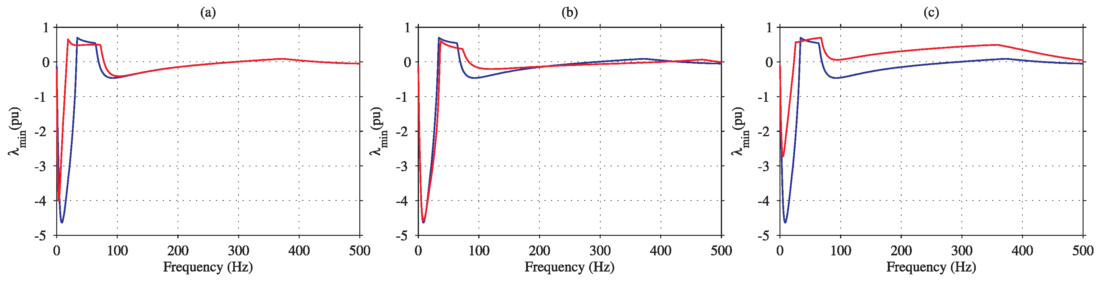
4. Passivity Characterization of the Converter System

In order to evaluate the risk of converter systems in contributing to resonance interactions, passivity theory is used in this paper. If the converter system with its input admittance matrix, ${\mathbf{Y}}_{\mathrm{conv}}$ is passive, i.e., it is stable and $[{\mathbf{Y}}_{\mathrm{conv}}\left(j\omega \right)+{\mathbf{Y}}_{\mathrm{conv}}^{\mathrm{H}}\left(j\omega \right)]\ge 0,\forall \omega$ (i.e., the matrix is positive semidefinite and ${\mathbf{Y}}_{\mathrm{conv}}^{\mathrm{H}}\left(j\omega \right)$ is the Hermitian transpose, which is obtained as the transpose and complex conjugate of the matrix ${\mathbf{Y}}_{\mathrm{conv}}\left(j\omega \right)$), it does not contribute negatively to any resonance interaction in the system. The passivity requirement implies that ${\mathbf{Y}}_{\mathrm{conv}}\left(s\right)$ is stable (which is always the case in this work) and that the minimum eigenvalue, ${\lambda }_{\min }$ of $0.5[{\mathbf{Y}}_{\mathrm{conv}}\left(j\omega \right)+{\mathbf{Y}}_{\mathrm{conv}}^{\mathrm{H}}\left(j\omega \right)]$ is non-negative $\forall \omega$ [13].

To evaluate the impact of control parameters, the control settings as in Table 1 are selected. The control parameters are tuned to obtain a closed-loop bandwidth of 6 Hz for the power controllers and 300 Hz for the current controller. In addition, the virtual impedance is chosen the same as the impedance of the phase reactor as $L_{\mathrm{v}}=L_{\mathrm{f}}$ and $R_{\mathrm{v}}=R_{\mathrm{f}}$, where $L_{\mathrm{f}}=0.15$ pu and $R_{\mathrm{f}}=0.015$ pu. Finally, a sampling time and control delay of $T_{\mathrm{samp}}=0.4$ ms and $T_{\mathrm{cont}}=0.2$ ms, respectively, are considered.

4.1. Impact of Operating Point

The first test is to investigate the impact of operating point on the passivity properties of the converter. Figure 3 shows the passivity index, ${\lambda }_{\min }$ for a variation of both active and reactive power. As the results indicate, the impact of operating points is not significant and is only visible for a small frequency interval in the low-frequency range for the case of active power. For this reason, the impact of operating point can be assumed negligible (i.e., $i_{\mathrm{f}0}^d=i_{\mathrm{f}0}^q=0\Rightarrow {\mathbf{G}}_{\mathrm{D}}=H_{\mathrm{d}}[01;E_{\mathrm{g}}0]$, and ${\mathbf{G}}_{\mathrm{PQv}}=\mathbf{0}$) for the majority of the frequency intervals and a simplified expression for (8) can be obtained as

$${\mathbf{Y}}_{\mathrm{conv}}={[H_{\mathrm{d}}{\mathbf{G}}_{\mathrm{cc}}^{\mathrm{mat}}-H_{\mathrm{d}}G{}_{\mathrm{cc}}{\mathbf{Z}}_{\mathrm{v}}^{-1}{\mathbf{G}}_{\mathrm{PQ}}^{{}^{\prime }}+{\mathbf{Z}}_{\mathrm{f}}]}^{-1}\left[H_{\mathrm{d}}G{}_{\mathrm{cc}}{\mathbf{Z}}_{\mathrm{v}}^{-1}+\left(1-H_{\mathrm{d}}{H}_{\mathrm{ff}}\right)\mathbf{I}\right]$$

(10)

where ${\mathbf{G}}_{\mathrm{PQ}}^{{}^{\prime }}$ is given by

$${\mathbf{G}}_{\mathrm{PQ}}^{{}^{\prime }}=\left[\begin{array}{c}\begin{array}{cc}0& H_{\mathrm{fm}}{G}_{\mathrm{Qc}}{E}_{\mathrm{g}}\end{array}\\ \begin{array}{cc}& \end{array}\\ \begin{array}{cc}-H_{\mathrm{fm}}{G}_{\mathrm{Pc}}{E}_{\mathrm{g}}^2& 0\end{array}\end{array}\right]$$

(11)

Figure 3. (a) Frequency response of the index ${\lambda }_{\min }$ for $Q_{\mathrm{g}0}=0$, and $P_{\mathrm{g}0}=1$ pu (blue), $P_{\mathrm{g}0}=0$ pu (green), $P_{\mathrm{g}0}=-1$ pu (red); (b) frequency response of the index ${\lambda }_{\min }$ for $P_{\mathrm{g}0}=0$, and $Q_{\mathrm{g}0}=0.5$ pu (blue), $Q_{\mathrm{g}0}=0$ pu (green), $Q_{\mathrm{g}0}=-0.5$ pu (red).

It is important to observe that all the matrices in (10) are symmetric except for ${\mathbf{G}}_{\mathrm{PQ}}^{{}^{\prime }}$. This means that with a proper choice for the active- and reactive-power controllers, ${\mathbf{G}}_{\mathrm{Pc}}$ and ${\mathbf{G}}_{\mathrm{Qc}}$, it is possible to symmetrize the matrix, ${\mathbf{G}}_{\mathrm{PQ}}^{{}^{\prime }}$ and hence a SISO representation for (10) is possible as it will be shown later.

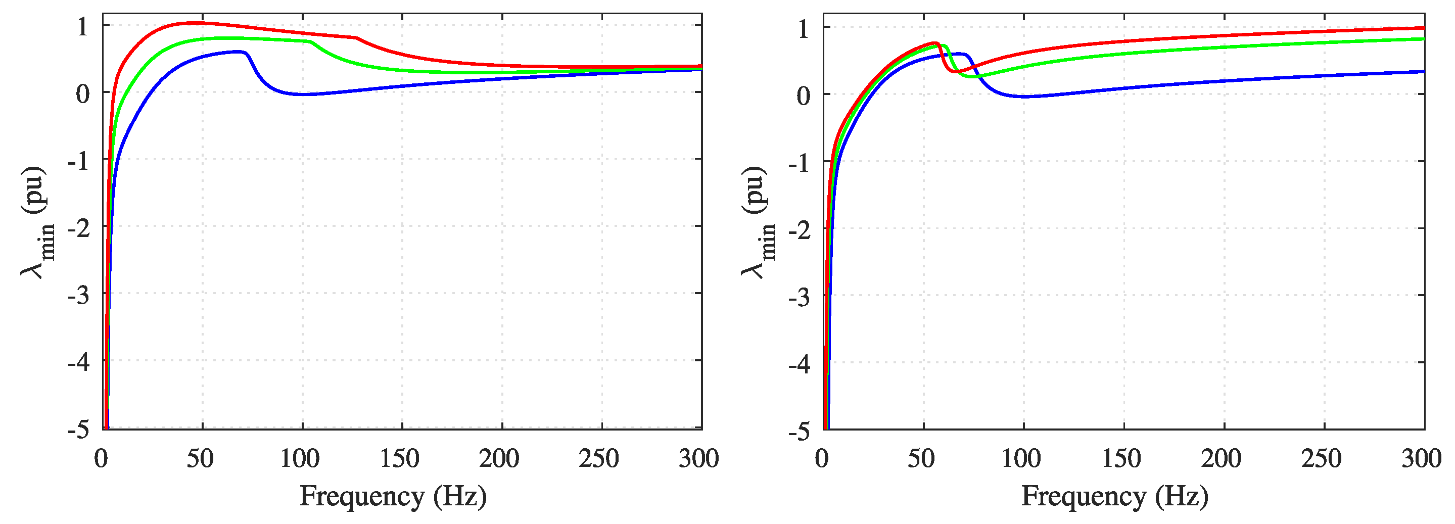
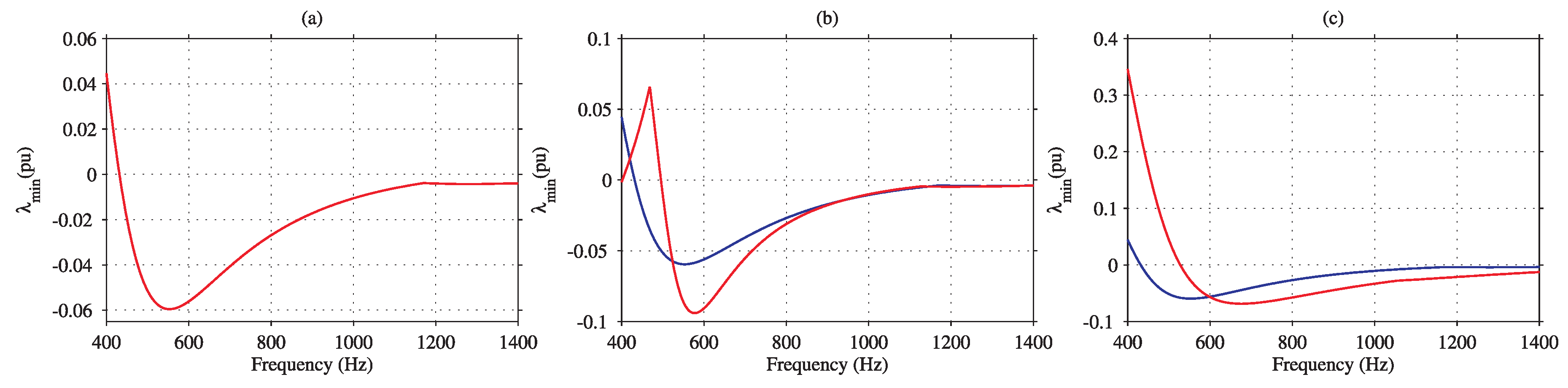
4.2. Impact of Control Parameters

It can be observed from Figure 3 that non-passive behavior for the converter system exists at low-, medium- and high-frequency intervals and the various factors attributing to this are explained in this section. Medium-frequency refers to intervals close to and around the current controller bandwidth. Low- and high-frequency refers to intervals lower and higher than the medium-frequency interval, respectively. For this purpose, the impact of the control bandwidth for the power and current controllers as well as parameters of the virtual impedance on the passivity properties of the converter are demonstrated in Figure 4 and Figure 5. Note that these figures are plotted for two frequency intervals to highlight the impact of the control parameters in the low- and high-frequency ranges.

Figure 4. Frequency characteristics of the index ${\lambda }_{\min }$ from 0–500 Hz with variation in control parameters; (a) closed-loop bandwidth for the power controllers as 6 Hz (blue) and 3 Hz (red); (b) closed-loop bandwidth for the current controller as 300 Hz (blue) and 450 Hz (red); and (c) parameters of the virtual impedance as $R_{\mathrm{v}}=R_{\mathrm{f}}$, $L_{\mathrm{v}}=L_{\mathrm{f}}$ (blue) and $R_{\mathrm{v}}=1.5R_{\mathrm{f}}$, $L_{\mathrm{v}}=1.5L_{\mathrm{f}}$ (red).

Figure 5. Frequency characteristics of the index ${\lambda }_{\min }$ from 400–1400 Hz with variation in control parameters; (a) closed-loop bandwidth for the power controllers as 6 Hz (blue) and 3 Hz (red); (b) closed-loop bandwidth for the current controller as 300 Hz (blue) and 450 Hz (red); and (c) parameters of the virtual impedance as $R_{\mathrm{v}}=R_{\mathrm{f}}$, $L_{\mathrm{v}}=L_{\mathrm{f}}$ (blue) and $R_{\mathrm{v}}=1.5R_{\mathrm{f}}$, $L_{\mathrm{v}}=1.5L_{\mathrm{f}}$ (red).

From the results, it can be understood that the power controllers have an impact in the low-frequency range only, where a higher bandwidth results in a more non-passive behavior. This implies that passivity improvement comes at a cost of reduced speed of response. The impact of the current controller bandwidth in the low- and medium-frequency interval is inconclusive and is not an effective way to improve passivity in that frequency range. On the other hand, an increase in the current controller bandwidth results in a more non-passive behavior at high frequency, which again implies that passivity improvement comes at a cost of reduced speed of response. Finally, it can be observed from the results that the parameters of the virtual impedance have a significant impact on the passivity property at all frequency intervals, where higher values improve the passivity in the low- and medium-frequency range and reduce the passivity at high-frequency range. This indicates that a proper tuning of the parameters of the virtual impedance can provide the flexibility to improve passivity without deteriorating the speed of response for the power or the current controllers. This will be addressed in a later section, following after a demonstration of the impact of the passivity property of the converter system on resonance instability through simulation and experimental tests.

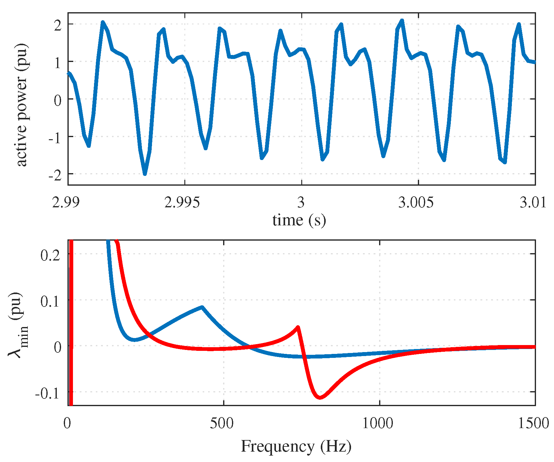
4.3. Simulation Study

The impact of passivity on the stability of a converter-grid system as in Figure 1 using time-domain simulations is demonstrated here. For this, the impact of varying the parameters of the virtual impedance is considered with a connecting grid as shown in Figure 6, which represents the network to the right of the measured grid-voltage, $e_{\mathrm{g}}$ in Figure 1. The parameters are chosen as $L_{\mathrm{g}}=0.25$, $R_{\mathrm{g}}=0.025$, $C_{\mathrm{g}1}=0.25$, $L_{\mathrm{g}1}=0.025$, $R_{\mathrm{g}1}=0.0025$, $L_{\mathrm{t}}=0.1$ and $C_{\mathrm{f}}=0.15$ pu to obtain a grid resonance as shown in Figure 7 (plot a). As the result in Figure 7 (plot b) shows, the converter-grid system is stable with a converter control employing higher virtual impedance value resulting in a more passive converter system around the grid-resonance frequency as shown in Figure 4 (plot c). For lower values of the virtual-admittance parameters, the input admittance presents a non-passive region around the grid resonance, which results in the instability as shown in the growing oscillations in the output power.

Figure 6. Schematics of the connecting grid showing the input-impedance, $Z_{\mathrm{grid}}$ together with its comprising passive components for investigating resonance instability.

Figure 7. Impact of virtual impedance on converter-grid stability; (a) magnitude of grid impedance (b) active-power output of the converter when $R_{\mathrm{v}}=R_{\mathrm{f}}$, $L_{\mathrm{v}}=L_{\mathrm{f}}$ for the time interval 1 s to 1.05 s and $R_{\mathrm{v}}=1.5R_{\mathrm{f}}$, $L_{\mathrm{v}}=1.5L_{\mathrm{f}}$ for other times.

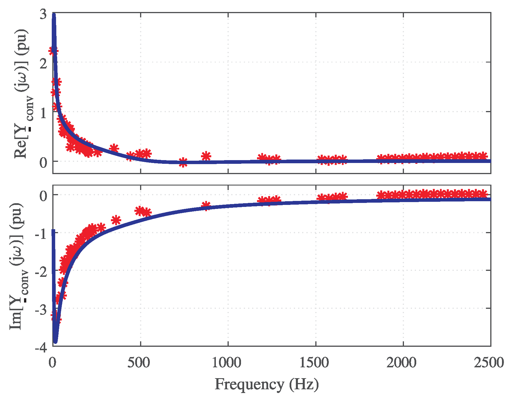
5. Experimental Validation

The findings in the previous section on the analytical model of the converter system input admittance as well as a demonstration of resonance instability are validated in a small-scale laboratory setup similar to the one in Figure 1. For this, a 30 kVA Regatron 4-quadrant controllable power supply is used to emulate the Thévenin equivalent of the connecting grid. A two-level converter system rated 1 kVA, 100 V is then connected to the emulated grid through a phase reactor with $L_{\mathrm{f}}=0.16$ pu and $R_{\mathrm{f}}=0.05$ pu to make the various tests. A dc source with voltage 300 V is connected on the dc-side of the converter and a switching frequency of 5 kHz is used. The converter is controlled by a dSPACE DS1103 processor board, where a sampling frequency of 5 kHz is applied.

5.1. Input-Admittance Verification

An approximated single-input single-output system (SISO) representation of the input-admittance matrix relating the $dq$-current and voltage components is used here for the purpose of verifying the analytical models with experimental models in this section. This SISO-approximated admittance model (${\underline{Y}}_{\mathrm{conv}}$) is obtained from the input admittance matrix, ${\mathbf{Y}}_{\mathrm{conv}}$ in (8) as [13]

$${\underline{Y}}_{\mathrm{conv}}=0.5\left(\left[{\mathbf{Y}}_{\mathrm{conv}}(1,1)+{\mathbf{Y}}_{\mathrm{conv}}(2,2)\right]+j\left[{\mathbf{Y}}_{\mathrm{conv}}(2,1)-{\mathbf{Y}}_{\mathrm{conv}}(1,2)\right]\right)$$

(12)

To obtain the input admittance from the experimental setup, a voltage perturbation is made from the Regatron Grid Simulator at various frequencies. For each perturbation, the resulting perturbation $dq$-component currents from the converter system are measured, and the input admittance matrix is extracted using DFT calculations. From the admittance matrix, the SISO-approximated admittance model as in (12) is extracted for comparison with the corresponding analytical model. As the results in Figure 8 indicate, the analytical and experimental models show a good match confirming the validity of the analytical model in (8). It is important to note that this SISO-approximated admittance model is used only for the purpose of this verification for simplicity and is not applied in the analysis that came before this section or the ones that follow.

Figure 8. Input admittance for the analytical model (blue) and experiment (red); parameters: $T_{\mathrm{samp}}$ = $T_{\mathrm{cont}}$ = 0.2 ms, bandwidth of the power controllers 3 Hz, power-measurement filter 30 Hz, current controller 300 Hz, voltage feedforward filter 30 Hz, and $R_{\mathrm{v}}=R_{\mathrm{f}}$, $L_{\mathrm{v}}=L_{\mathrm{f}}$.

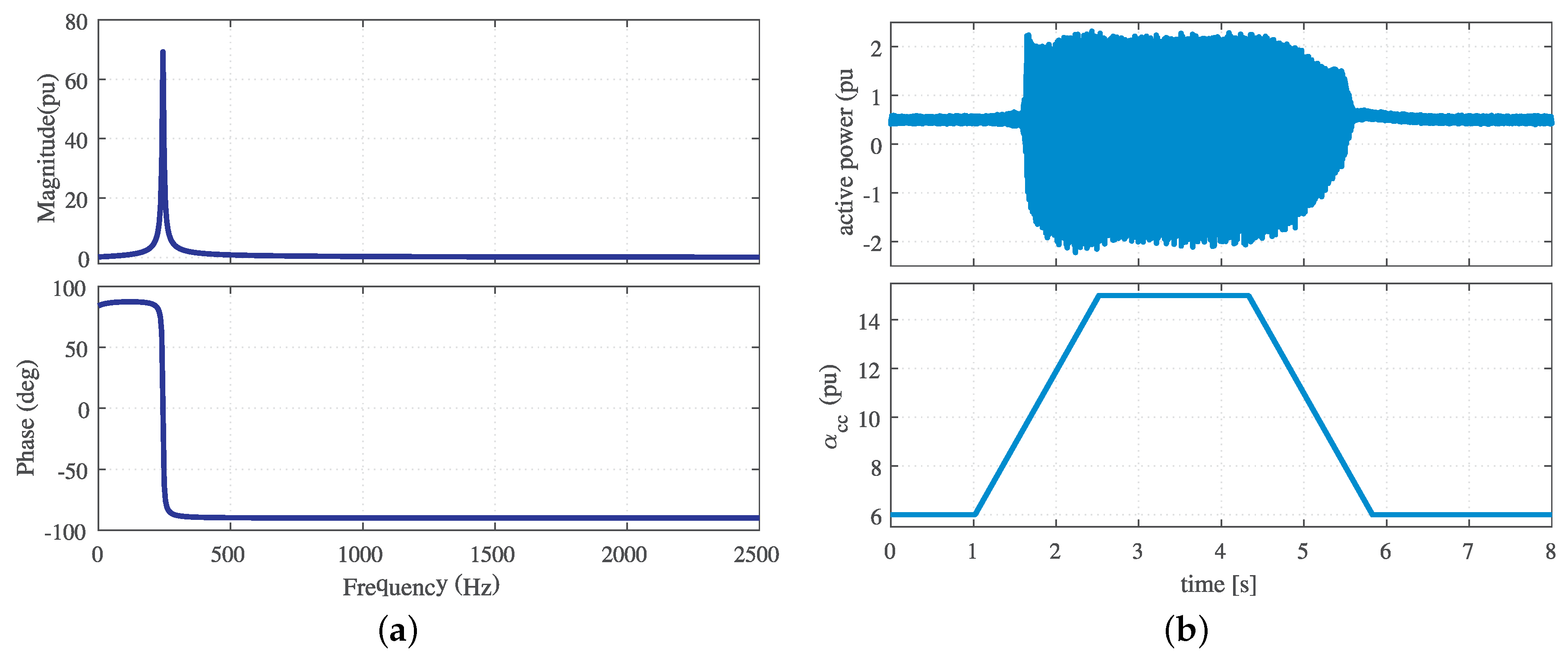
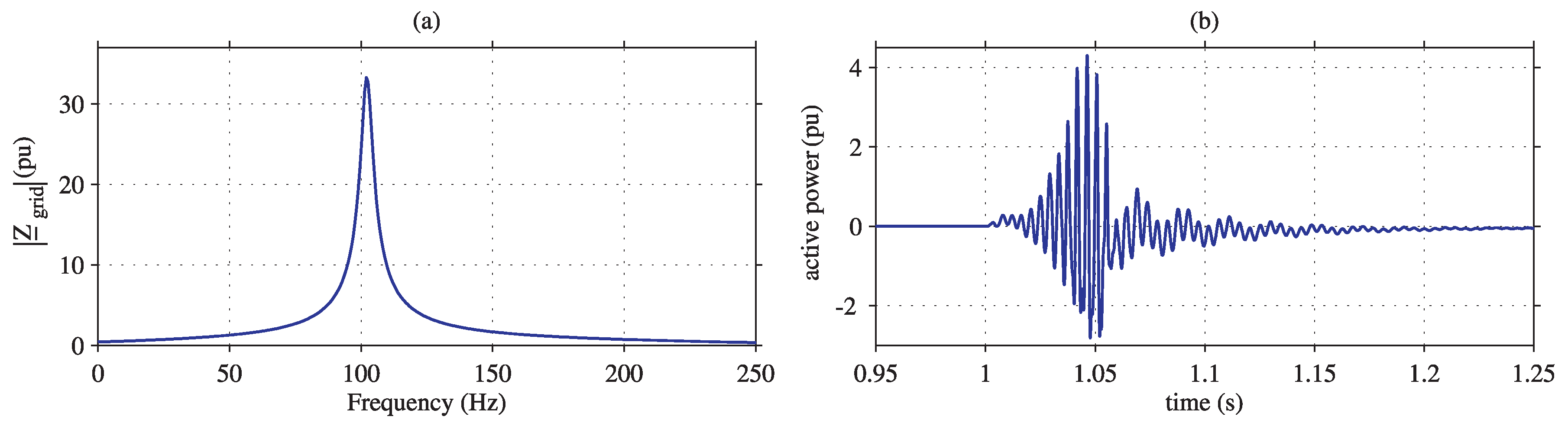
5.2. Resonance Instability Study

The impact of control parameters on the passivity of a converter system and as a result on the stability of an interconnected converter-grid system will be verified experimentally in this section. For this purpose, a simplified connecting grid consisting of only passive components as in Figure 6 is considered so that any resonance-interaction phenomena can be attributed to the non-passive characteristics of the converter system. With a demonstration of low-frequency resonance instability included in the simulation section, the phenomenon of resonance instability at a higher frequency is shown here. Hence, the parameters for the connecting grid are tuned to obtain instead a grid resonance close to 250 Hz as shown in Figure 9a.

Figure 9. (a) Frequency response of the connection-grid impedance, ${\underline{Z}}_{\mathrm{grid}}$; (b) active-power output of the converter with a resonance grid connection and $R_{\mathrm{v}}=R_{\mathrm{f}}$, $L_{\mathrm{v}}=L_{\mathrm{f}}$ during a change in the current-controller bandwidth, ${\alpha }_{\mathrm{cc}}$.

The risk for instability can be predicted from observation of the passivity index, ${\lambda }_{\min }$ as described in the previous section, see Figure 4 and Figure 5. It has been shown that the presence of a current controller presents a significant non-passive region at high frequency, presenting a higher risk for resonance instability. To verify this, the impact of increasing the current controller bandwidth in the grid-forming control strategy is investigated and the results are shown in Figure 9b.

As can be observed from the active power plot, a change in the current controller bandwidth results in resonance instability. This is attributed to the non-passive behavior presented by the converter system as well as the closeness of this non-passive behavior to the grid resonance. To investigate this, the oscillation in the active-power output is plotted in detail in Figure 10 (top plot) and it can be estimated that the unstable oscillation is close to 400 Hz. For this resonance instability to happen, a non-passive property must exist around this oscillation frequency as the current-controller bandwidth changes. Hence, the passivity index is plotted for two values of the current-controller bandwidth in Figure 10 (bottom plot).

Figure 10. Top: oscillation in active-power output of the converter with a resonance grid connection during a change in the current-controller bandwidth; bottom: frequency response of the passivity index ${\lambda }_{\min }$; the bandwidth of the current controller is chosen at 6 pu (blue curve) and 15 pu (red curve).

As can be seen clearly, the increase in the bandwidth of the current controller results in a non-passive region for frequency intervals 330–620 Hz and above 750 Hz. With a non-passive property in the converter system in a given frequency interval, the overall stability of the connected system is dependent on the availability of enough positive damping from the grid subsystem. To demonstrate the risk of instability that comes with the existence of a non-passive property of the converter system, a grid with resonance around 250 Hz is considered as shown in Figure 9a. This means that the grid system will have the smallest damping contribution to the interconnected system at the resonance pick even though the converter system is passive at this particular frequency. As the resonance peak is not sharp and, as a result, the minimal damping contribution from the grid is extended well above 250 Hz into the active region of the converter system in the interval 330–620 Hz. This causes the instability to fall in the region of 400 Hz as indicated in Figure 10.

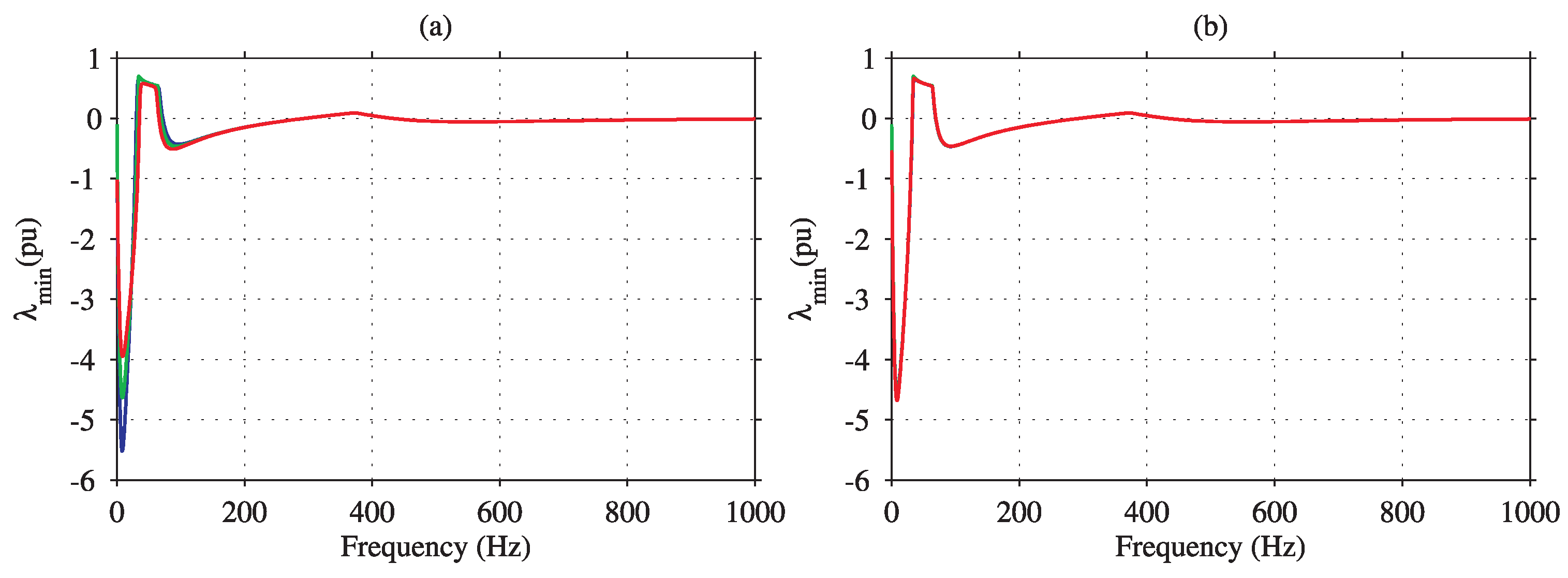
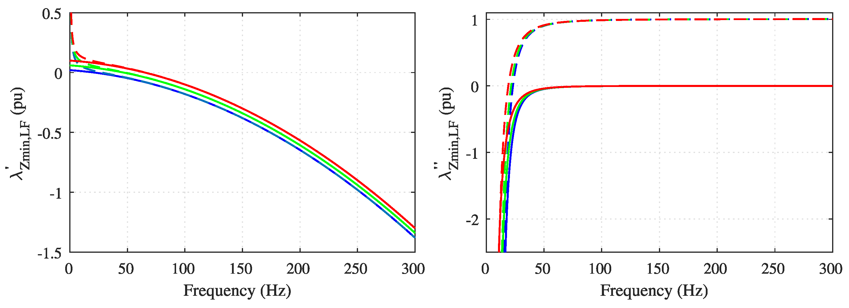
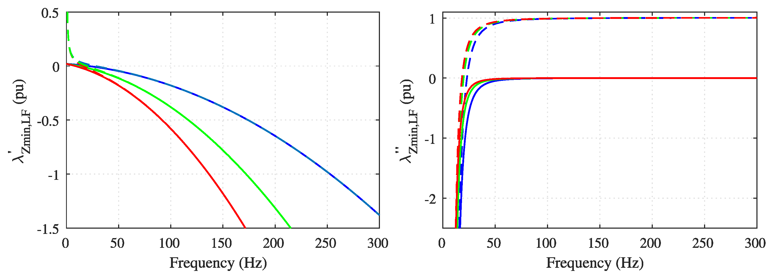
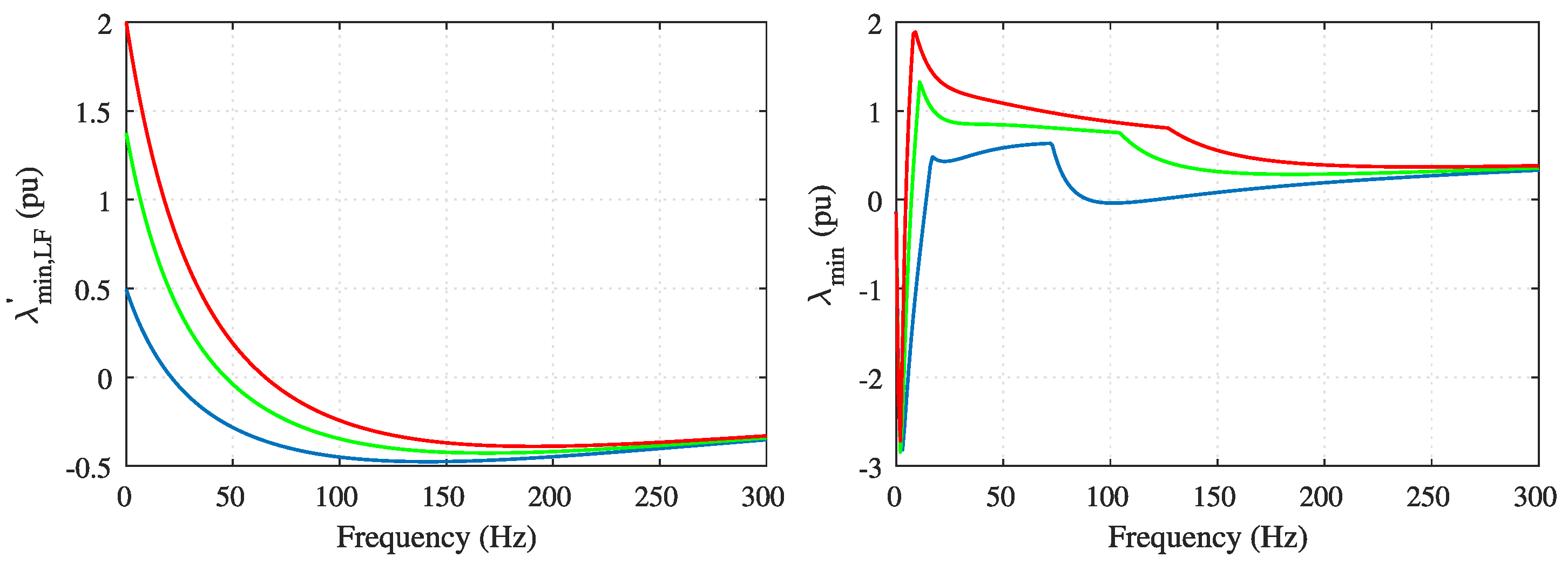
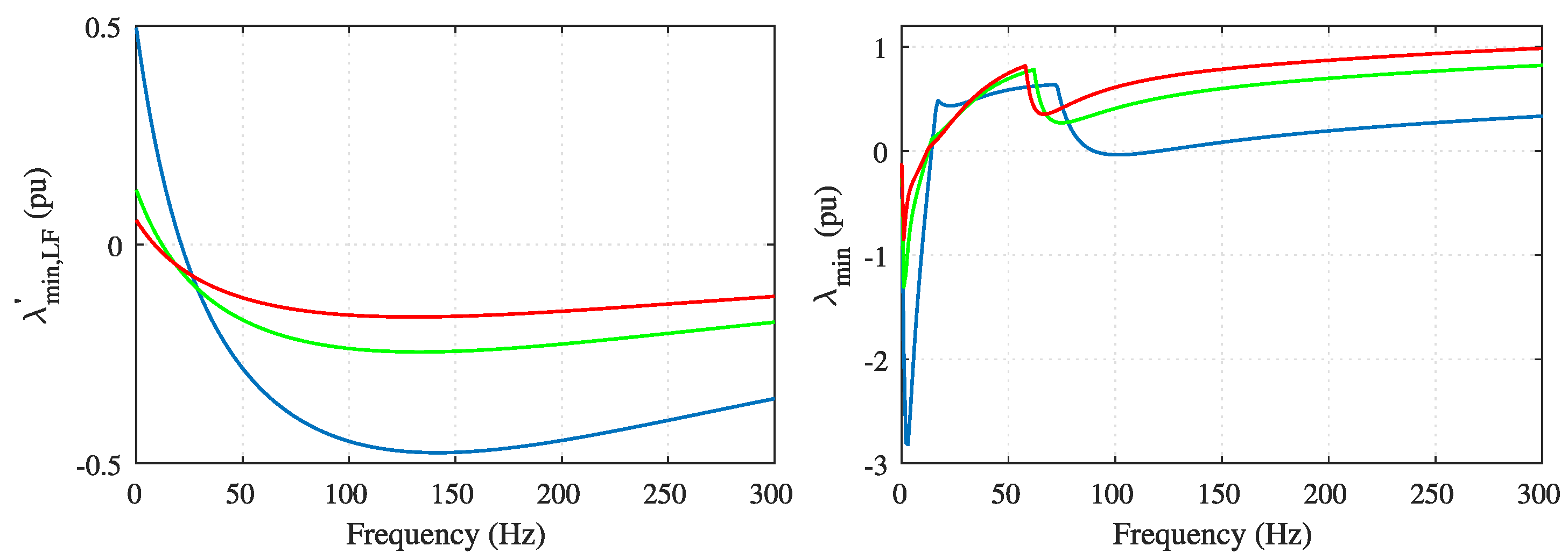
6. Passivity Improvement through Tuning of Virtual-Impedance Parameters

It has been shown that the presence of a non-passive region in the converter system impacts the overall stability of the system analytically and through simulation and experimental tests in previous sections. As a result, increasing the passivity of one of the subsystems is paramount in ensuring the stability of the interconnected system. Hence, this section focuses on achieving this purpose through tuning of virtual-impedance parameters. It has been shown that non-passive properties of the converter system are mainly attributed to the current controller with the converter delays in the high-frequency range and to the power controllers in the low-frequency range. On the other hand, the impact of the virtual impedance is visible both in the low- and high-frequency intervals. In this section, the choice of the virtual impedance parameters to improve passivity is discussed, where simplification of the input admittance is made as required. For this purpose, without loss of generality, the active- and reactive-power controllers are chosen such that the matrix, $G_{\mathrm{PQ}}^{{}^{\prime }}$ in (11) is symmetric, i.e., $G_{\mathrm{Qc}}=G_{\mathrm{Pc}}{E}_{\mathrm{g}}\Rightarrow {\alpha }_{\mathrm{Pc}}={\alpha }_{\mathrm{Qc}}$ based on the basic structure in Table 1. This results in the input-admittance matrix in (10) to be symmetric and an equivalent complex SISO input admittance, ${\underline{Y}}_{\mathrm{conv}}$ to be derived as

$$\begin{array}{ccc}{\underline{Y}}_{\mathrm{conv}}\hfill & =& [H_{\mathrm{d}}(G_{\mathrm{cc}}-j\omega {}_1{L}_{\mathrm{f}})+s{L}_{\mathrm{f}}+R_{\mathrm{f}}+j\omega {}_1{L}_{\mathrm{f}}+\dots \\ \hfill & & j{H}_{\mathrm{d}}G{}_{\mathrm{cc}}{H}_{\mathrm{fm}}{G}_{\mathrm{Qc}}{E}_{\mathrm{g}}/{\underline{Z}}_{\mathrm{v}}{]}^{-1}\left[H_{\mathrm{d}}G{}_{\mathrm{cc}}/{\underline{Z}}_{\mathrm{v}}+1-H_{\mathrm{d}}{H}_{\mathrm{ff}}\right]\end{array}$$

(13)

where ${\underline{Z}}_{\mathrm{v}}$ is the complex virtual impedance and for a restive-inductive impedance is given by ${\underline{Z}}_{\mathrm{v}}=R_{\mathrm{v}}+s{L}_{\mathrm{v}}+j{\omega }_1{L}_{\mathrm{v}}$. Hence, the passivity index (${\lambda }_{\min }$) can be obtained from the real value of the input admittance as ${\lambda }_{\min }=\mathrm{Re}\left({\underline{Y}}_{\mathrm{conv}}\left(j\omega \right)\right)$.

6.1. Low-Frequency Passivity Enhancement

Neglecting the impact of the converter delays in the low-frequency range (i.e., $H_{\mathrm{d}}=1$), further simplification of the input-admittance model in (13) can be obtained as

$$\begin{array}{lll}{\underline{Y}}_{\mathrm{conv},\mathrm{LF}}\hfill & =& {[{\underline{Z}}_{\mathrm{v}}\left(1+\left(s{L}_{\mathrm{f}}+R_{\mathrm{f}}\right)/\phantom{\left(s{L}_{\mathrm{f}}+R_{\mathrm{f}}\right)G_{\mathrm{cc}}}{G}_{\mathrm{cc}}\right)+j{H}_{\mathrm{fm}}{G}_{\mathrm{Qc}}{E}_{\mathrm{g}}]}^{-1}\left[1+{\underline{Z}}_{\mathrm{v}}\left(1-H_{\mathrm{ff}}\right)/\phantom{\left(1-H_{\mathrm{ff}}\right)G_{\mathrm{cc}}}{G}_{\mathrm{cc}}\right]\\ \hfill & =& {\left[{\underline{Z}}_{\mathrm{conv},\mathrm{LF}}^{{}^{\prime }}\right]}^{-1}+{\left[{\underline{Z}}_{\mathrm{conv},\mathrm{LF}}^{{}^{″}}\right]}^{-1}\end{array}$$

(14)

where the input admittance is expressed as a parallel connection of two input impedances, ${\underline{Z}}_{\mathrm{conv},\mathrm{LF}}^{{}^{\prime }}$ and ${\underline{Z}}_{\mathrm{conv},\mathrm{LF}}^{{}^{″}}$, given by

$$\begin{array}{l}{\underline{Z}}_{\mathrm{conv},\mathrm{LF}}^{{}^{\prime }}={\underline{Z}}_{\mathrm{v}}\left(1+\left(s{L}_{\mathrm{f}}+R_{\mathrm{f}}\right)/\phantom{\left(s{L}_{\mathrm{f}}+R_{\mathrm{f}}\right)G_{\mathrm{cc}}}{G}_{\mathrm{cc}}\right)+j{H}_{\mathrm{fm}}{G}_{\mathrm{Qc}}{E}_{\mathrm{g}}\hfill \\ {\underline{Z}}_{\mathrm{conv},\mathrm{LF}}^{{}^{″}}=\left(G_{\mathrm{cc}}+s{L}_{\mathrm{f}}+R_{\mathrm{f}}\right)/\phantom{\left(G_{\mathrm{cc}}+s{L}_{\mathrm{f}}+R_{\mathrm{f}}\right)\left(1-H_{\mathrm{ff}}\right)}\left(1-H_{\mathrm{ff}}\right)+j{G}_{\mathrm{cc}}{H}_{\mathrm{fm}}{G}_{\mathrm{Qc}}{E}_{\mathrm{g}}/\phantom{j{G}_{\mathrm{cc}}{H}_{\mathrm{fm}}{G}_{\mathrm{Qc}}{E}_{\mathrm{g}}\left[{\underline{Z}}_{\mathrm{v}}\left(1-H_{\mathrm{ff}}\right)\right]}\left[{\underline{Z}}_{\mathrm{v}}\left(1-H_{\mathrm{ff}}\right)\right]\hfill \end{array}$$

(15)

Hence, passivity enhancement can be achieved by increasing the real part of the two input impedances. Using the control setting in Table 1, the passivity indexes for the two input impedances, ${\lambda }_{\mathrm{Zmin},\mathrm{LF}}^{{}^{\prime }}$ and ${\lambda }_{\mathrm{Zmin},\mathrm{LF}}^{{}^{″}}$ are expressed as

$${\lambda }_{\mathrm{Zmin},\mathrm{LF}}^{{}^{\prime }}=\mathrm{Re}{\left({\underline{Z}}_{\mathrm{conv},\mathrm{LF}}^{{}^{\prime }}\right)}_{s=j\omega }=\underset{\exp -1}{\underbrace{\left[R_{\mathrm{v}}-\frac{L_{\mathrm{v}}}{{\alpha }_{\mathrm{cc}}}\omega (\omega +{\omega }_1)\right]}}+\underset{\exp -2}{\underbrace{\left[\frac{{\alpha }_{{}_{\mathrm{fm}}}^2{\alpha }_{\mathrm{Qc}}{\omega }_1{L}_{\mathrm{f}}}{\omega \left({\omega }^2+{\alpha }_{{}_{\mathrm{fm}}}^2\right)}\right]}}$$

(16)

$$\begin{array}{lll}{\lambda }_{\min ,\mathrm{LF}}^{{}^{″}}\hfill & =& \mathrm{Re}{\left({\underline{Z}}_{\mathrm{conv},\mathrm{LF}}^{{}^{″}}\right)}_{\genfrac{}{}{0pt}{}{s=j\omega \hfill }{{\alpha }_{\mathrm{ff}}\approx {\alpha }_{\mathrm{fm}}\hfill }}\\ \hfill & =& \underset{\exp -1}{\underbrace{\left[{\displaystyle \frac{-{\alpha }_{\mathrm{cc}}{\alpha }_{\mathrm{fm}}{\alpha }_{\mathrm{Qc}}{\omega }_1{L}_{\mathrm{f}}^2}{R_{\mathrm{v}}{\omega }^3}}{\displaystyle \frac{\left(R_{\mathrm{f}}/\phantom{R_{\mathrm{f}}{L}_{\mathrm{f}}+\omega (\omega +{\omega }_1)\left(L_{\mathrm{v}}/\phantom{L_{\mathrm{v}}{R}_{\mathrm{v}}}{R}_{\mathrm{v}}\right)}{L}_{\mathrm{f}}+\omega (\omega +{\omega }_1)\left(L_{\mathrm{v}}/\phantom{L_{\mathrm{v}}{R}_{\mathrm{v}}}{R}_{\mathrm{v}}\right)\right)}{1+{(\omega +{\omega }_1)}^2{\left(L_{\mathrm{v}}/\phantom{L_{\mathrm{v}}{R}_{\mathrm{v}}}{R}_{\mathrm{v}}\right)}^2}}\right]}}+\dots \\ \hfill & & \underset{\exp -2}{\underbrace{\left[R_{\mathrm{f}}+L_{\mathrm{f}}\left({\alpha }_{\mathrm{cc}}+{\alpha }_{\mathrm{fm}}\right)-{\displaystyle \frac{{\alpha }_{\mathrm{cc}}{\alpha }_{\mathrm{fm}}{R}_{\mathrm{f}}}{{\omega }^2}}\right]}}\end{array}$$

(17)

To obtain a methodology for providing a positive contribution from the selection of the virtual-impedance parameters, the frequency characteristic of ${\lambda }_{\mathrm{Zmin},\mathrm{LF}}^{{}^{\prime }}$ and ${\lambda }_{\mathrm{Zmin},\mathrm{LF}}^{{}^{″}}$ are studied in Figure 11 and Figure 12. The frequency characteristics are also plotted considering the first terms only in (16) and (17) where the impact of virtual-impedance parameters exists in the expressions.

Figure 11. Frequency characteristic of ${\lambda }_{\mathrm{Zmin},\mathrm{LF}}^{{}^{\prime }}$ (left) and ${\lambda }_{\mathrm{Zmin},\mathrm{LF}}^{{}^{″}}$ (right) with $L_{\mathrm{v}}=0.2$ pu and $R_{\mathrm{v}}=0.02$ pu (blue), $R_{\mathrm{v}}=0.06$ pu (green), and $R_{\mathrm{v}}=0.10$ pu (red); solid curves represent the case of considering only the virtual-impedance dependent term (exp-1) from ${\underline{Z}}_{\mathrm{conv},\mathrm{LF}}^{{}^{\prime }}$ and ${\underline{Z}}_{\mathrm{conv},\mathrm{LF}}^{{}^{″}}$.

Figure 12. Frequency characteristic of ${\lambda }_{\mathrm{Zmin},\mathrm{LF}}^{{}^{\prime }}$ (left) and ${\lambda }_{\mathrm{Zmin},\mathrm{LF}}^{{}^{″}}$ (right) with $R_{\mathrm{v}}=0.02$ pu and $L_{\mathrm{v}}=0.2$ pu (blue), $L_{\mathrm{v}}=0.4$ pu (green), and $L_{\mathrm{v}}=0.6$ pu (red); solid curves represent the case of considering only the virtual-impedance dependent term (exp-1) from ${\underline{Z}}_{\mathrm{conv},\mathrm{LF}}^{{}^{\prime }}$ and ${\underline{Z}}_{\mathrm{conv},\mathrm{LF}}^{{}^{″}}$.

As the results indicate, the virtual-impedance dependent term, exp-1 in (16), has an impact on the frequency intervals above 25 Hz whereas the second term, exp-2 in (16), has an impact below 25 Hz in the case of ${\lambda }_{\mathrm{Zmin},\mathrm{LF}}^{{}^{\prime }}$. On the other hand, the virtual-impedance dependent term, exp-1 in (17), has an impact on frequency intervals below 25 Hz and the second term, exp-2 in (17), has an impact above 25 Hz in the case of ${\lambda }_{\mathrm{Zmin},\mathrm{LF}}^{{}^{″}}$. This indicates that for a majority of the frequency interval above 25 Hz, the term containing the virtual-impedance parameters in the expression of ${\lambda }_{\mathrm{Zmin},\mathrm{LF}}^{{}^{\prime }}$ in (16) can be an effective term for passivity enhancement. Hence, the corresponding admittance for this purpose containing only the virtual-impedance dependent term, exp-1 in (16) is given by

$$\begin{array}{lll}{\underline{Y}}_{\mathrm{conv},\mathrm{LF}}^{{}^{\prime }}\hfill & =& {\left[{\underline{Z}}_{\mathrm{v}}\left(1+\left(s{L}_{\mathrm{f}}+R_{\mathrm{f}}\right)/\phantom{\left(s{L}_{\mathrm{f}}+R_{\mathrm{f}}\right)G_{\mathrm{cc}}}{G}_{\mathrm{cc}}\right)+j{H}_{\mathrm{fm}}{G}_{\mathrm{Qc}}{E}_{\mathrm{g}}\right]}^{-1}\\ \hfill & \approx & {\left[{\underline{Z}}_{\mathrm{v}}\left(1+\left(s{L}_{\mathrm{f}}+R_{\mathrm{f}}\right)/\phantom{\left(s{L}_{\mathrm{f}}+R_{\mathrm{f}}\right)G_{\mathrm{cc}}}{G}_{\mathrm{cc}}\right)\right]}^{-1}\end{array}$$

(18)

where the corresponding passivity index, ${\lambda }_{\min ,\mathrm{LF}}^{{}^{\prime }}$ is given by

$${\lambda }_{\min ,\mathrm{LF}}^{{}^{\prime }}=\mathrm{Re}{\left({\underline{Y}}_{\mathrm{conv},\mathrm{LF}}^{{}^{\prime }}\right)}_{s=j\omega }\approx \frac{R_{\mathrm{v}}-L_{\mathrm{v}}\left(\omega +{\omega }_1\right)\omega /\phantom{\omega {\alpha }_{\mathrm{cc}}}{\alpha }_{\mathrm{cc}}}{{\left(R_{\mathrm{v}}-L_{\mathrm{v}}\left(\omega +{\omega }_1\right)\omega /\phantom{\omega {\alpha }_{\mathrm{cc}}}{\alpha }_{\mathrm{cc}}\right)}^2+{\left(L_{\mathrm{v}}\left(\omega +{\omega }_1\right)\right)}^2}$$

(19)

Passivity enhancement can be achieved by making the passivity index, ${\lambda }_{\min ,\mathrm{LF}}^{{}^{\prime }}$ as high as possible with the choice of the virtual-impedance parameters. This is obtained through an increase in the value of the virtual resistance and inductance as indicated in Figure 13 and Figure 14. It can be observed that an increase in $R_{\mathrm{v}}$ increases the passivity index and decrease the non-passive frequency interval. The impact of $L_{\mathrm{v}}$ on the other hand is to increase the magnitude of the passivity index without affecting the non-passive region significantly. Thus, the virtual resistance is the most significant parameter to enhance passivity in the low-frequency range. Note that the virtual-impedance parameters should fulfill that the bandwidth of the reference-current estimation in (4) is significantly lower than the current-controller bandwidth. i.e.,

$$R_{\mathrm{v}}/\phantom{R_{\mathrm{v}}{L}_{\mathrm{v}}}{L}_{\mathrm{v}}\ll {\alpha }_{\mathrm{cc}}$$

(20)

Figure 13. Frequency characteristic of ${\lambda }_{\min ,\mathrm{LF}}^{{}^{\prime }}$ (left) and ${\lambda }_{\min }$ (right) with $L_{\mathrm{v}}=0.2$ pu and $R_{\mathrm{v}}=0.02$ pu (blue), $R_{\mathrm{v}}=0.06$ pu (green), and $R_{\mathrm{v}}=0.10$ pu (red).

Figure 14. Frequency characteristic of ${\lambda }_{\min ,\mathrm{LF}}^{{}^{\prime }}$ (left) and ${\lambda }_{\min }$ (right) with $R_{\mathrm{v}}=0.02$ pu and $L_{\mathrm{v}}=0.2$ pu (blue), $L_{\mathrm{v}}=0.4$ pu (green), and $L_{\mathrm{v}}=0.6$ pu (red).

It is shown that the findings above are in agreement with the analysis made in the previous section in Figure 4c, where the passivity has improved when increasing $R_{\mathrm{v}}$ and $L_{\mathrm{v}}$ by $50\%$. The improvement in passivity with this choice is also verified through the simulation demonstration in Figure 7b. The results so far and the conclusion on passivity enhancement through selection of the virtual-impedance parameters have been shown for an active- and reactive-power controller. To show that the results still hold for an active-power and an ac-voltage controller, the impact of virtual-impedance parameters on passivity is shown in Figure 15. As indicated, a similar trend in the passivity is observed.

Figure 15. Left: Frequency characteristic of ${\lambda }_{\min }$ with active-power and ac-voltage controller for $L_{\mathrm{v}}=0.2$ pu and $R_{\mathrm{v}}=0.02$ pu (blue), $R_{\mathrm{v}}=0.06$ pu (green), and $R_{\mathrm{v}}=0.10$ pu (red); Right: Frequency characteristic of ${\lambda }_{\min }$ with active-power and ac-voltage controller for $R_{\mathrm{v}}=0.02$ pu and $L_{\mathrm{v}}=0.2$ pu (blue), $L_{\mathrm{v}}=0.4$ pu (green), and $L_{\mathrm{v}}=0.6$ pu (red).

6.2. Medium- and High-Frequency Passivity Enhancement

For the case of the medium- and high-frequency intervals, neglecting the impact of the power or voltage controllers (i.e., $G_{\mathrm{Pc}}=G_{\mathrm{Qc}}=0$), the input admittance matrix in (13) can be simplified to

$${\underline{Y}}_{\mathrm{conv},\mathrm{HF}}=\frac{\left[H_{\mathrm{d}}{G}_{\mathrm{cc}}+{\underline{Z}}_{\mathrm{v}}\left(1-H_{\mathrm{d}}{H}_{\mathrm{ff}}\right)\right]}{{\underline{Z}}_{\mathrm{v}}\left(H_{\mathrm{d}}{G}_{\mathrm{cc}}+s{L}_{\mathrm{f}}+R_{\mathrm{f}}+j\omega {}_1{L}_{\mathrm{f}}(1-H_{\mathrm{d}})\right)}={\left[{\underline{Z}}_{\mathrm{conv},\mathrm{HF}}^{{}^{\prime }}\right]}^{-1}+{\left[{\underline{Z}}_{\mathrm{conv},\mathrm{HF}}^{{}^{″}}\right]}^{-1}$$

(21)

where the input admittance is expressed as a parallel connection of two input impdances, ${\underline{Z}}_{\mathrm{conv},\mathrm{HF}}^{{}^{\prime }}$ and ${\underline{Z}}_{\mathrm{conv},\mathrm{HF}}^{{}^{″}}$, given by

$$\begin{array}{c}{\underline{Z}}_{\mathrm{conv},\mathrm{HF}}^{{}^{\prime }}={\underline{Z}}_{\mathrm{v}}\left[1+\left(s{L}_{\mathrm{f}}+R_{\mathrm{f}}+j\omega {}_1{L}_{\mathrm{f}}(1-H_{\mathrm{d}})\right)/\phantom{\left(s{L}_{\mathrm{f}}+R_{\mathrm{f}}+j\omega {}_1{L}_{\mathrm{f}}(1-H_{\mathrm{d}})\right)\left(H_{\mathrm{d}}{G}_{\mathrm{cc}}\right)}\left(H_{\mathrm{d}}{G}_{\mathrm{cc}}\right)\right]\hfill \\ {\underline{Z}}_{\mathrm{conv},\mathrm{HF}}^{{}^{″}}=\left(H_{\mathrm{d}}{G}_{\mathrm{cc}}+s{L}_{\mathrm{f}}+R_{\mathrm{f}}+j\omega {}_1{L}_{\mathrm{f}}(1-H_{\mathrm{d}})\right)/\phantom{\left(H_{\mathrm{d}}{G}_{\mathrm{cc}}+s{L}_{\mathrm{f}}+R_{\mathrm{f}}+j\omega {}_1{L}_{\mathrm{f}}(1-H_{\mathrm{d}})\right)\left(1-H_{\mathrm{d}}{H}_{\mathrm{ff}}\right)}\left(1-H_{\mathrm{d}}{H}_{\mathrm{ff}}\right)\hfill \end{array}$$

(22)

Hence, passivity enhancement can be achieved by increasing the real part of the first input impedance, ${\underline{Z}}_{\mathrm{conv},\mathrm{HF}}^{{}^{\prime }}$ which is dependent on ${\underline{Z}}_{\mathrm{v}}$. Using the fact that $R_{\mathrm{f}}\ll \omega L_{\mathrm{f}}$ for medium and high frequency, this passivity index (${\lambda }_{\mathrm{Zmin},\mathrm{HF}}^{{}^{\prime }}$) is expressed as

$$\begin{array}{lll}{\lambda }_{\min ,\mathrm{HF}}^{{}^{\prime }}\hfill & =& \mathrm{Re}\left({\underline{Z}}_{\mathrm{conv},\mathrm{HF}}^{{}^{\prime }}\left(j\omega \right)\right)\\ \hfill & =& {\displaystyle \frac{R_{\mathrm{v}}}{{\alpha }_{\mathrm{cc}}}}\left[{\alpha }_{\mathrm{cc}}-(\omega +{\omega }_1)sin\left(\omega T_{\mathrm{delay}}\right)\right]+\dots \\ \hfill & & {\displaystyle \frac{L_{\mathrm{v}}(\omega +{\omega }_1)}{{\alpha }_{\mathrm{cc}}}}\left[{\omega }_1-(\omega +{\omega }_1)cos\left(\omega T_{\mathrm{delay}}\right)\right]\end{array}$$

(23)

where $T_{\mathrm{delay}}$ represents the total equivalent converter delay. Using (23), the parameters of the virtual impedance can be tuned to maximize the term ${\lambda }_{\min ,\mathrm{HF}}^{{}^{\prime }}$ in the medium- and high-frequency range. However, due to the continuous change of the magnitude and sign of $sin\left(\omega T_{\mathrm{delay}}\right)$ and $cos\left(\omega T_{\mathrm{delay}}\right)$ depending on the frequency, the parameters $R_{\mathrm{v}}$ and $L_{\mathrm{v}}$ should be selected carefully to shape the passivity of the input admittance. In addition, it is important to note that the selection of parameters to enhance passivity at these frequency intervals can have a worsening impact at low-frequency and that should always be considered.

7. Conclusions

The impact of operating point and control loops of a grid-forming control strategy on the passivity behavior of converter systems in the low- and high-frequency range has been investigated in this paper. It has been shown that the impact of steady-state active and reactive power is negligible on the passivity of the input admittance. It has been revealed that a higher bandwidth of the power control loops decreases the passivity property by increasing the non-passive region of the input admittance in the low-frequency range. In the high-frequency range, the current controller and the converter delays have a significant impact on passivity. on the other hand, it has been shown that the virtual impedance has an impact on the passivity of the converter system both at low- and high-frequency intervals. By obtaining simplified input-admittance expressions at various frequency intervals, it has been shown how passivity can be improved through tuning of virtual impedance without compromising control bandwidth. Finally, the findings are verified both through detailed time-domain simulations and experimental tests.

References

1. Zhang, L.; Harnefors, L.; Nee, H.-P. Power-Synchronization Control of Grid-Connected Voltage-Source Converters. IEEE Trans. Power Syst. 2010, 25, 809–820. [Google Scholar] [CrossRef]
2. Zhong, Q.C.; Weiss, G. Synchronverters: Inverters That Mimic Synchronous Generators. IEEE Trans. Ind. Electron. 2011, 54, 1259–1267. [Google Scholar] [CrossRef]
3. Rodriguez, P.; Candela, I.; Citro, C.; Rocabert, J.; Luna, A. Control of grid-connected power converters based on a virtual admittance control loop. In Proceedings of the 2013 15th European Conference on Power Electronics and Applications (EPE), Lille, France, 2–6 September 2013; pp. 1–10. [Google Scholar]
4. Kkuni, K.; Mohan, S.; Yang, G.; Xu, W. Comparative assessment of typical control realizations of grid forming converters based on their voltage source behavior. arXiv 2021, arXiv:2106.10048v1. [Google Scholar]
5. Rodriguez, P.; Candela, I.; Luna, A. Control of PV generation systems using the synchronous power controller. In Proceedings of the 2013 IEEE Energy Conversion Congress and Exposition, Denver, Colorado, 15–19 September 2013; pp. 993–998. [Google Scholar]
6. Watson, J.; Ojo, Y.; Lestas, I.; Spanias, C. Stability of power networks with grid-forming converters. In Proceedings of the 2019 IEEE Milan PowerTech, Milan, Italy, 23–27 June 2019; pp. 1–6. [Google Scholar]
7. Ray, I. Review of Impedance-Based Analysis Methods Applied to Grid-Forming Inverters in Inverter-Dominated Grids. Energies 2021, 14, 2686. [Google Scholar] [CrossRef]
8. Beza, M.; Bongiorno, M. Impact of converter control strategy on low-and high-frequency resonance interactions in power-electronic dominated systems. Int. J. Electr. Power Energy Syst. 2020, 120, 105978. [Google Scholar] [CrossRef]
9. Beza, M.; Bongiorno, M.; Narula, A. Impact of control loops on the low-frequency passivity properties of grid-forming converters. In Proceedings of the 2020 22nd European Conference on Power Electronics and Applications (EPE’20 ECCE Europe), Lyon, France, 7–11 September 2020; pp. 1–10. [Google Scholar]
10. Harnefors, L.; Yepes, A.G.; Vidal, A.; Doval-Gandoy, J. Passivity-Based Controller Design of Grid-Connected VSCs for Prevention of Electrical Resonance Instability. IEEE Trans. Ind. Electron. 2015, 62, 702–710. [Google Scholar] [CrossRef]
11. Liu, H.; Sun, J. Voltage Stability and Control of Offshore Wind Farms with AC Collection and HVDC Transmission. IEEE J. Emerg. Sel. Topics Power Electron. 2014, 2, 1181–1189. [Google Scholar]
12. Amin, M.; Molinas, M. Understanding the Origin of Oscillatory Phenomena Observed Between Wind Farms and HVdc Systems. IEEE J. Emerg. Sel. Topics Power Electron. 2017, 5, 378–392. [Google Scholar] [CrossRef] [Green Version]
13. Beza, M.; Bongiorno, M. Identification of resonance interactions in offshore-wind farms connected to the main grid by MMC-based HVDC system. Int. J. Electr. Power Energy Syst. 2019, 111, 101–113. [Google Scholar] [CrossRef]
14. Li, C.; Liang, J.; Cipcigan, L.; Ming, W.; Colas, F.; Guillaud, X. DQ Impedance Stability Analysis for the Power-Controlled Grid-Connected Inverter. IEEE Trans. Energy Convers. 2020, 2020 35, 1762–1771. [Google Scholar] [CrossRef]
15. Liao, Y.; Wang, X.; Blaabjerg, F. Passivity-Based Analysis and Design of Linear Voltage Controllers For Voltage-Source Converters. IEEE Open J. Ind. Electron. Soc. 2020, 2020 1, 114–126. [Google Scholar] [CrossRef]
16. Liao, Y.; Wang, X. Passivity Analysis and Enhancement of Voltage Control for Voltage-Source Converters. In Proceedings of the 2019 IEEE Energy Conversion Congress and Exposition (ECCE), Baltimore, MD, USA, 29 September–3 October 2019; pp. 5424–5429. [Google Scholar]