Thermal Protection Technology for Acoustic–Magnetic Device in a Geothermal Water Anti-Scaling System

Abstract

This article presents the results of the design of acoustic–magnetic device thermal protection technology based on simulation. The acoustic–magnetic device (AMD) was installed in the heat supply system of a greenhouse complex with a geothermal heat source, developed and patented by the authors of this paper. Simulation was performed to investigate the possibility of maintaining the acoustic transmitter temperature of the acoustic–magnetic device in its operating range. The QuickField Student Edition v 6.4 simulation environment was used for this purpose. Based on the results of the simulation, the optimum thermal mode of the acoustic–magnetic device was developed and implemented. The optimum temporal operating mode of the acoustic–magnetic device is necessary for the optimization of the non-reagent treatment of geothermal water in a heat supply system of a greenhouse complex. It allows for a considerable reduction in the intensity of scale formation in the heat exchanger and equipment of a geothermal heating system. As demonstrated by the simulation thermal modes, the acoustic–magnetic device provides conditions for the work maintenance of the AMD acoustic transmitter at the resonance frequency, reduces the power expenses, and increases the efficiency of the acoustic influence on the scale formed in the heat supply system of a greenhouse complex. The results of the simulation were implemented in the greenhouse complex of JSC “Raduga”. The thermal protection technology was realized by installing two acoustic–magnetic devices and automation systems in the geothermal heating system a greenhouse complex.

1. Introduction

The effective provision of food to populations, considering population growth rates, is an urgent problem of mankind. One of the possible solutions to this problem is the use of greenhouse complexes that allow year-round plant food production [1].

Contemporary greenhouse complexes have microclimate systems. The heat supply subsystem is the basic subsystem necessary for the year-round functioning of a greenhouse complex. There are various ways to heat greenhouses based on solar radiation—the heat generated by heating networks, gas-based boilers, electricity, biofuel boilers, geothermal water, and waste heat of industrial enterprises. The use of geothermal energy is widespread around the world.

A group of authors from Arizona [2] noted that greenhouses play a significant role in modern agriculture, despite the large energy input required for greenhouse heating systems. The solution to this issue, according to the authors, is the use of geothermal power engineering. The authors analyzed the suitability of geothermal heat sources for agricultural needs based on the University of Bari’s experimental farm by measuring the experimental data (greenhouse temperature and heat pump performance). The experimental results from this research confirmed that geothermal heat sources are efficient, economical, and environmentally friendly. Moreover, geothermal heat sources can be useful for meeting the thermal energy demand of greenhouses [3].

The authors of [4] conducted research in remote regions of Canada with a complex environment to provide traditional methods of obtaining a reliable energy supply. The authors proposed geothermal energy as a solution to the prevailing conditions. In addition, they noted the positive aspects of the transition to renewable energy sources in the current ecological situation.

The authors of [5] noted that the geographic location of Turkey in the Mediterranean sector of the Alpine-Himalayan tectonic belt provides the country with rich geothermal resources. However, the share of the used potential is only about 2–3%. The research evaluates the possibilities of using geothermal heat supply in Turkey [3].

The author of [6] noted that the main portion of the geothermal potential of Hungary is used for resorts, while there is no developed market for ground-based heat pumps in the country. The country’s main projects are focused on geothermal power plants for district heating.

Geothermal energy has been exploited for power generation since at least 1904. However, over the last few years, interest in geothermal technologies, both old and new, has experienced a conspicuous revival. As Cross and Freeman [7] stated, “2008 was a watershed year for the industry. The U.S. Department of Energy (DOE) revived its Geothermal Technologies Program (GTP) with new funding that made possible substantial new investments in geothermal research, development and technology demonstration. The U.S. Department of the Interior’s (DOI) Bureau of Land Management (BLM) also significantly increased the amount of Federal land available for geothermal exploration and development. Installed geothermal capacities in the United States and abroad continued to increase as well”.

The authors of [8] estimated, “The middle of the century geothermal energy plants could contribute approximately 4–7% to European electricity generation. They foresee a European geothermal energy investment market (supply plus demand side) possibly worth about 160–210 billion US $/year by mid-century”.

The authors of [9] noted, “In December 2019, the European Commission officially presented The European Green Deal, a new EU economic development program aimed at achieving climate neutrality on the European continent by 2050. Many previous global, European, and national programs also aim to reduce emissions of pollutants into the atmosphere. In this context, one of the directions is the development of alternative energy sources (in particular the wider use of biofuel boilers) on the one hand and increasing environmental tax rates on the other”.

As Petofi, P., and Romana, A. [10] stated, “Proven geothermal reserves in Romania are currently about 200,000 TJ for 20 years. The principal Romanian geothermal resources are found in porous and permeable sandstones and siltstones (for example, in the Western Plain and the Olt Valley), or in fractured carbonate formations (Oradea, Bors, North Bucharest). The total thermal capacity of the existing wells is about 480 MW t (for a reference temperature of 25 °C). Of this total, only 152 MW t are currently used, from 96 wells (of which 35 wells are used for balneology and bathing) that are producing hot water in the temperature range of 45–115 °C. For 1999, the annual energy utilisation from these wells was about 2900 TJ, with a capacity factor of 0.6. More than 80% of the wells are artesian producers, 18 wells require anti-scaling chemical treatment, and six are reinjection wells”.

As the authors of [11] noted, “With environmental issue being increasingly emphasized, anti-scaling methods without chemical additives gradually raises more concern over researchers. Some researchers consider magnetic treatment as a physical anti-scaling method that has the advantages of non-pollution and low cost. However, its effectiveness and mechanism in industrial applications still remain controversial. Wide range and narrow range magnetic treatment devices are newly designed, taking calcium carbonate crystal system as research object, to study the coupling relationship between magnetic treatment effect and the volume of treating water which are both closely related to industrial application”.

As the authors of [12] noted, “Scale deposits in water systems often result in ample technical and economic problems. Conventional chemical treatments for scale control are expensive and may cause health concerns and ecological implications. Non-chemical water treatment technologies such as electromagnetic field (EMF) are attractive options so the use of scale inhibitors, anti-scalants, or other chemical involved processes can be avoided or minimized”.

Reagent and non-reagent methods are used for scale prevention. However, reagent methods only slow down the process of scale formation inside the heat-exchange equipment (1–2 months), and do not solve the main problem of scale formation on the heating equipment elements during long-term operation. Non-reagent methods of scale prevention have been described by the authors of [13,14,15]. Non-reagent methods are used to make the heating system more efficient.

As the authors of [16] noted, “For many years, a great deal of research has been carried out on anti-scaling devices. However, their efficiency in authentic situations is still controversial and difficult to appreciate and quantify. Scaling of pipes and water distribution installations results from the precipitation of calcium carbonate (CaCO₃) on walls or at their immediate neighbourhood. The growth of such scaling layers from the walls can induce problems in the functioning or operation of the installations”.

It should be noted that some authors have not considered the scale formation process as a characteristic of heat supply system operation. The scale formation process is the most acute problem when geothermal heat supply is used as an energy source [1].

However, thermal carbonic water, as a rule, is saturated with calcium carbonate and other salts, and when it comes to the surface, the saturated solution precipitates. Crystal-line salt deposits in pipes and on the surfaces of geothermal equipment are a serious problem when using such an attractive energy source. During the first stages, the deposits in pipes have an island character. Then, they form a continuous ring of sediments. During this stage layering is carried out. As a result, the hydraulic resistance of the pipelines increases, ending with their complete blockage and system failure [17].

For greenhouses equipped with an air-convection heating system using a geothermal energy source, the main problem is the rapid formation of scale on the heating equipment elements. Most of the problems are related to the scale that forms on the plates of the heat exchanger and inside the primary circuit in contact with the geothermal heat transfer liquid. In the process of scaling, the thermal parameters deteriorate, the hydraulic resistance of the pipelines increases, and complete pipeline blockage and system failure is possible [1].

It is necessary to include acoustic–magnetic devices in the automatic control system of geothermal heat supply systems to solve this problem [18]. This device combines two methods of non-reagent (nonchemical) treatment of geothermal water into one composition, in which the liquid (geothermal water) is processed by the combined action of acoustic and magnetic fields, which allows a significant slowdown in the scale formation process inside the heat exchange equipment [1].

The acoustic part of the AMD consists of a ferrite ring with windings. Ferrites are sensitive to temperature changes when a resonance effect occurs. It is necessary to maintain the acoustic transducer temperature of the acoustic–magnetic device within the operating temperature range regardless of various external temperature variations. The main reason for this research is the need to maintain the thermal regime of the ferrite ring, which allows the acoustic–magnetic device to operate at its resonance frequency. This mode will reduce energy costs and increase the efficiency of the acoustic impact on the scale formed in the heat supply systems of greenhouse complexes.

The aim of the research is to design the AMD, its dislocation, and its mode of operation under various conditions. The simulated conditions involved using pipes of various diameters through which geothermal water of various temperatures flowed from geothermal wells.

Conducting a field experiment is not optimal due to the capital and labor costs involved. Experience with geothermal sources in different countries has been studied. In this study, strategic simulation was applied because it was not possible to build an analytical model of the system that would consider the causal relationships, consequences, non-linearities, and stochastic variables. It was also necessary to simulate the behavior of the system over time, considering different possible scenarios for its development when the external and internal conditions change.

First, we carried out a high-level stimulation with computer-aided information technology used for modelling complex systems. Second, the choice of modern simulation environments was quite large. Third, not all generalists able to replicate the research undertaken have programming skills. Thus, we QuickField Student Edition v 6.4 as a compromise solution

The results of the simulation were implemented in the JSC “Raduga”. The JSC “Raduga” (Republic of Adygea) uses greenhouses with heat supply systems based on a geothermal heat source, so there is intensive scale forming on the internal surfaces of These systems [1]. Thermal protection technology was realized by installing two acoustic–magnetic devices and an automation system in the geothermal heating system of the greenhouse complex. The optimum timing of the acoustic–magnetic device allowed us to optimize the non-reagent treatment of geothermal water in the heating system of the greenhouse complex. The introduction of thermal protection technology of the acoustic–magnetic device significantly reduced the intensity of scale formation in the heat exchanger and on the equipment of the geothermal heating system. The acoustic–magnetic device was patented by the authors.

2. Materials and Methods

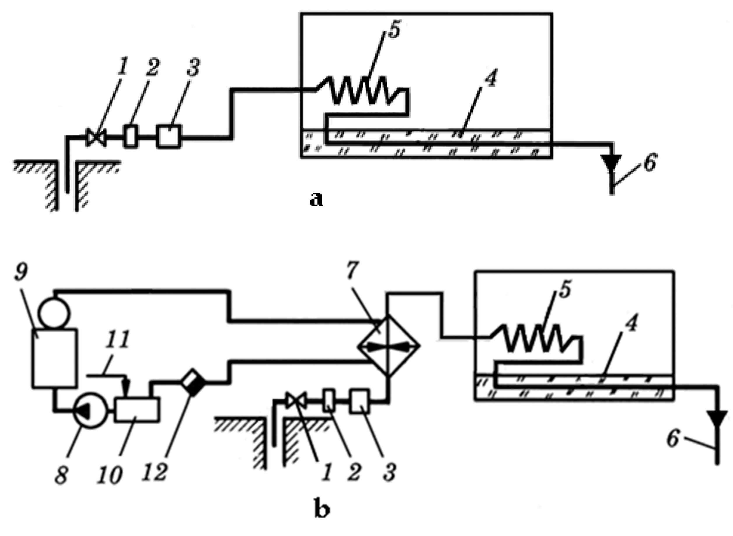
The following methods of using geothermal water are available for heating greenhouses [3]:

• direct water supply to the heating system (Figure 1a),
• direct water supply and special water treatment,
• direct water supply and heating in hot water boilers or heat exchangers (Figure 1b), and
• supply according to an independent scheme and the use of intermediate heat exchangers of the contact, surface, and contact-surface types (Figure 1c).

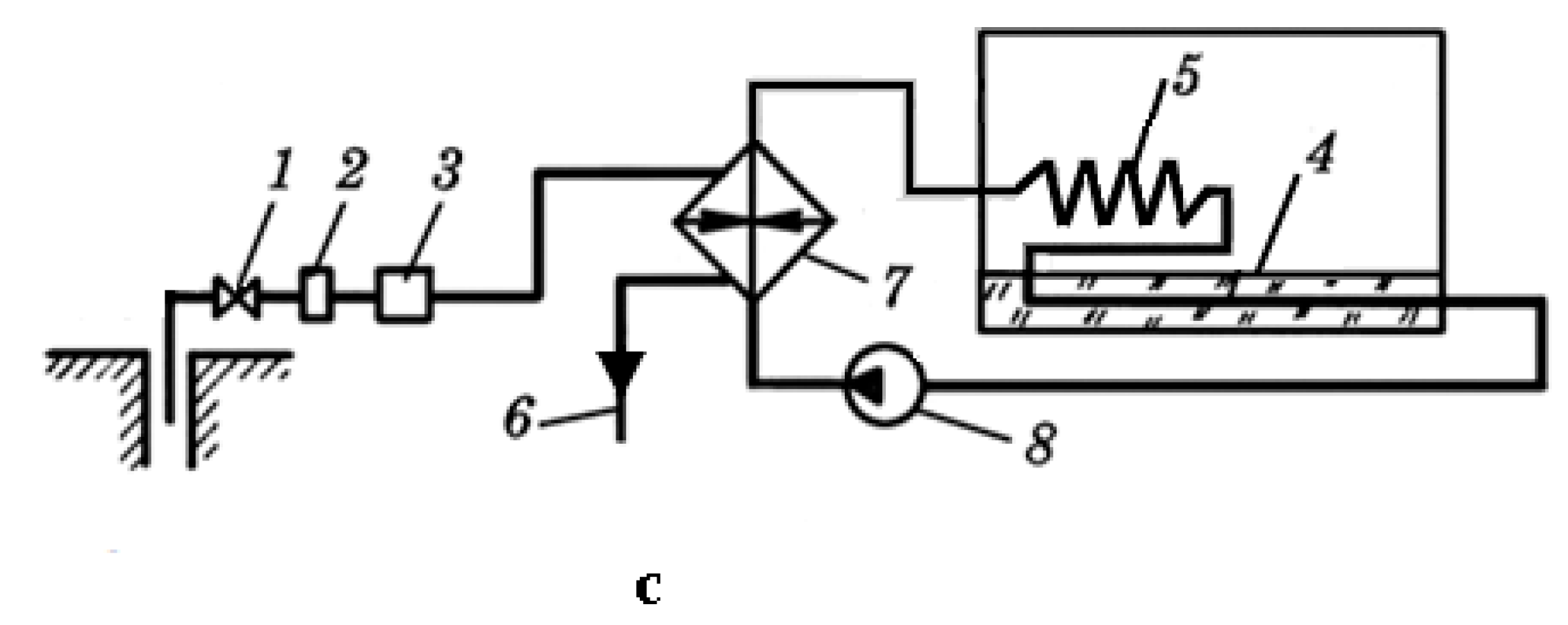
Figure 2 shows a functional diagram of a geothermal heating system for greenhouses with a surface heat exchanger.

The considered subsystem includes the following elements: a geothermal well, an electric ball valve, a mud sump, a degasser, a feed pump, and a heat exchanger. Water enters the sump and degasser. Then, pumps supply the water to the plate heat exchangers, where the heat carrier circulating directly in the heating circuit is heated. After the water passes through the heat exchangers, cooled geothermal water is discharged [1].

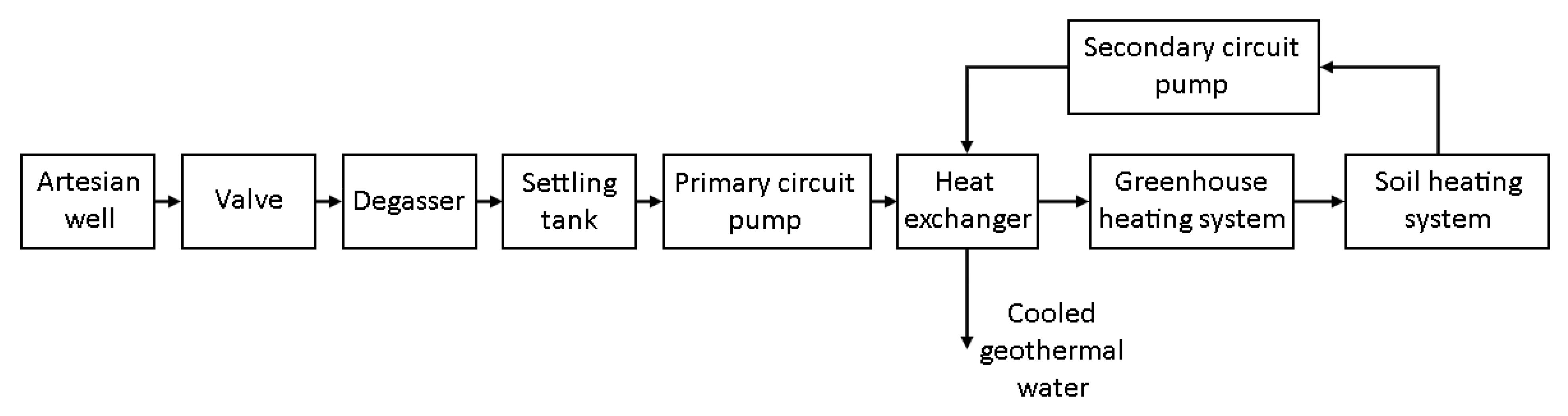
To ensure greater efficiency of the heat supply system, acoustic–magnetic devices were installed to prevent the formation of scale, which reduces the efficiency of the system. The functional diagram of the system using acoustic–magnetic devices is shown in Figure 3 [1].

For the practical application of AMDs, it is necessary to ensure that the ultrasonic transmitter operates within the certain temperature range. Even when the ambient temperature is stabilized, there is a heating of the transducer due to its own losses during the intensive oscillation mode. Measurements have revealed a heating of the ferrite core’s surface by 10–30 °C at an intensity of 3 W/sm² of sound emitted into the water. There are noticeable temperature gradients in the core. It is necessary to understand the dependence of the properties of ferrite transducers on the temperature. The temperature characteristics of ferrite cores may change during the operation of the device. The relationship between the temperature variations of magnetic permeability ${\mathsf{\mu }}_{\Delta }$ and the temperature variations of symmetrical hysteresis loop parameters ${\mathrm{B}}_{\mathrm{m}}$, ${\mathrm{B}}_{\mathrm{r}}$ and ${\mathrm{H}}_{\mathrm{c}}$ (${\mathrm{H}}_{\mathrm{m}}=10{\mathrm{H}}_{\mathrm{c}}$), induction difference $\Delta {\mathrm{B}}_{\mathrm{cv}}={\mathrm{B}}_{\mathrm{m}}-{\mathrm{B}}_{\mathrm{r}}$, absolute and relative variations of all these quantities were determined by the authors of [19].

Increasing the coercive force ${\mathrm{H}}_{\mathrm{c}}$ with a change in the temperature reduces the relative value ${\mathrm{H}}_{\mathrm{st}}/{\mathrm{H}}_{\mathrm{c}}$ of the magnetization field (${\mathrm{H}}_{\mathrm{st}}$—static magnetization field strength) and increases the temperature change of the magnetic permeability ${\mathsf{\mu }}_{\Delta }$. Decreasing the coercive force increases the relative value ${\mathrm{H}}_{\mathrm{st}}/{\mathrm{H}}_{\mathrm{c}}$ of the magnetization field but decreases the temperature change of the magnetic permeability ${\mathsf{\mu }}_{\Delta }$. A temperature change of the coercive force is not always the dominant factor influencing the change of magnetic permeability ${\mathsf{\mu }}_{\Delta }$. This value changes dramatically with the change in the magnetization field, for example, in the region of technical saturation. Changing a parameter of the symmetrical hysteresis loop rectangularity may influence the temperature change of the magnetic permeability as well. If the symmetrical hysteresis loop becomes more rectangular as the temperature changes, the magnetic permeability ${\mathsf{\mu }}_{\Delta }$ decreases. This corresponds well to the saturation region of almost all brands of ferrite.

The analysis of the relationship between temperature variations in the magnetic permeability ${\mathsf{\mu }}_{\Delta }$ and the parameters of the symmetrical hysteresis loop in the design of temperature-stable grades of pulse ferrites leads to the following conclusion: A material with a small change in coercive force and the rectangularity coefficient of the symmetrical hysteresis loop should be used in a given temperature range. In addition, the influence of temperature variations in these parameters on the changes in magnetic permeability ${\mathsf{\mu }}_{\Delta }$ should be mutually compensated. The temperature stability of the initial magnetic permeability does not guarantee the temperature stability of the partial-cycle permeability over a wide range of magnetic field induction values.

The study of characteristics of different-grade ferrite cores ${\mathsf{\mu }}_{\Delta }({\mathrm{H}}_{\mathrm{c}})$, $\Delta {\mathrm{B}}_{\mathrm{cv}}({\mathrm{H}}_{\mathrm{c}})$, ${\mathsf{\mu }}_{\Delta }(\Delta {\mathrm{B}}_{\mathrm{cv}})$, and ${\mathrm{H}}_{\mathrm{c}}(\Delta {\mathrm{B}}_{\mathrm{cv}})$ from a large number of batches showed that the temperature changes of this characteristic non-linearly depend on $\Delta {\mathrm{B}}_{\mathrm{cv}}$ and temperature. It is established, that at small values of magnetization field strength ([0;2,4] A/m) magnetic permeability ${\mathsf{\mu }}_{\Delta }$ and $\Delta {\mathrm{B}}_{\mathrm{cv}}$ at temperature +100 °C increase.

As explained by the authors of [20], at $\Delta {\mathrm{B}}_{\mathrm{cv}}$ = 14 T and a temperature of +100 °C, the ${\mathsf{\mu }}_{\Delta }$ change is −47%, and the ${\mathrm{H}}_{\mathrm{c}}$ change is +83%. At −60 °C, the ${\mathsf{\mu }}_{\Delta }$ change is +15%, and the ${\mathrm{H}}_{\mathrm{c}}$ change is −10%. On the one hand, the ${\mathrm{H}}_{\mathrm{c}}$ is inversely proportional to ${\mathsf{\mu }}_{\Delta }$, which determines the opposite signs of the temperature changes. On the other hand, ${\mathsf{\mu }}_{\Delta }$ and ${\mathrm{H}}_{\mathrm{c}}$ non-linearly depend on the induction drop, which determines the non-uniformity of the temperature variation’s absolute values. The sharp increase ${\mathrm{H}}_{\mathrm{c}}$ in the induction high decreases, and temperature of +100 °C is due to the transition to the saturated zone. The strength magnetization field increase at temperatures +100 °C can be explained by the fact that the slope of the $\Delta {\mathrm{B}}_{\mathrm{cv}}({\mathrm{H}}_{\mathrm{c}})$ dependence decreases in this case. After an investigation of the temperature characteristics of several (2000 HM1, 1500 HM3, 1000 HM3) ferrite cores from different brands, we found that the temperature variations of $\Delta {\mathrm{B}}_{\mathrm{cv}}({\mathrm{H}}_{\mathrm{c}})$, ${\mathsf{\mu }}_{\Delta }({\mathrm{H}}_{\mathrm{c}})$ and ${\mathrm{H}}_{\mathrm{c}}(\Delta {\mathrm{B}}_{\mathrm{cv}})$ dependences were significant greater than temperature variations of initial magnetic permeability. Due to the nonlinearity of ${\mathsf{\mu }}_{\Delta }({\mathrm{H}}_{\mathrm{c}})$ dependence, the temperature-stable ferrite grade for AMD operation can be used only if the temperature stability of such parameters of the symmetric hysteresis loop as a coercive force, residual, and maximum induction is obtained [20].

If the operating mode of the AMD is chosen with small values of the induction drop at the initial section of $\Delta {\mathrm{B}}_{\mathrm{cv}}({\mathrm{H}}_{\mathrm{c}})$ dependence, where the magnetic permeability ${\mathsf{\mu }}_{\Delta }$ of the partial cycle is at a maximum value (${\mathrm{H}}_{\mathrm{st}}/{\mathrm{H}}_{\mathrm{c}}$ is at a minimum value), then to transfer of the same pulse area with the AMD, a larger cross-section of the magnetic wire and a larger number of winding turns are required compared to the operating mode at the $\Delta {\mathrm{B}}_{\mathrm{cv}}({\mathrm{H}}_{\mathrm{c}})$ dependence saturation section. Increasing the magnetic wire cross-section and the number of winding turns, in addition to increasing the AMD dimensions, increases the parasite parameter values [20]. Operation in the $\Delta {\mathrm{B}}_{\mathrm{cv}}({\mathrm{H}}_{\mathrm{c}})$ dependence saturation region entails a sharp increase in the magnetization with a small increase in the induction drop. In this area, a small variation in the inductance differential, which may be related to, for example, main voltage variations, results in a sharp change in the magnetization current. In addition, when the core is heated and when the saturation induction drop decreases with the increasing temperature, the temperature changes in the magnetization field are so great (+200–300%) that the possibility of using the core in these modes is ruled out.

To solve the problems described above, a strategic simulation was proposed, as a simulation experiment provides more possibilities than a field experiment. In a simulation experiment, the distributions of random variables are at the experimenter’s disposal, whereas in a natural experiment, they are given by nature [21].

For the simulation, the quantities determining the process of scale prevention and the parameters of the acoustic–magnetic device (AMD) for a pipe with an external diameter of 75 mm were identified. The process of salt extraction from geothermal water treated by physical fields can be represented by a simplified relationship:

$$\mathsf{\xi }=\mathrm{F}(\mathrm{f},\mathrm{n},\mathrm{U},\mathrm{t},\mathrm{T})$$

(1)

where $\mathrm{U}$ is a three-phase rectangular voltage supplied to the acoustic–magnetic device (AMD), $\mathrm{f}$ is a voltage frequency supplied to the AMD, $\mathrm{n}$ is a number of winding turns of the AMD, t is a time during which three-phase rectangular voltage is supplied to the AMD, and T is a temperature of the AMD.

The supply pipe (diameter 159 mm) carries a large volume of water (90 m³/h) at a high pressure (4 at = 392,266 Pa). Therefore, we decided to make a bypass connection and install the AMD on it. For the bypass connection, a polypropylene pipe with an outside diameter of 75 mm and an inside diameter of 50 mm was used.

The calculation of the acoustic–magnetic device working area is the first step in the process of determining the parameters, as the installation of the device on the pipe is carried out by means of interference fit. It is known from theoretical sources [22] that the non-reagent water treatment process will be effective if at least one-third of the geothermal water flowing through the pipe is treated by physical fields.

Thus, we calculated basic data necessary for the construction of the model. In addition, we carried out the simulation for the pipe, which had an external diameter of ${\mathrm{D}}_{\mathrm{pd}}=75$ $\mathrm{mm}$ and an internal diameter of ${\mathrm{D}}_{\mathrm{Id}}=50$ $\mathrm{mm}$.

The velocity of the liquid in the pipeline was calculated using the formula:

$$\mathrm{V}=\frac{4{\mathrm{Q}}_{\mathrm{s}}}{\mathsf{\pi }{\mathrm{D}}_{\mathrm{Id}}}=0.41 (\mathrm{m}/\mathrm{s})$$

(2)

where ${\mathrm{Q}}_{\mathrm{s}}$ is the water flow rate per second (${\mathrm{Q}}_{\mathrm{s}}=0.00115$${\mathrm{m}}^3/s$).

The cross-sectional area of water in the working gap was calculated by the formula:

$${\mathrm{S}}_{\mathrm{wg}}=\frac{{\mathrm{Q}}_{\mathrm{s}}}{0.36\mathrm{V}\mathrm{m}}=0.41(\mathrm{m}/\mathrm{s})$$

(3)

where k is the number of operating gaps included in parallel.

The time of passage of fluid through the core of the AMD was $\mathsf{\tau }=0.296$ s.

The path length of fluid in the core of the AMD was:

$$\mathrm{L}=\mathrm{V}\mathsf{\tau }=0.12 \left(\mathrm{m}\right)$$

(4)

The external diameter of the pipe was the internal diameter of the AMD. The required diameter of the AMD should be 0.1 mm smaller than the inner diameter of the pipe for an interference fit. The inner diameter of the AMD housing was calculated according to the formula:

$${\mathrm{D}}_{\mathrm{idAMD}}=\frac{{\mathrm{S}}_{\mathrm{wg}}}{\mathsf{\pi }\mathrm{r}}+\mathrm{r}=0.07515 (\mathrm{m})$$

(5)

$${\mathrm{S}}_{\mathrm{p}}=\frac{\mathsf{\pi }{\mathrm{D}}^2{}_{\mathrm{pd}}}{4}=0.0044 ({\mathrm{m}}^2)$$

(6)

$$\mathrm{r}=0.5{\mathrm{D}}_{\mathrm{pd}}\sqrt{{\mathrm{D}}^2{}_{\mathrm{pd}}-\frac{4{\mathrm{S}}_{\mathrm{p}}}{\mathsf{\pi }}}=0.04 (\mathrm{m})$$

(7)

After selecting the internal diameter of the AMD, we calculated the operating frequency of the radiator based on the experimentally determined and model-calculated parameters. Then, we found the ferrite core with a 76 mm-greater internal diameter than the reference tables. The M2000HM ferrite ring (125 × 80 × 12 mm) satisfied these requirements. The resonant frequency of the selected ferrite ring was calculated according to the formula:

$$\mathrm{f}=\frac{\mathsf{\nu }}{2\mathsf{\pi }{\mathrm{R}}_{\mathrm{m}}}=\mathrm{14,782} (\mathrm{Hz})$$

(8)

$${\mathrm{R}}_{\mathrm{m}}=\frac{{\mathrm{R}}_{\mathrm{or}}+{\mathrm{R}}_{\mathrm{ir}}}{2}=\frac{0.0625+0.04}{2}=0.0513 (\mathrm{m})$$

(9)

where $\mathsf{\nu }=4760$ (m/s) is the velocity of the elastic vibrations in ferrite, ${\mathrm{R}}_{\mathrm{or}}$ is the external radius of the ferrite ring, ${\mathrm{R}}_{\mathrm{ir}}$ is the inner radius of the ferrite ring, and ${\mathrm{R}}_{\mathrm{m}}$ is the average radius of the ferrite ring.

Using the average diameter, we determined the active width of the transmitter ring $\mathrm{b}$. We experimentally determined that the optimum width $\mathrm{b}$ of the active part of the ferrite ring was 15–20% of the value of the average diameter of the ferrite ring ${\mathrm{D}}_{\mathrm{m}}$:

$$\mathrm{b}=(0.15÷0.2){\mathrm{D}}_{\mathrm{m}}=0.0205 (\mathrm{m})$$

(10)

The height of the selected ferrite ring was $0.012$ m, which was approximately the calculated value.

The geothermal water flow in the AMD working gap had a temperature of 56–78 °C. The external surface of the AMD was in the air, with temperatures between −10 °C and 15 °C and a convection coefficient of 3 W/K m. We assumed that the heat exchange is carried out with the thermal conduction and the convective movement of water and air. In the model, the water and air did not move, and the heat exchange was simulated by the mass transfer with an increased thermal conductivity of 50 W/K m. It was necessary to determine the time during which the voltage was supplied to the AMD until its temperature reached the value closest to the critical value (overheat temperature), as well as the time required for the cooling down of the AMD to an acceptable value while the volumes of the treated and untreated water in the heat supply system were at a ratio of 1:3.

To optimize the acoustic–magnetic effect, the parameters are were in a certain range. In particular, the AMD heating temperature did not exceed 67 °C, and the ratio of AMD runtime to AMD shutdown time was 1:3.

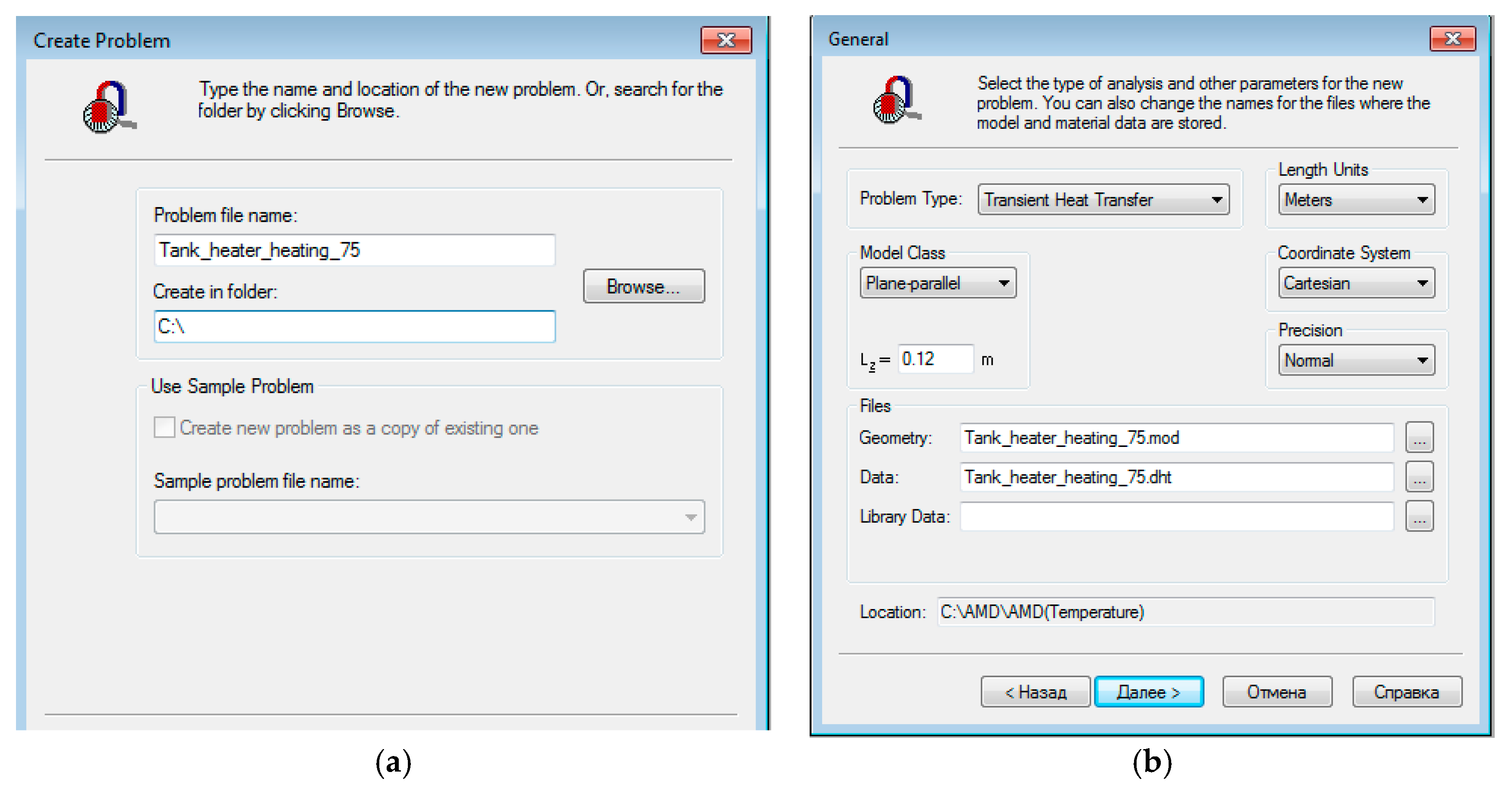
To solve this problem, the QuickField Student Edition environment was chosen. This environment allowed us to link the non-stationary thermal problems and to transfer the temperature distribution from one problem to another. The problems are based on a common geometric model file but can have different material property files and simulate different time intervals. It is possible to create a long-chain problem. In this way, sequential problem solving allowed us to stimulate a certain interval of the thermal process.

In the first step, the model was built in QuickField Student Edition to solve the problem. The non-stationary heat transfer problem was created with convection boundary conditions. The class of this model was the flat-parallel problem “First Heating Problem” (Figure 4).

Since this problem was non-stationary, it was necessary to specify the integration step and the finite time (

Table 1. Set-up of the integration over time of the new problem.

Timing	Time (s)	Temperature (°C)
Integration over Time Calculate up to	1800
With the step of	5
Output Store the results ever:	5
Starting from the moment:	0
Initial temperature:		56

).

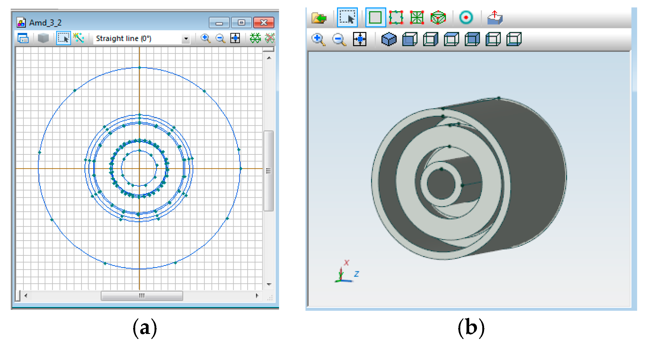
The initial temperature of the AMD was equal to the temperature of the pipe on which the AMD was installed (56 °C). The AMD overheat temperature should not exceed 67 °C ± 0.5 °C. The AMD model was presented in the Geometric Model Editor window (Figure 5).

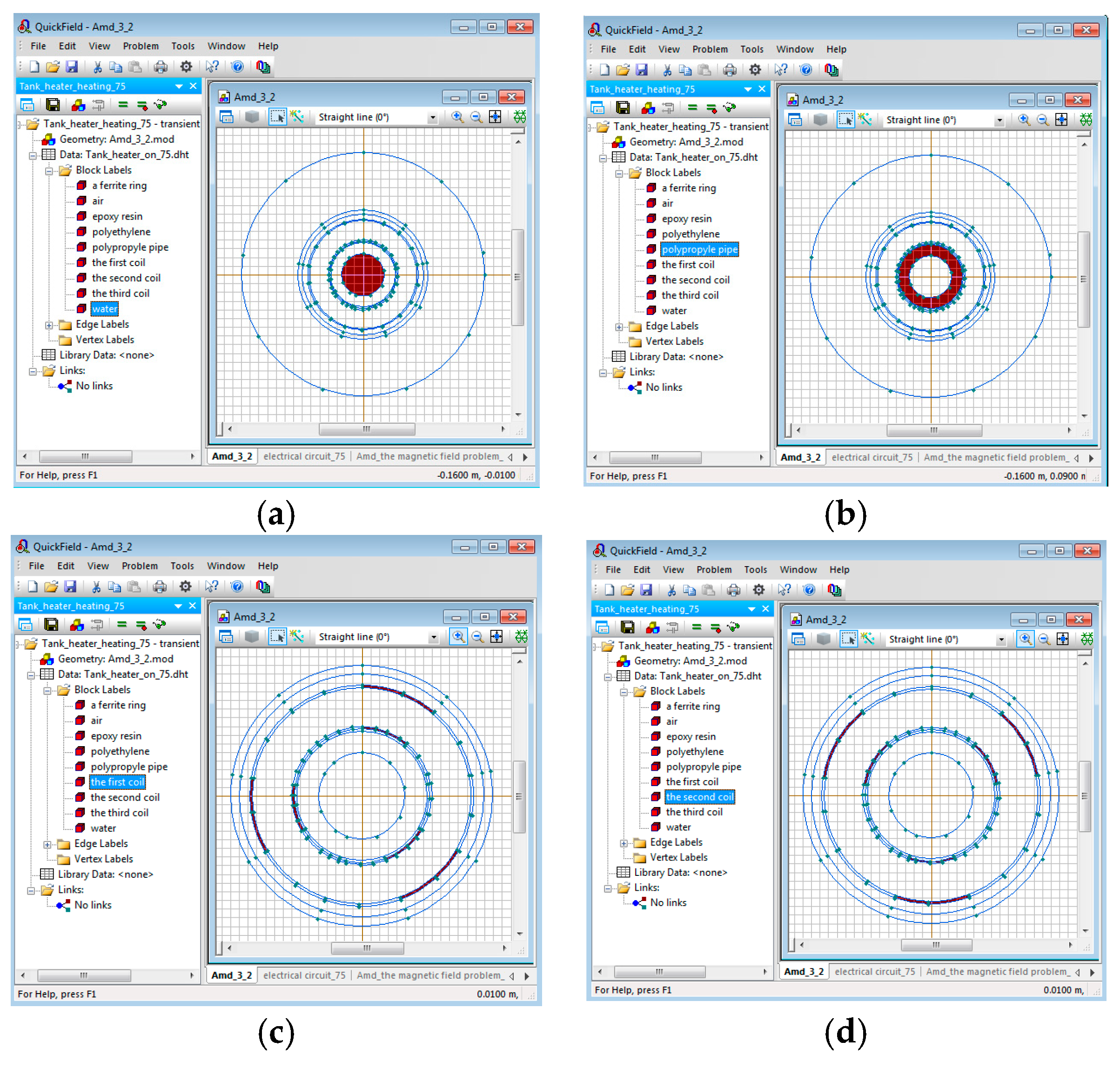
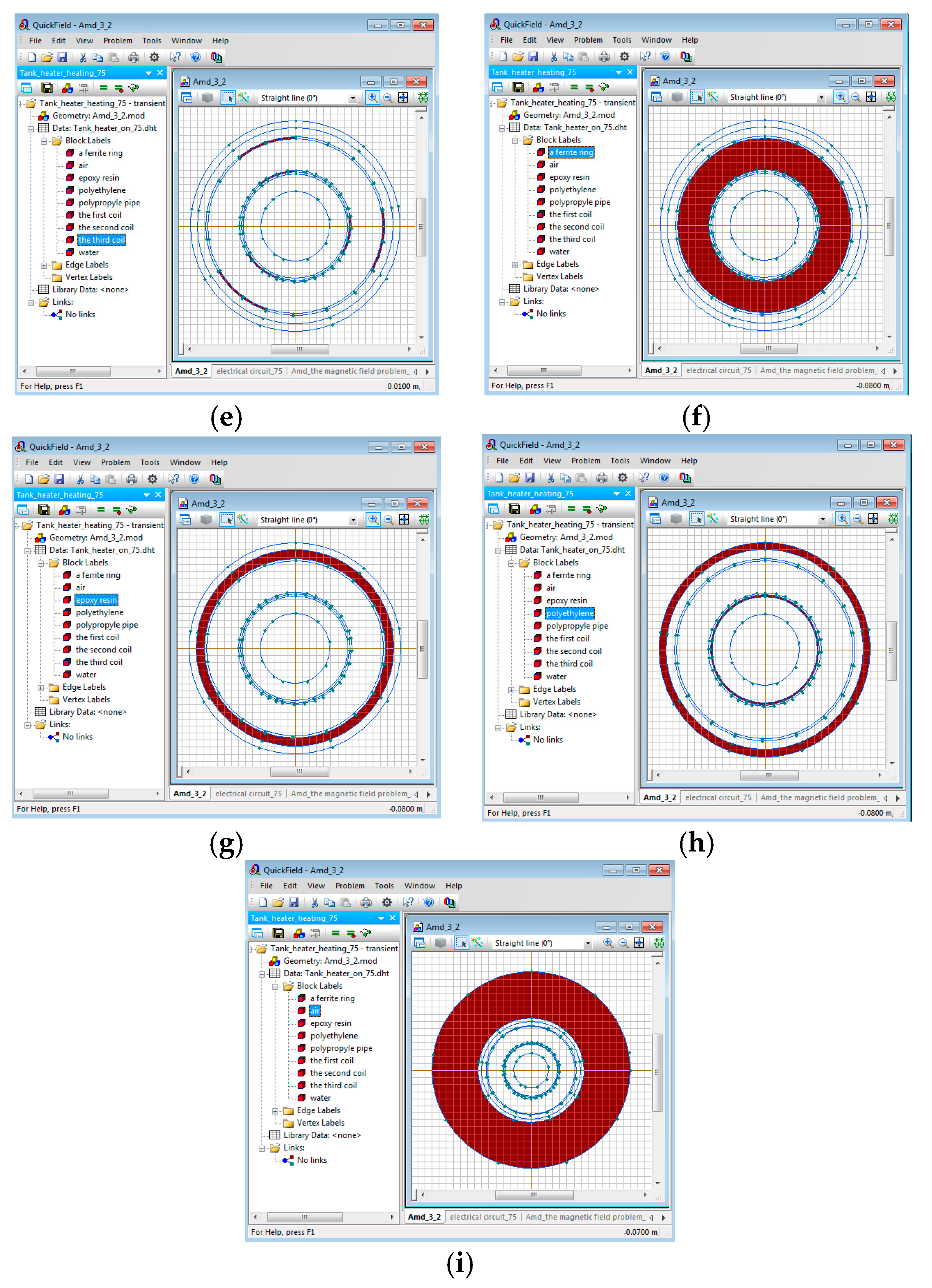
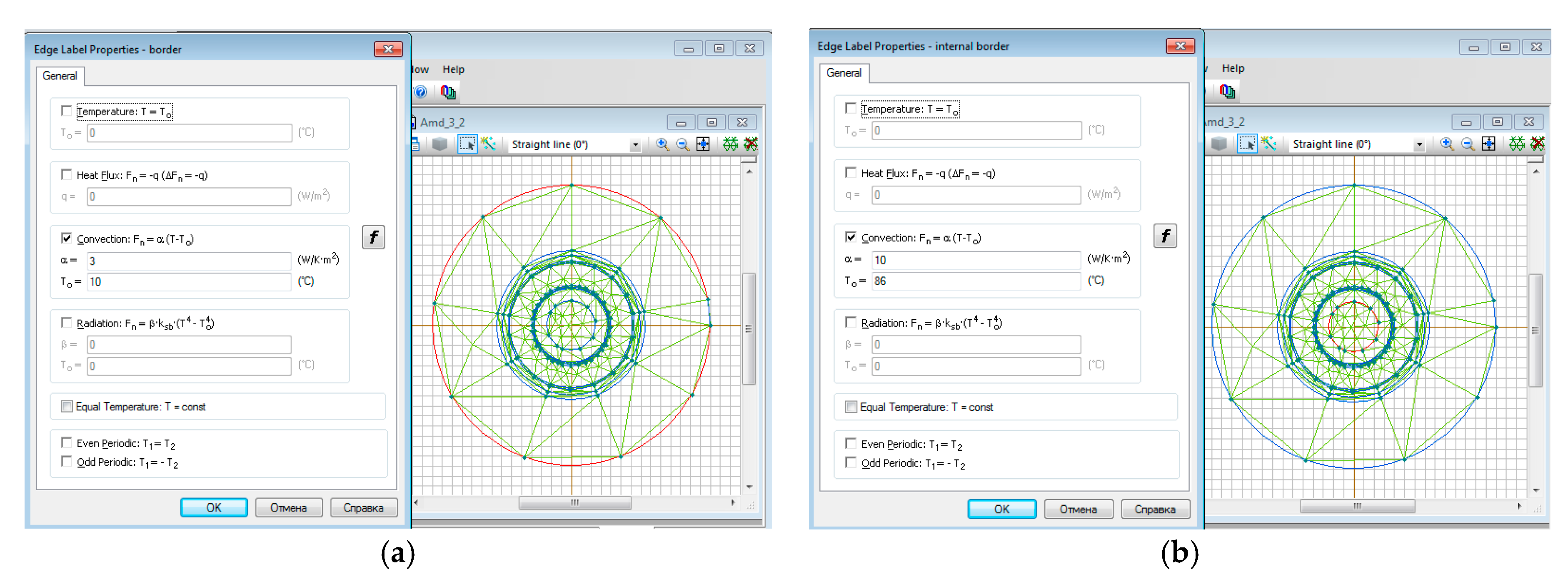
After designing the geometric model, we defined the labels and assigned physical properties to them. Figure 6 shows the correspondence of each given label to its geometric representation.

The surface was cooled by air. The convection coefficient was 3, and the ambient air temperature was 10 °C (Figure 7a). The temperature of the geothermal water inside the pipe was 86 °C. The convection coefficient was 10, and the temperature of the geothermal water was 86 °C (Figure 7b).

The physical properties of the labels are demonstrated in

Table 2. Physical properties of the labels.

Block Label Properties	Thermal Conductivity (W/K m)	Heat Capacity (J/kg K)	Density (kg/m3)	Volume Power of the Heat Source (W/m3)
“a polypropylene pipe”	0.2	1000	800	0
“air”	0.023	0	1.225	0
“a ferrite ring”	3.2	0	5270	0
“polyethylene”	0.4	1000	800	0
“water”	0.6	4200	1000	0
“epoxy resin”	0.4	1110	1200	0

.

The alternating current magnetic field problem must be solved to define the coil properties of all three phases. The heating power and the heating surface area must be determined to determine the volumetric heat dissipation density. The properties of labels of all three phase coils were set to calculate the heating surface area.

Table 3. Properties of the “the first coil” block.

Block Label Properties	Thermal Conductivity (W/K m)	Heat Capacity (J/kg K)	Density (kg/m3)	Volume Power of the Heat Source (W/m3)
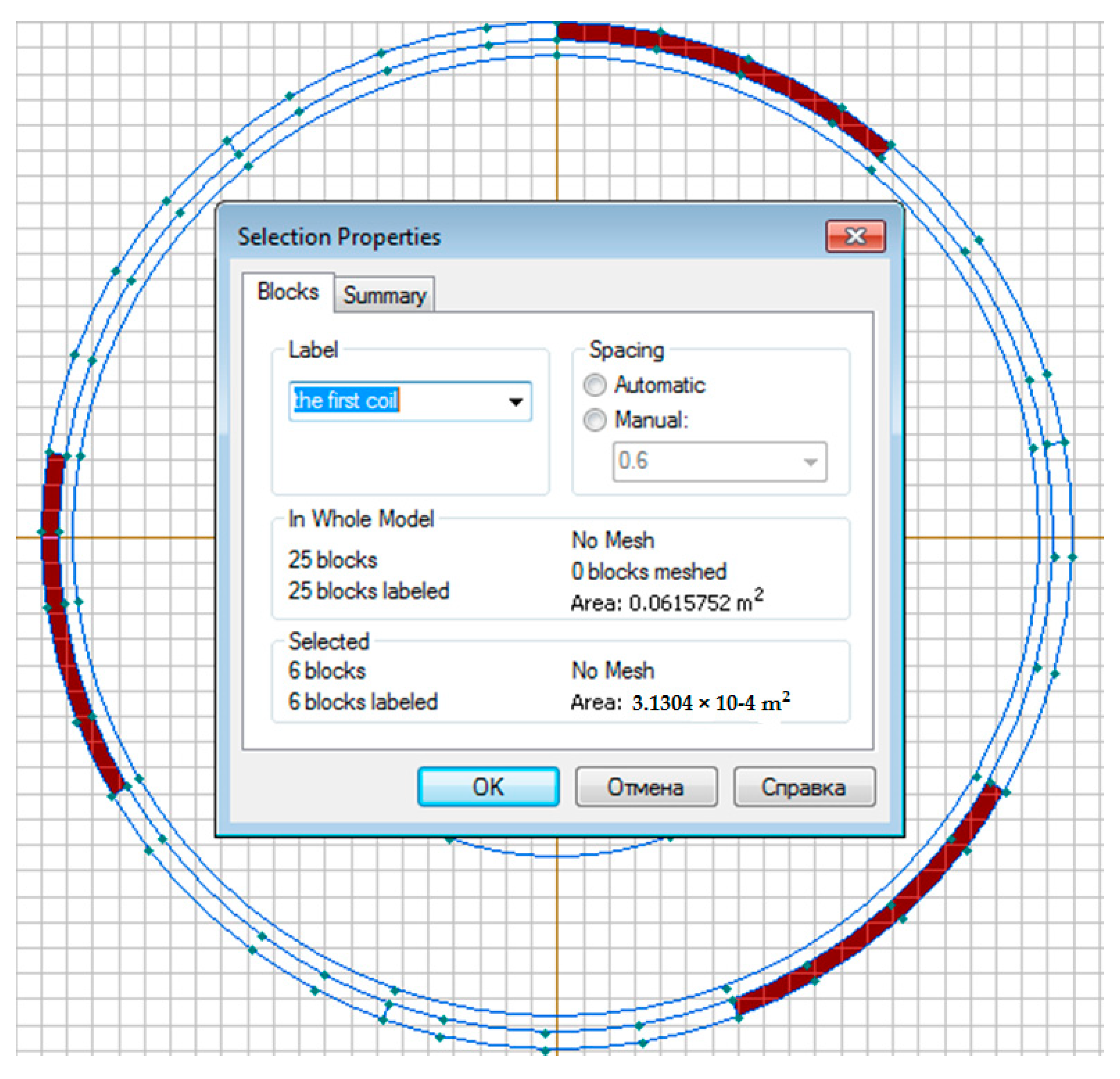
“the first coil”	380	100	8940	50/3.1304 × 10−4

shows the property of the label “the first coil”. The Figure 8 shows that the area was 3.1304 × 10⁻⁴ m².

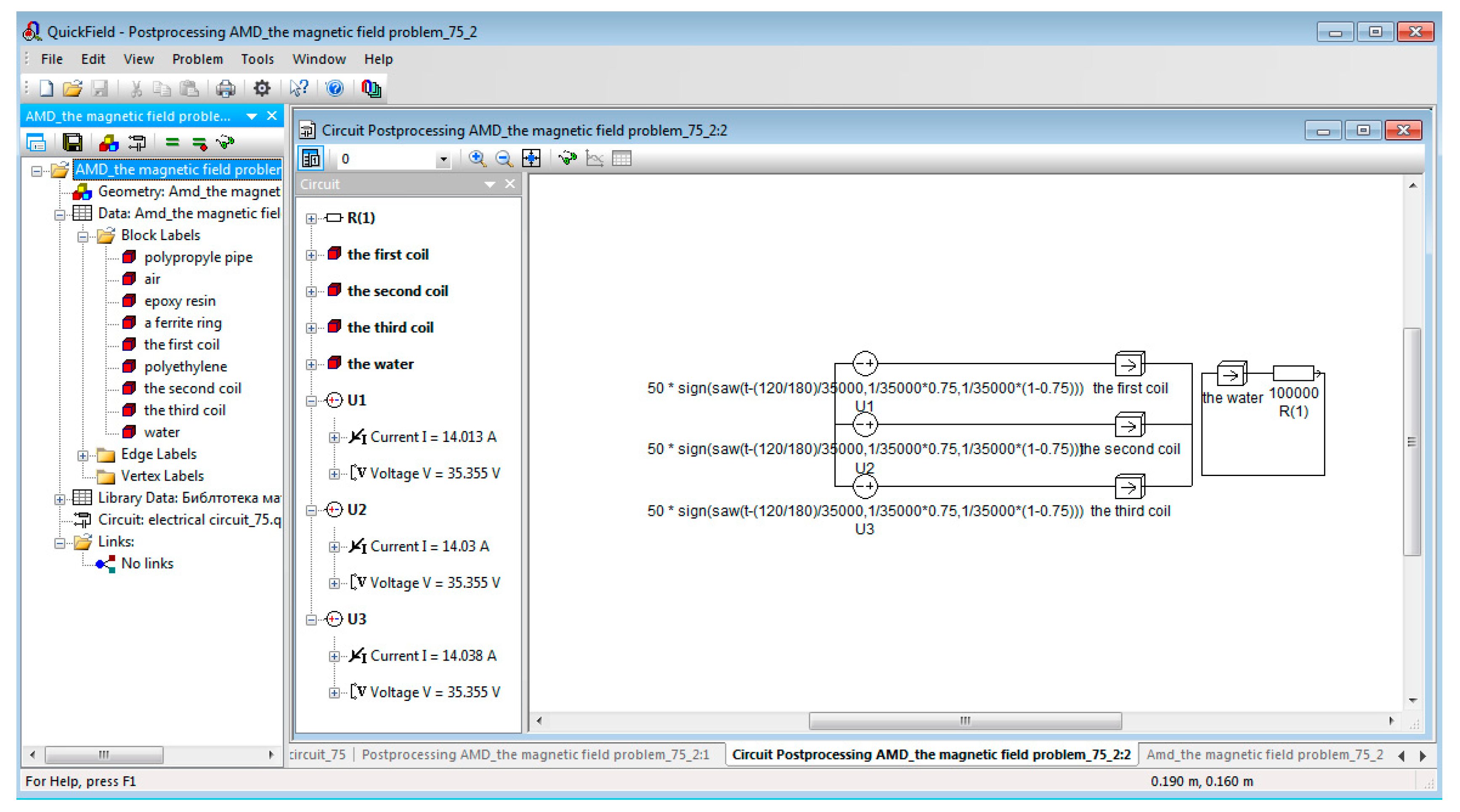
To calculate the power released when the AMD windings were heated, the AC magnetic field problem was solved. Figure 9 demonstrates the voltage and the current of the AMD windings. The current output of each coil was 50 W.

The properties of the blocks containing the windings of the three phases were specified. To specify the volumetric heat release area of the “the first coil”, we divided the found power by the volume. Table 3 shows the given properties of the “the first coil” block. The properties of the “the second coil” and “the third coil” were obtained in the same way.

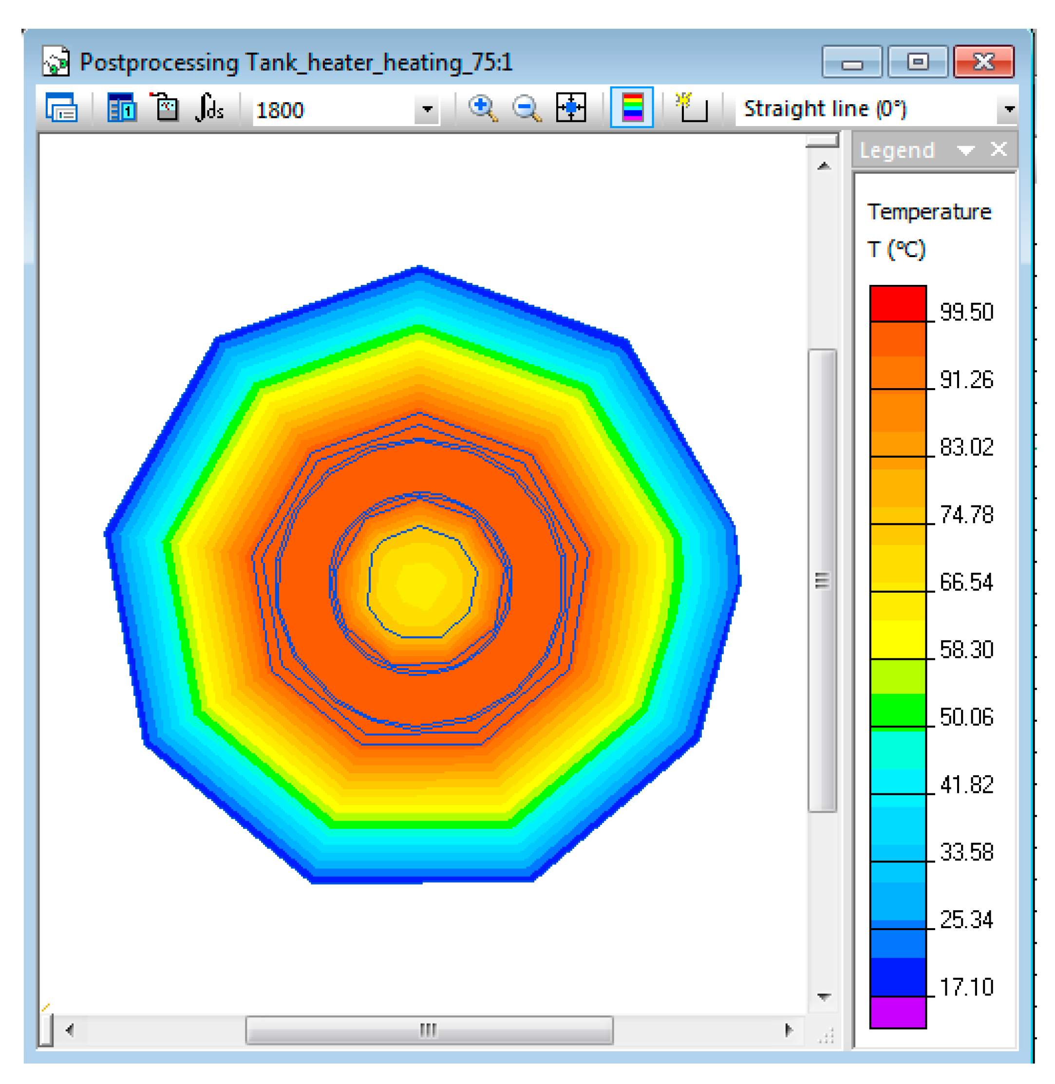
All steps to solve the problem were completed. Figure 10 demonstrates the AMD temperature distribution. The AMD temperature in the area of the ferrite ring exceeded 99 °C. Based on the initial conditions of the problem, the fact that the temperature exceeded the setpoints is significant. The graph demonstrates how the temperature of the ferrite ring changed over time.

The graph of the ferrite ring temperature variation for 1800 s is shown in Figure 11.

Figure 11 demonstrates that the temperature of the ferrite ring would reach 67 °C ± 0.5 °C after 300 s, which means that the heating of the AMD to the set value should not last more than 300 s. Therefore, we set the simulation time to 300 s.

Next, we solved the problem again. Then, the temperature did not exceed 67 °C. The AMD should be switched off after 300 s. To simulate the AMD cooling down process, it was necessary to solve a non-stationary heat transfer problem (“First cooling down problem”). We created a copy of the existing problem and imported the temperature distribution results of the already-solved problem to specify an initial temperature. Both problems must have the same geometric model file. We copied the properties of the first problem (“First heating problem”) to specify the properties of the labels of the second problem (“First cooling problem”). We needed to change the properties “volumetric heat emission” of the labels “the first coil”, “the second coil”, and “the third coil” by setting a value of 0, in order to set the AMD cooling conditions and simulate the AMD cooling process. It was necessary to connect the temperature value of the first and the second problems by selecting the heating problem file in the “task link” property, and set the start time of the problem to 300 s and the integration time to 1200 s. Figure 12 demonstrates the AMD cooling graph for 1200 s. The AMD cooled down to a temperature of 53.68 °C in 1200 s. The initial conditions set the external temperature of the pipe on which the AMD was mounted as 56 °C. Therefore, the AMD temperature cannot fall below this value. From the graph, it can be seen that the cooling time for 56 °C was equal to 854 s.

It was necessary to create a new non-stationary heat transfer problem (“Second heating problem”). We imported the temperature distribution of the already-solved cooling problem (“First cooling problem”) into a copy of the existing heating problem (“First heating problem”) to specify the initial temperature. For this purpose, both problems must have the same geometric model and data files. We set the time in the “Links” tab of the task properties to 854 s. In the “Naming” tab of the task properties, we set the time integration not exceeding the maximum heating time to 67 °C and performed the ratio of the treated and untreated water volumes as 1:3. For both conditions, the obtained dependencies in the solved problems (“First heating problem”, “First cooling problem”) should be approximated to a certain type of regression equation.

Table 4. Types of the regression dependence and their relative errors of approximation in the AMD heating process.

Types of Regression Dependence	Relative Error of Approximation	Regression Dependence
linear	0.29%	$\mathrm{y}=0.035\mathrm{x}+56.789$
exponential	0.38%	$\mathrm{y}={1.00057}^{\mathrm{x}}\times 56.89280$
power	2.26%	$\mathrm{y}=53.744{\mathrm{x}}^{0.030}$
hyperbolic	3.58%	$\mathrm{y}=6.4755/\mathrm{x}+62.2563$
semi-logarithmic	2.35%	$\mathrm{y}=4.2941\lg \mathrm{x}+53.4082$

and

Table 5. Types of regression dependence and their relative errors of approximation in the AMD cooling process.

Types of Regression Dependence	Relative Error of Approximation	Regression Dependence
linear	0.59%	$\mathrm{y}=-0.0122\mathrm{x}+65.9122$
exponential	0.48%	$\mathrm{y}={0.9998}^{\mathrm{x}}\times 66.0219$
power	2.68%	$\mathrm{y}=70.1549{\mathrm{x}}^{0.026}$
hyperbolic	3.79%	$\mathrm{y}=6.9245/\mathrm{x}+60.2284$
semi-logarithmic	2.59%	$\mathrm{y}=3.7775\lg \mathrm{x}+69.7645$

demonstrate that the relative error of approximation in the linear form of the regression dependence was minimal. This allowed us to set the similarity criterion for the AMD ferrite ring heating process (the “First heating problem”) in the form:

$${\mathsf{\pi }}_1=\frac{67.133-56}{300}=0.03711$$

(11)

For the cooling process of the AMD ferrite ring (the “First cooling down problem”), we set the similarity criterion in the form:

$${\mathsf{\pi }}_2=\frac{67.133-53.6298}{1200}=0.01125$$

(12)

Dividing ${\mathsf{\pi }}_2$ by ${\mathsf{\pi }}_1$, we obtain a similarity criterion. Using this criterion, we determined the interval during which the AMD temperature did not exceed 67 °C when the volume ratio of AMD-treated and untreated water was 1:3. The similarity coefficient has the form:

$${\mathsf{\pi }}_3=\frac{{\mathsf{\pi }}_2}{{\mathsf{\pi }}_3}=0.303$$

(13)

The integration time in the problem property in the “Naming” tab was set as:

$$300{\mathsf{\pi }}_3=91 (\mathrm{s})$$

(14)

The integration time in the properties of problem setting is the final step in the process of creating new problems. For the heating problem to use the temperature value from the cooling problem, it is necessary to link both problems by choosing “Links” in the task property of the cooling problem file (“First cooling down problem”) and to set the start time of the problem to 91 s. After that, we solved the problem. The graphical result of the problem solution is shown in Figure 13.

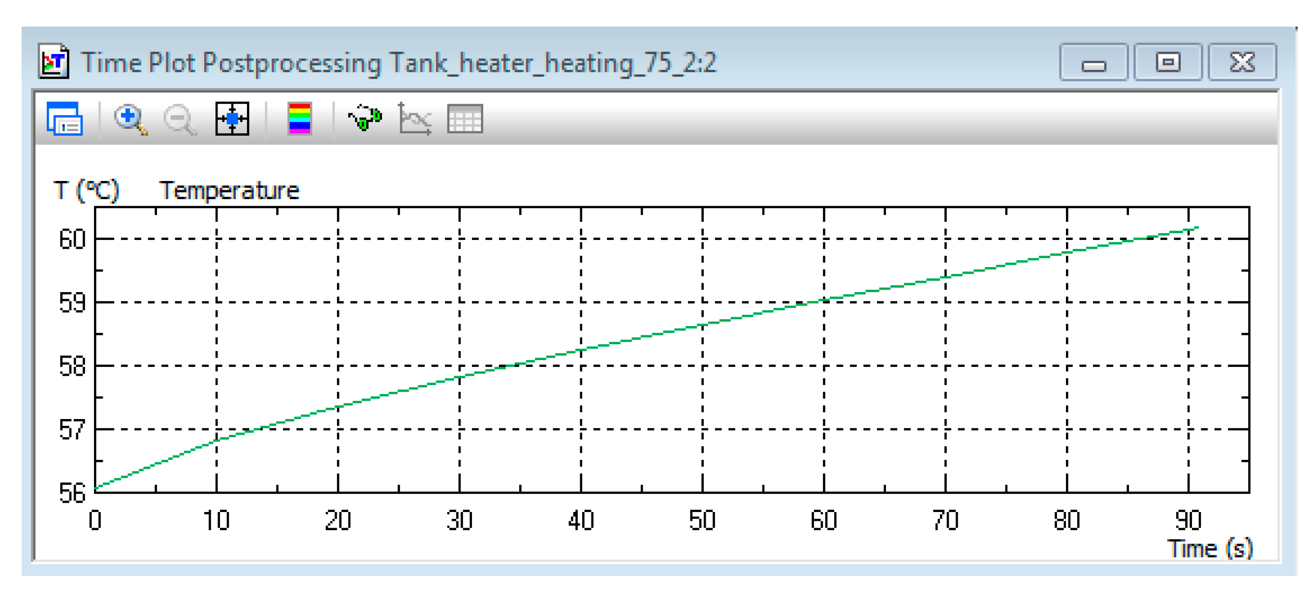
Figure 14 demonstrates that the average heating temperature of the ferrite ring by volume was 60.98 °C.

Next, we performed a simulation of the cooling process of the AMD. For this purpose, we created the new non-stationary thermal conductivity problem, which was a copy of the non-stationary thermal conductivity problem of cooling (“First cooling problem”). We call it the “Second cooling problem”. To create the cooling down problem, we used the temperature value from the previous heating problem (“Second heating problem”). The cooling down problem file (“Second cooling down problem”) was selected in the “Links” property of the problem, and the start time of problem solution was set to three-times the heating time (273 s). The problem solution was run. 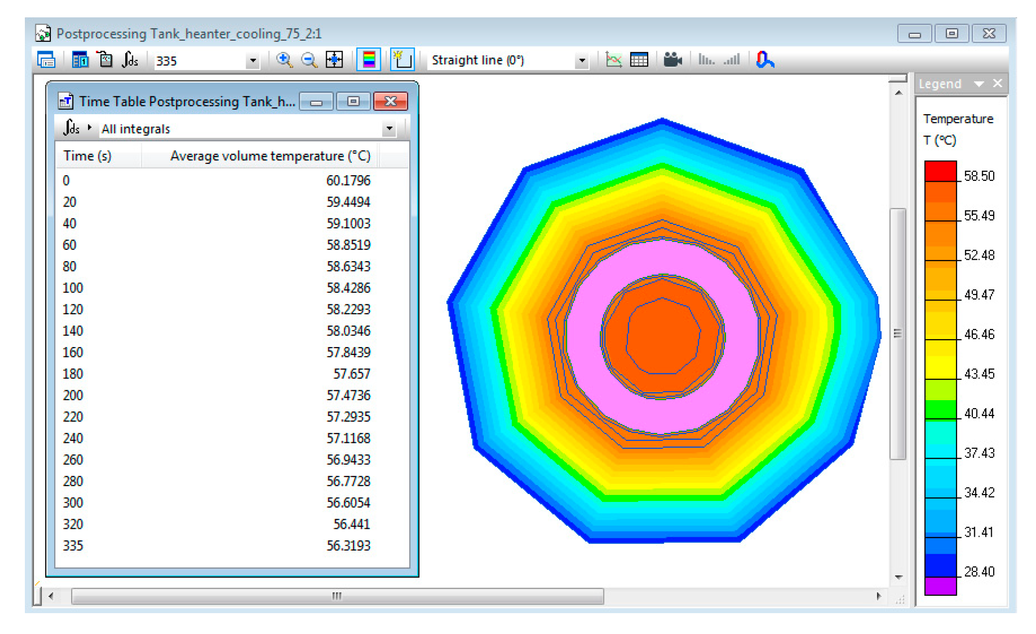Figure 15 shows the AMD cooling graph.

The final average cooling of volume temperature of the AMD ferrite ring was 56.83 °C. If we substituted this value into the regression equation of the AMD cooling (Table 5), we would obtain a value of approximately 61 s. It is possible to solve this problem if the integration time in the second cooling problem is set to 335 s. Figure 16 demonstrates the results of the simulation.

From the table (Figure 16), the “Average volume temperature” would have reached 56.32 °C in 335 s. This result indicates that the simulation achieved its goal. It is possible to keep the AMD temperature within the specified limits more accurately using the QuickField Student Edition open software interface and by creating a control system in LabVIEW. The control system would run the problems, measure the temperature at the end of the cycle, read the number of elapsed cycles (total process time), and include the data files. One data file would have zero source power, and the other would have nominal power. Thus, it would be possible to stimulate the heating or shutdown process by changing the reference to the data file.

3. Results

An acoustic–magnetic device enables a significant slowdown of the scale formation process on the internal surfaces of heat-exchange equipment in heat supply systems (for 9 months and more). This device has greater processing efficiency than other magnetic devices. For example, electrically driven valves have continued to operate faultlessly after 2 years [1].

In accordance with the results of previous research [1,23], we found that the processing efficiency of this device, in the case of its correct operation, reached 90%. These results are similar to those found with other magnetic water treatment devices, which have an efficiency of 40–45% [1,24,25,26].

Table 6. Parameters of reagent-free water treatment units.

Device	Conditional Diameters (mm)	Nominal Pressures (mPa)	Capacity of Processed Water (m3 h−1)	Magnetization Field Strength (kA m−1)	Consumed Power by the Electromagnet (kW)	Dimensions of the Magnet (mm)	Mass of Magnet (kg)
Magnetic device	80; 100; 200; 600	1.6	25–600	200	0.35–1.8	260 × 420; 440 × 835; 520 × 950; 755 × 1100	40; 200; 330; 1000
Acoustic–magnetic devices	80	4	25	0.015	0.1	-	1.2

presents the comparative characteristics of magnetic and acoustic–magnetic devices. The table shows that the characteristics of the acoustic–magnetic devices are much less energy-intensive than those of magnetic devices.

The effect on the crystallization centers of the acoustic and magnetic fields generated by the acoustic–magnetic device (Figure 17) [1].

Figure 17 demonstrates that untreated geothermal water, in contrast to the treatment with acoustic–magnetic device geothermal water, has obvious crystallization centers. Hence, we assume that acoustic–magnetic devices, acting on the crystals of salts, prevent their adsorption, thereby preventing the formation of solid deposits on the surfaces of the heat exchange equipment. The effectiveness of acoustic treatment is manifested in the prevention of the formation of primary crystals on the pipes [3].

The research carried out demonstrates the effectiveness of non-reagent treatment of geothermal water with an acoustic–magnetic device. The installation of these devices in the circuit of the geothermal heat supply system (Figure 18) led to a decrease in the frequency of system shutdown for unscheduled cleaning of the heat exchanger, which made it possible to reduce the labor intensity of manual operations of heat exchange equipment maintenance (removal of sludge, scale) and to reduce the economic costs of transportation and heat consumption [1,27,28].

To determine the effectiveness of the anti-scale effect, various methods are used. The most commonly used is the crystal-optical method [29], according to which the anti-scale effect θ is determined by the formula [1]:

$$\mathsf{\theta }=\frac{\mathrm{H}-\mathrm{M}}{\mathrm{H}}=\frac{0.0249-0.0029}{0.0249}$$

(15)

H—the dimension of solid deposits (inclusion) for untreated liquid, and

M—the dimension of solid deposits (inclusion) for treated with an acoustic–magnetic device liquid [1].

The values of the average linear sizes of salt crystals in treated and untreated water were calculated by an approximate calculation of the area of complex figures in relative unit measurements. The value of the anti-scaling effect is:

$$\mathsf{\theta }=0.88$$

(16)

After a long period of equipment exploitation, a small amount of scale was deposited, which was easily removed mechanically (Figure 19) [1].

The discrepancy between the experimental and the simulation values of AMD temperature (in the heat supply system with acoustic–magnetic devices) was estimated using the formula:

$$\mathrm{e}\mathrm{T}=\frac{{\mathrm{T}}_{\mathrm{sim}}-{\mathrm{T}}_{\exp }}{{\mathrm{T}}_{\mathrm{sim}}}100\%=2.3\%$$

(17)

where $\mathrm{e}\mathrm{T}$ is the calculated error of the ${\mathrm{T}}_{\mathrm{sim}}$, ${\mathrm{T}}_{\mathrm{sim}}$ is the simulated value, and ${\mathrm{T}}_{\exp }$ is the experimental value.

The discrepancy of the experimental and simulated data does not exceed 5%, which allows us to confirm the validity of the simulation and its fairly accurate correspondence to its physical prototype [3].

4. Discussion

The intensive formation of deposits on the internal surfaces of a heat supply system necessitates the replacement of the heating equipment before the end of the heating season, as well as the connection of back-up heat supply systems. Figure 20 demonstrates a section of a pipe from a geothermal heat supply system with deposits formed during the heating season. The problem is that scale formation takes the geothermal heating system out of operation.

Previous studies [30,31] have presented extensive research on various technologies and applications of geothermal energy. However, a comprehensive assessment of geothermal heating systems is relevant due to the changes in understanding the scope of application and evolution of technologies, which confirms the relevance of the research presented in the article [3].

Various models of acoustic–magnetic devices have been designed for geothermal water non-reagent treatment [32]. These devices have been tested at the geothermal deposits of the Maykop region of the Republic of Adygea. Our device for non-reagent acoustic–magnetic water treatment was used successfully at JSC “Raduga”. Acoustic–magnetic devices share the following characteristics: the amount of treated water is up to 0.25 m³/s, and the consumed power is about 50 W.

Research (2016–2020) of metal equipment protection from corrosion and salt deposition methods with geothermal water non-reagent treatment has a significant practical interest. The acoustic–magnetic geothermal water non-reagent treatment not only effectively protects the metal of the geothermal heat supply system equipment from corrosion, but also removes the existing deposits of salts and corrosion products in heat exchangers, pipes, and electric valves that disrupt their normal operation. The equipment downtime and cost of human labor and material resources for troubleshooting main heating systems and pipelines, which have been determined as a violation of the water-chemical regime, have decreased as a result. The problem of scale formation is solved by installing acoustic–magnetic devices that make it possible to automate the heat supply system of the greenhouse complex [3].

The simulation results are consistent with the data obtained from the installation of the acoustic–magnetic devices. It is necessary to fulfill several conditions to install the acoustic–magnetic device. The device will minimize the process of scale formation on the walls of the pipes and heating equipment. The main condition is that the device must be installed at the outlet of the geothermal well before the degassing system. The number of installed devices depends on the diameter of the supply pipe, water consumption, and type of acoustic–magnetic device. All devices must be connected in parallel to each other and with sludge traps. For high hourly water flows, to the device will process up to 30% of the solution flow. Before installing the acoustic–magnetic device, it is necessary to revise the entire geothermal water supply system; replace the pipelines and filters; and clean the old scale from the heat exchanger. Acoustic–magnetic devices and sludge separators are installed in such a way that they are always filled with geothermal water [3].

Figure 21 demonstrates the valve through which the geothermal water from the Maykop field flowed during the heating season when the geothermal water was treated with the acoustic–magnetic device.

5. Conclusions

In this paper, thermal protection technology of an acoustic–magnetic device was installed in the heat supply system of a greenhouse complex with a geothermal heat source. The acoustic–magnetic device was patented by the authors. To solve the set tasks, a strategic simulation was carried out a QuickField Student Edition v 6.4 simulation environment, which was suitable for this purpose. The simulation was carried out by installing the acoustic–magnetic device on pipes of various diameters, through which geothermal water flows from the geothermal wells with water of various temperatures. Thermal modes of the acoustic–magnetic device, as defined by the simulation, allow us to program the acoustic transducer of the acoustic–magnetic device at a resonance frequency that reduced the power inputs and increased the efficiency of the acoustic influence on the scale formed in the heat supply system of the greenhouse complex. The simulation results were implemented in the greenhouse complex of JSC “Raduga”. The thermal protection technology was realized by installing two acoustic–magnetic devices and automation systems in the geothermal heating system of the greenhouse complex. The optimal operating time of the acoustic–magnetic device allowed us to optimize the non-reagent treatment of geothermal water in the heating system of the greenhouse complex. Of the introduction of the acoustic–magnetic device thermal protection technology allowed us to significantly reduce the intensity of the scale formation in the heat exchanger and geothermal heating system equipment.