Article

Impact of Quadrature Booster on Power-System State Estimation in Polar Coordinates

Department of Electrical Power Engineering (K36), Wroclaw University of Science and Technology, Wybrzeze Wyspianskiego 27, 50-370 Wroclaw, Poland
*
Author to whom correspondence should be addressed.
Energies 2021, 14(18), 5992; https://doi.org/10.3390/en14185992
Submission received: 4 July 2021 / Revised: 6 September 2021 / Accepted: 13 September 2021 / Published: 21 September 2021

Abstract

:
The paper concerns the estimation of the state of a power system in which there is a phase shifter called a quadrature booster. The aim of the paper is a comparative analysis of two different cases including the quadrature booster in the state estimation. In the first case, the quadrature booster is represented by a model consisting of two real voltage sources, one in series with a power line and the other in a shunt branch. In the second case, in the power system model, the real branch with the quadrature booster is represented as off at the end where the considered quadrature booster is actually installed. The state estimation is assumed to be carried out in the polar coordinate system. The properties of the state estimation are characterized by: the number of iterations in the calculation process, the index of conditioning of the matrix of coefficients in the equations to be solved (cond(G)), and ratio Je/Jm, which is a measure of the accuracy of the estimation. Using IEEE 14-bus test system, investigations are carried out in such a way as to cover the entire state space of the power system as possible. In the investigations, Monte Carlo experiments are carried out for each of the considered cases of the state estimation. Each of these cases is also analyzed from the point of view of the assumed definition of the state estimation. Investigations show that in the first of the previously described cases, the state estimation is more accurate, but there are more iterations in the calculations and worse conditioning of the estimation process. The comparative analysis also shows that, the accuracy of the results obtained in each of the considered cases is practically independent of the coordinate system in which the estimation calculations are performed. Taking into account the number of iterations in the estimation process and index cond(G), it can be concluded that the implementation of each of the above-mentioned estimation cases in the rectangular coordinate system is more reasonable.

1. Introduction

1.1. Considered Problem and the Current State of the Research Field

Knowing the state of the power system is essential to be able to influence effectively the system. State estimation, which allows us to estimate the power system state on the basis of the possessed measurement data and the knowledge of the system topology [1], should ensure acceptable accuracy of determining this state. One of the important factors influencing that accuracy is the system model, which is used in state estimation. The system model consists of models of individual system components.
The paper considers the estimation of the state of the power system in which there is a phase shifter, being one of the FACTS controllers [2]. The phase shifter, causing a change in the phase shift between the voltages at the ends of a power line, enables a change in power flows on this line, as well as a change in power flows in a power system. In the paper, one of the types of phase shifters [3] is considered, namely the quadrature boosting transformer, also known as quadrature booster [4].
When there is a phase shifter in the power system, from the point of view of the state estimation the question arises: “How should this phase shifter be considered in the state estimation?” The presented question can be reduced to the following questions: “Can the state estimation procedure, which was developed for a power system without a phase shifter, be used to estimate the state of the system when there is a phase shifter in it?”, “If the phase shifter is to be included in the state estimation, what model should be taken into account?”.
One can find papers describing the estimation of the state of a power system with the phase shifter installed. In existing papers, phase shifters are considered at different levels of detail. In some papers, the phase shifter is considered generally, in other papers the phase shifter is considered after taking into account its type. In this paper, if it matters the type of the phase shifter will be given.
The inclusion of the phase shifter in the power system model, which is used in the state estimation, shown in [5], assumes that the phase shifter is represented with the use of two transformers. One of them is connected in series, the other—in parallel. The same method of the phase shifter modeling is taken into account in [6]. In [7], the authors state that when the phase shifter is installed in series with the power line between nodes i and j at node i, it is enough to insert δi + Δδi instead of the phase angle δi into measurement equations of such quantities as Pij, Qij, Pji, Qji, Pi, Qi, Pj, and Qj, where δi is a phase angle of nodal voltage V ¯ i ; V ¯ i is a voltage at node i; Pxy and Qxy are, respectively, an active and reactive power flow on the power line between nodes x and y at node x; x, y ∈ {i, j} and xy; and Px and Qx are, respectively, an active and reactive nodal power at node x.
In [8], state estimation, in which the phase shifter is modelled with the use of so-called the power injection model, is considered. In the case of that model, the effect of the presence of the phase shifter is treated as equivalent to the input of injection of the complex power at the relevant nodes (between them there is a power line and the phase shifter).
An admittance in series with an ideal transformer having a complex turns ratio represent the phase shifter in the power-system state estimation, which is considered in [9]. Paper [10] describes the power system state estimation assuming the use of a phase shifter model consisting of an ideal series voltage source and an ideal shunt current source. The use of two real voltage sources, i.e., a serial source and a shunt source in the phase shifter model for the state estimation purposes is described in [11,12,13,14,15]. Papers [11,12,13] deal with the state estimation for a power system with a quadrature booster. In [14,15], a power system with the symmetrical phase shifter is considered.
In [5,6,7,9,10] nothing is said about the quantitative assessment of the influence of the phase shifter on state estimation. Such an assessment is carried out in papers [8,11,12,13,14,15]. In [12,13,15], the properties of the estimation are examined when complete information about the phase shifter is included in it, i.e., information that also includes information about the type of the phase shifter.
Papers [11,12] consider the state estimation in the rectangular coordinate system. In [11], the properties of the state estimation for a system with a phase shifter are compared with the properties of the state estimation for a system without the phase shifter. When a phase shifter is included in the power-system model, the complexity of the model increases. It can therefore be predicted that under these conditions the power-system state estimation will have worse properties than the estimation of the state of the system without the phase shifter. However, it is important how big the differences are, so whether it is rational to look for more favorable state-estimation solutions for a system with the phase shifter. The research results, which are presented in [11], indicate that the previously mentioned differences should be considered significant.
In paper [12,13], the influence of the use of specific information about the quadrature booster in state estimation on the results of this estimation is investigated. In paper [12], the state estimation in the rectangular coordinate system and in [13] the state estimation in the polar coordinate system is considered. The research results show that the aforementioned effect is noticeable. As a result of the use of specific information about the quadrature booster, the accuracy of the results of the state estimation increases, and the conditioning of the computational process is improved and in the case of the state estimation in the polar coordinate system also the number of iterations decreases.
In the paper [14], the properties of state estimation in the rectangular and polar coordinate systems are investigated, taking into account the presence of a symmetrical phase-shifter in the power system, compared to the properties of the state estimation of the power system in which there is no phase-shifter. Research shows that in the former case, the state estimation properties are worse. From the point of view of the number of iterations and the conditionality of the computational process, the properties of estimation of the state of the power system in which there is a phase-shifter are more advantageous in the rectangular coordinate system than in the polar coordinate system. On average, the accuracy of the state-estimation results in both coordinate systems is comparable. The influence of the use of specific information about the symmetrical phase-shifter in state estimation in the polar coordinate systems on properties of this estimation is investigated in [15]. The use of the mentioned specific information in the state estimation increases the accuracy of the estimation results, significantly improves the conditionality of the computational process, but also significantly increases the number of iterations in the calculations.

1.2. Purpose of the Paper

The paper presents a continuation of the research carried out by the authors of the paper in the field of assessing the properties of estimation of the state of the power system, in which there is a phase shifter, for different ways of including the phase shifter in the estimation.
The paper presents the results of original comparative investigation of two methods of power-system state estimation. Analysis of the properties of the estimation of states of the power system, in which there is a quadrature booster, is made for each of the considered methods. Those methods are as follows:
  • Method 1—iterative estimation process is realized with the use of knowledge of the quadrature booster model, which consists of two real voltage sources, as it is in [11,12,13,14,15].
  • Method 2—iterative estimation process assumes that in the system model there is a switching off of the branch at the end of which there is the quadrature booster in the real system, and the switching off of the branch is at this end, where there is the quadrature booster.
In Method 2, no the quadrature booster model is introduced into the system model used in iterative estimation process.
In both considered methods, the state estimation is in the polar coordinate system. For each of these methods, the results of comparing the state-estimation properties in different coordinate systems are also shown.
Method 2 can be applied using an estimation program developed for a power system without the quadrature booster.
The state estimation proposal using method 2 is original. There are no papers in which such a state estimation would be considered.

1.3. Organization of the Paper

The paper consists of six sections and two appendices. In Section 2, a model of a quadrature booster is presented. In Section 3, a mathematical description of a power-system state estimation in polar coordinate system is given. This section also presents the characteristics of the two investigated methods of estimating the state of the power system, in which a quadrature booster is installed. Section 4 presents the results of comparative investigations of the considered estimation methods in the polar coordinate system from the point of view of the accuracy of results, sensitivity to measurement errors and their realization time. Part of the investigation concerns the properties of the considered methods in various coordinate systems. Section 5 is devoted to discussion. In Section 6, there are conclusions. The appendices contain the derivation of the formulas introduced in the paper.

2. A Model of the Quadrature Booster

A general equivalent circuit of a phase shifter is shown in Figure 1 [16]. In the equivalent circuit, there are two transformers: a shunt Excitation Transformer (ET) and a series Boosting Transformer (BT). Transformer BT injects a series voltage ( V ¯ BT ) in a power system. The phasor of voltage V ¯ BT is controlled by the tap changer.
A quadrature booster is one of types of the phase shifter. In the case of the quadrature booster, the phase shift between voltage V ¯ BT and voltage V ¯ i (see Figure 1) is equal only to −90° or 90° (Figure 2).
During consideration to be presented in the paper, the quadrature booster is represented by the model shown in Figure 3. The model consists of two controllable voltage sources. Their internal impedances z ¯ ET and z ¯ BT represent impedances of transformers ET and BT, respectively.
For the assumed model, the following equations can be derived:
S ¯ i l * = V i 2 y ¯ ET + y ¯ BT + V ¯ l V ¯ i y ¯ BT V ¯ BT V ¯ i y ¯ BT + V ¯ ET V ¯ i y ¯ ET ,
S ¯ l i * = V l 2 y ¯ BT + V ¯ i V ¯ l y ¯ BT + V ¯ BT V ¯ l y ¯ BT ,
S ¯ BT * = V BT 2 y ¯ BT + V ¯ i V ¯ BT y ¯ BT V ¯ l V ¯ BT y ¯ BT ,
S ¯ ET * = V ET 2 y ¯ ET V ¯ i V ¯ ET y ¯ ET ,
where: the designations of variables in the formulas refer to Figure 3; Vi and Vl are the magnitudes of voltages V ¯ i and V ¯ l , respectively; y ¯ ET = 1 / z ¯ ET , y ¯ BT = 1 / z ¯ BT , VET, and VBT are the magnitudes of voltages V ¯ ET and V ¯ BT , respectively.
In estimation procedure, powers S ¯ i l and S ¯ l i are used in power balance equations for nodes i and l.
The phase shifter does not absorb and inject complex power, and therefore:
S ¯ ET + S ¯ BT = 0 ,
where: S ¯ ET and S ¯ BT are the complex powers associated with the sources in the shunt and serial branches of the phase shifter model, respectively.
It will further be assumed that
S ¯ BB = P BB + j Q BB = S ¯ ET + S ¯ BT ,
where: P BB and Q BB are a real and imaginary part of S ¯ BB .
For the quadrature booster the following formula can be taken into account:
δ BT δ i δ BT tar = 0 ,
where: δ BT and δ i are phase angles of V ¯ BT and V ¯ i , respectively; δ BT tar is a target phase shift between vectors of voltages V ¯ BT and V ¯ i .

3. Background for the State Estimation

3.1. The Classical State Estimation

In this paper, the term of “the classical state estimation” is understood as a state estimation for a power system without a quadrature booster.
In the paper, the weighted-least-squares power-system state-estimation method is considered [17]. For that method, an objective function is following:
J x = 1 2 z h ( x ) T R 1 z h ( x ) ,
where: x is a power-system state vector; z is a vector of measurements; h(x) is a vector of functions of vector x, representing dependence of measured quantities on the state vector; and R is a diagonal matrix of measurement-data covariances.
State vector x in polar coordinate system is defined as:
x = δ 2 , δ 3 , , δ n , V 1 , V 2 ,   , V n T ,
where: δi i = 2, 3, …, n are phase angles of voltages at nodes 2, 3, …, n; Vi i = 1, 2, …, n are magnitudes of voltages at nodes 1, 2, …, n; and n is a number of all nodes in a power system.
Node 1 is considered as a reference node. The phase angle for that node is equal to zero.
The number of state-vector elements (nx) is as follows:
n x = 2 n 1 .
The relationships among measured quantities and elements of the state vector are as follows [18]:
V i = V i ,
P i j Q i = V ¯ i * Y r o w i V ,
P i j j Q i j = y ¯ s i + y ¯ i j y ¯ i j V i 2 V ¯ j V ¯ i * T ,
where: Pi and Qi are an active and reactive power injections at i-th node, respectively; Pij Qij are an active and reactive power flows, respectively, between i-th and j-th node, measured at i-th node; y ¯ i j is an admittance of the series branch connecting i-th and j-th node; y ¯ s i is an admittance of the shunt branch at i-th node; and Yrow i is the i-th row of an admittance matrix for the considered system:
Y r o w i = Y ¯ i 1 , Y ¯ i 2 , Y ¯ i n ,
Y ¯ i l i, l = 1, 2, …, n are elements of the admittance matrix and V is a vector:
V = V ¯ 1 , V ¯ 2 , V ¯ n T .
The relationships (11)–(13) are used for definition of elements of function vector h(x). Vector h(x) can be presented as follows:
h x = P AC _ 1 , , P AC _ n , Q AC _ 1 , , Q AC _ n , P f _ 1 , , P f _ 2 g , Q f _ 1 , , Q f _ 2 g ,   V 1 , , V n T .
Formula (16) assumes that: PAC_i = Pi, QAC_i = Qi i ∈ {1, 2, …, n}; Pf_j and Qf_j are, respectively, an active and reactive power flow at the end of the appropriate branch, j ∈ {1, 2, …, 2g}; and g is a number of all branches in a power system. The power flows are numbered according to the adopted rule.
The number of elements of vector h(x) (mz) is as follows:
m z = m + m z _ 0 ,
where: m is the number of measured quantities (the number of measurement data) and mz_0 is the number of quantities, of which values are known (the number of pseudo-measurements).
A pseudo-measurement is treated as a measurement of high accuracy. We assume that mz_0 is calculated using the formula:
m z _ 0 = 2 n 0 ,
where: n0 is the number of zero-injection nodes.
Note, for the zero-injection node, there are two pseudo-measurements, i.e., an active and reactive power flow. Each of those power is equal to zero.
The vector defined in Formula (16) has the maximal possible number of elements. That number is equal to 3n + 4g. In fact, often the number of elements of the vector h(x) is smaller because not all nodal powers, power flows as well as nodal voltage magnitudes are measured, or if they are measured they are not available.
The characterized estimation method assumes iteratively searching for a solution to the state-estimation problem. During this computational process, the normal-equation set is solved:
G x k x k + 1 x k = g ( x k ) ,
where: k is a number of iteration and xk is a solution of the state vector at k-th iteration,
G x k = H T x k R 1 H x k ,   H x = h x x ,   g ( x ) = J x x = H T ( x ) R 1 z h ( x ) .
G(x) is called a gain matrix.
Jacobian matrix H(x) can be presented as follows:
H ( x ) = P AC _ 1 δ 2 P AC _ 1 δ n P AC _ 1 V 1 P AC _ 1 V n P AC _ n δ 2 P AC _ n δ n P AC _ n V 1 P AC _ n V n Q AC _ 1 δ 2 Q AC _ 1 δ n Q AC _ 1 V 1 Q AC _ 1 V n Q AC _ n δ 2 Q AC _ n δ n Q AC _ n V 1 Q AC _ n V n P f _ 1 δ 2 P f _ 1 δ n P f _ 1 V 1 P f _ 1 V n P f _ 2 g δ 2 P f _ 2 g δ n P f _ 2 g V 1 P f _ 2 g V n Q f _ 1 δ 2 Q f _ 1 δ n Q f _ 1 V 1 Q f _ 1 V n Q f _ 2 g δ 2 Q f _ 2 g δ n Q f _ 2 g V 1 Q f _ 2 g V n 0 0 1 0 0 0 0 1
Matrix H(x) (like vector h(x) before) is presented under the assumption of the maximum number of measured quantities. When the number of these quantities is smaller, the number of rows of the vector h(x) and also of the matrix H(x) is smaller than previously assumed.
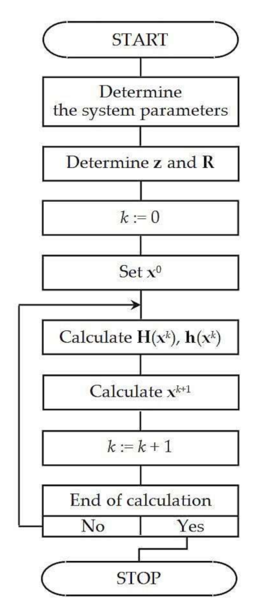
We can formulate the following algorithm for the considered case of the state estimation:
  • Determine the parameters of the power system elements.
  • Determine measurement vector z and measurement-data covariance matrix R.
  • Set vector x0, i.e., a vector whose elements are the initial values of the elements of state vector x.
  • k = 0.
  • Calculate elements of Jacobian matrix H(x) and vector h(x) for xk.
  • Calculate xk + 1, i.e., new approximation of vector x using (19).
  • k = k + 1.
  • If stopping criteria are fulfilled, calculate unmeasured quantities, else go to step 5.
A flow chart of the state estimation process is in Figure 4.
The necessary condition of existence of a solution of the state estimation is nxmz, i.e., r ≥ 1, where r is an index defining the data redundancy in the state estimation. Index r is calculated using formula:
r = n x m z .

3.2. The State Estimation with the Use of the Considered Model of the Quadrature Booster—Method 1

In the considered case of the state estimation, the state vector is as following
x = δ 2 , δ 3 , , δ n , V 1 , V 2 , , V n , δ BT , V BT , δ ET , V ET T ,
where: V BT is a magnitude of source voltage V ¯ BT ; V ET and δ ET are a magnitude and a phase angle of source voltage V ¯ ET , respectively.
For Method 1, the number of state-vector elements (nx_1) is given by the formula
n x _ 1 = 2 n 1 + 2 n QB ,
where nQB is the number of sources in the quadrature booster model and nQB = 2.
Comparing to the state vector (9), additional elements of the state vector (23) are the magnitudes and phase angles of voltages V ¯ ET and V ¯ BT . In turn, in the vector of measured quantities h(x), additional quantities are P BB , Q BB (5) and δ BT δ i δ BT tar (7). In Equation (25), in vector h(x), only quadrature-booster-related quantities are distinguished.
h x = , P i , , P l , , Q i , , Q l , , P BB , Q BB , δ BT δ i δ BT tar T .
For the considered case, mz_0 is calculated as follows:
m z _ 0 _ 1 = 2 n 0 + m 0 _ QB ,
where m0_QB is the number of scalar equations describing the quadrature booster model that can be used to determine quantities taking known values and m0_QB = 3 (equations resulting from (5) and (7)).
Due to the differences in the content of vectors h(x) and x for the considered case of the state estimation and for the state estimation described in Section 3.1, there is also a difference in the form of Jacobian matrix H(x) between the mentioned cases of the state estimation. Formula (27) shows the elements of this matrix related with the quadrature booster:
H ( x ) = P i δ i P i δ l P i V i P i V l P i δ BT P i V BT P i δ ET P i V ET P l δ i P l δ l P l V i P l V l P l δ BT P l V BT 0 0 Q i δ i Q i δ l Q i V i Q i V l Q i δ BT Q i V BT Q i δ ET Q i V ET Q l δ i Q l δ l Q l V i Q l V l Q l δ BT Q l V BT 0 0 P B B δ i P B B δ i P B B V i P B B V l P B B δ BT P B B V BT P B B δ ET P B B V ET Q B B δ i Q B B δ i Q B B V i Q B B V l Q B B δ BT Q B B V BT Q B B δ ET Q B B V ET −1 0 0 0 1 0 0 0
An algorithm for Method 1 assumes realization of the same steps as for the classical state estimation (see Figure 4). Vector h(x) and matrix H(x) that are used in the algorithm are different from those considered in the classical state estimation.

3.3. The State Estimation with the Switching off of the Quadrature Booster in a Power System Model—Method 2

Unlike in Method 1, in Method 2 of the state estimation, the quadrature booster is switched off in the used power system model. This is illustrated in Figure 5. Figure 5 presents the branch between nodes i and k, in which in the real power system there is the phase shifter (the quadrature booster). Figure 5 shows two cases considered in the paper. The case in Figure 5a is taken into account in Method 1, and the case in Figure 5b—in Method 2.
It should be noted, that node l is a virtual one, for which Pl = 0 and Ql = 0. While in Method 1, Pl and Ql are used as measured quantities, in Method 2, Pl and Ql are no longer such quantities. For bus l, it is not possible to formulate the power balance equation because the quadrature booster is off. This means that the number of the zero-injection nodes (i.e., n0) decreases by 1. There is the same reason of removal of the powers Pi and Qi from measured-quantities vector h(x) as in the case of the powers Pl and Ql. Removal of the powers Pi and Qi from vector h(x) entails a further reduction of mz by 2 as either n0 decreases by 1 when node i is a zero-injection node in a real system, or m decreases by 2 when Pi and Qi are measured. Note that in Method 2, the quadrature booster model is not considered. Thus, Equations (5) and (7), with which 3 (mz_QB) elements of the vector h(x) are related, are not taken into account. In effect:
m z _ 2 = m z _ 1 7 ,
where mz_1 and mz_2 are parameters mz for Method 1 and Method 2, respectively.
In Method 2, the state vector is the same as for the classical state estimation (nx_2 = 2n − 1), that is
n x _ 2 = n x _ 1 4 ,
where nx_1 and nx_2 are parameters nx for Method 1 and Method 2, respectively.
Measured-quantities vector h(x) differs from the vector (16) for the classical state estimation in that the powers PAC_i, QAC_i, PAC_l, and QAC_l are not present in it. This means that in Method 2, there are no rows in Jacobian matrix H(x) related to the powers PAC_i, QAC_i, PAC_l, and QAC_l. A number of columns in that matrix is the same as in the classical state estimation.
An algorithm for Method 2 assumes realization of the same steps as for Method 1 (see Figure 4) and additionally calculation of the magnitudes and phase angles of voltages V ¯ ET and V ¯ BT . Vector h(x) and matrix H(x), which are used in the algorithm, are different for the considered methods.
In the case of Method 2, results of iterative estimation calculations do not include estimates of the magnitudes and phase angles of voltages V ¯ ET and V ¯ BT . Those voltages characterize the operational state of the quadrature booster. It should be noted, that they are calculated in iterative estimation calculations in the case of Method 1. The mentioned voltages can be calculated on the base of results of iterative estimation calculations of Method 2. For purposes of those calculations the following formulas can be used:
V ¯ BT = V ¯ l V ¯ i + V ¯ l V ¯ k z ¯ BT z ¯ l k + V ¯ l y ¯ s l z ¯ BT ,
V ET = a r + 0.5 V i 2 + 0.25 V i 4 a r V i 2 a x 2 ,
δ ET = δ i + arc sin a x V i V ET ,
where: i, l, and k are the numbers of nodes, shown in Figure 5; z ¯ l k is an impedance of the series branch between nodes l and k; y ¯ s l is an admittance of the shunt branch at node l; and V i and δ i are a magnitude and a phase angle of node voltage V ¯ i , respectively;
a r = Re S ¯ BT y ¯ ET * ,   a x = I m S ¯ BT y ¯ ET * ,
arc sin a x V i V ET 90 ° ,   90 ° .
Formula (30) is derived in Appendix A. Formulas (31) and (32) are derived in Appendix B.

4. Conducted Investigations

4.1. Assumptions

Assumptions for investigations of the state estimation for the power system with the quadrature booster are as follows:
  • Calculations are performed for the IEEE 14-bus test system (Figure 6) [19], which during investigations is modified by changing the branch between nodes 4 and 5. That branch consists of: Case (1) a quadrature booster and the power line which is between nodes 4 and 5 in the original test system, Case (2) the power line mentioned in Case 1 which is switched off at the end at node 5. Both cases are shown in Figure 5, when i = 5 and k = 4. Figure 5a relates to Case 1 and Figure 5b to Case 2;
  • One considers two cases of state estimation for the test system, in which there is the quadrature booster on the power line between nodes 4 and 5 at node 5, namely the state estimation, in which: (i) the quadrature booster is represented by the model shown in Figure 2 (Case 1 distinguished in assumption 1) and (ii) the quadrature booster is switched off in the system model (Case 2 distinguished in assumption 1). In the mentioned cases of the state estimation, we use Method 1 and Method 2, respectively;
  • To evaluate properties of the power-system state estimation the following estimation evaluation indices are taken into account [18]: (i) the number of iterations in the estimation process; (ii) ratio J e / J M , where: J e = 1 m z i = 1 m z z ^ i z i r / σ i 2 , J M = 1 m z i = 1 m z z i z i r / σ i 2 , zi, z ^ i , and z i r are the measured, estimated, and real value of i-th measured quantity, respectively; σi is a standard deviation of small errors burdening i-th item of Measurement Data [20]; and (iii) cond(G) is defined as: cond G = λ M / λ m , where: λ m and λ M are the minimal and maximal eigenvalues of gain matrix G, respectively [17]. Ratio J e / J M characterizes accuracy of the state estimation. cond(G) enables us to evaluates conditioning of the estimation process;
  • Comparative analysis of the estimation evaluation indices, that characterize the properties of Method 1 and Method 2, is performed, using: (i) parameters such as: minimum, maximum, mean values, standard deviation and coefficient of variation (the ratio of the standard deviation to the mean value), and (ii) ordered charts;
  • For each of the considered state-estimation methods, Monte Carlo experiments are performed. The rules for carrying out these experiments are determined by successive assumptions.
  • Estimation calculations are made for 11 levels of each load in the test system, defined as 50–150% with a step to be equal to 10% of appropriate load in the base case (of the test system). For the given load level, each active and reactive load power and also power injection is defined as: W = 0.5 + w W b , where W and Wb are the calculated and base values of the mentioned quantity; w ∈ {0, 0.1, 0.2, …, 1}. V0.5 + w stands for the load level associated with w;
  • For each load level in the test system, voltage magnitude VBT takes values: 0.01, 0.02, 0.03, …, 0.2 for each possible phase shift δ BT δ i , i.e., for δ BT δ i equal to −90° or 90°;
  • The investigations are performed for four data-redundancy levels to be defined as the ratio of a number of measurement data and a number of state variables. It is assumed that the numbers of measurement data are following: m1 = 30, m2 = 49, m3 = 64, and m4 = 100;
  • For each data-redundancy level, 100 randomly selected arrangements of measuring systems in the test system are taken into account;
  • Each item of measurement data is burden with a small error. Those errors are represented by pseudorandom numbers, which are characterized by the Gaussian distribution with a mean equal to 0 and a standard deviation σ, defined as [21,22]: σ = 1 / 3   0 . 001   +   0 . 0025 F S +   0 . 02   M for active power; σ = 1 / 3   0 . 001   +   0 . 005 F S +   0 . 02   M for reactive power; and σ = 1 / 3   0 . 0005   +   0 . 0025 F S + 0.003   M for voltage magnitude, where FS is a measurement scope and M is a measured value;
  • For one location of the measurement system in the test system, 100 cases of generation of small errors burdening measurement data are considered.

4.2. Case Study 1

The subsection presents the results of investigation of the properties of Method 1 and Method 2, when the estimation of state of the power system with the quadrature booster is performed in the polar coordinate system. The investigation results are presented by means of Table 1, Table 2, Table 3, Table 4, Table 5, Table 6, Table 7 and ordered charts in Figure 7, Figure 8, Figure 9, Figure 10, Figure 11, Figure 12. Each estimation evaluation index is assigned 2 tables. One table (Table 7) is a summary table, in which all the estimation evaluation indices are taken into account.
One of the two tables related to a given estimation evaluation index contains the parameters of this index for the lowest system load level, the other table—for the highest system load level. These tables make it possible to compare the parameters of the considered index for the extreme levels of system load. Each of the considered tables contains the parameters of the corresponding index for both investigated methods and for different numbers of measurement data. Thanks to this, it is possible to determine the nature of changes of the aforementioned parameters for individual estimation methods with changes in the numbers of measurement data, as well as to establish the relation between selected parameters calculated for different estimation methods for individual numbers of measurement data.
In Table 1, Table 2, Table 3, Table 4, Table 5, Table 6, std.dev., cv stand for the standard deviation and the coefficient of variation of the considered indices.
Table 7 contains only the relative differences of mean values of the considered indices for Method 1 and Method 2 for different numbers of measurement data and for the extreme levels of system load. Those differences are calculated using the formula:
μ r % = 100 μ QB + μ QB μ QB ,
where: μr% is a relative difference of mean values and μQB+ and μQB− are mean values of a suitable index for Method 1 and Method 2, respectively.
Table 7 makes it possible to analyze the relation between the considered methods in such cases as:
(i)
For selected system load level, the number of measurement data changes;
(ii)
For a given number of measurement data, the system load level changes.
Figure 7, Figure 8, Figure 9, Figure 10, Figure 11, Figure 12 show the considered indices of the state estimation as functions of quantity l, where l is the number of cases of the state estimation expressed in percentage of the total number of considered cases. In those figures, each curve presents values of the considered index sorted in order of decreasing.
The values of one index are shown in two figures: one figure for the lowest system load level, and the other figure for the highest system load level. Each figure shows ordered charts for both considered methods, for the smallest and the largest number of measurement data.
The figure showing the values of a given index makes it possible to analyze:
(i)
The number of state estimation cases for which the index is not lower than the set level;
(ii)
The relation between the index values for different methods, when the number of measurement data is fixed;
(iii)
The relation between index values for the same method when the number of measurement data varies.
Based on Figure 7, Figure 8, Figure 9, Figure 10, Figure 11, Figure 12, it can be concluded that:
  • In each of Figure 7, Figure 8, Figure 9, Figure 10, curves associated with Method 1 are above the appropriate ones associated with Method 2. In Figure 11 andFigure 12, the situation is different, the curves corresponding to Method 2 are above the appropriate curves corresponding to Method 1.
  • In general, for a given method, as the number of measurement data decreases, any estimation evaluation index increases.
  • Along with the increase of the index value threshold, the number of state-estimation cases, in which the index values exceed this threshold, decreases.
Analyzing parameters of the indices characterizing the state estimation, we can state that:
  • All parameters of Lit and cond(G) are greater for Method 1 than for Method 2;
  • Most parameters of ratio Je/Jm are smaller for Method 1 than for Method 2, in particular it is the mean value for all numbers of measurement data; the following parameters of ratio Je/Jm have greater values for Method 1 than for Method 2:
    (i)
    The maximum values for numbers of measurement data m3, m4 and for load level V1.5;
    (ii)
    The standard deviation for:
    -
    Number of measurement data m1 and load level V0.5;
    -
    All considered numbers of measurement data and for load level V1.5.

4.3. Case Study 2

The results of investigations presented in this subsection are to show the influence of the coordinate system in which the calculations are performed on the properties of considered methods. In Table 8 and Table 9, for particular indices characterizing Method 1 and Method 2, respectively, the relative differences of their mean values for the rectangular and polar coordinate system, are shown. The data gathered in Table 8 as well as in Table 9 are calculated according to the formula:
μ r % = 100 μ RS μ PS μ PS ,
where: μr% is a relative difference of mean values and μRS and μPS are mean values of a suitable index for the considered method realized in the rectangular and polar coordinate system, respectively.
Table 8 shows, that from the point of view of mean values for Method 1:
  • Ratio Je/Jm is practically the same in both coordinate systems;
  • For number of measurement data m1, index cond(G) is greater for the rectangular coordinate system than for the polar coordinate system except the extreme values of the system-load level;
  • For number of measurement data m4, index cond(G) is greater for the rectangular coordinate system than for the polar coordinate system only for the system-load level from V1.1 to V1.4;
  • The situation is unequivocal for index Lit, which is always lower for rectangular coordinate system than for polar coordinate system.
Table 9 shows, that from the point of view of mean values for Method 2, for all estimation evaluation indices, the situation is unequivocal:
  • Ratio Je/Jm is practically the same in both coordinate systems;
  • Index cond(G) is always lower for the rectangular coordinate system than for the polar coordinate system;
  • Index Lit is always greater for the rectangular coordinate system than for the polar coordinate system.

5. Discussion

5.1. Evaluation of the Methods on the Base of Calculated Parameters of the Considered Indices for the Polar Coordinate System

In the paper, comparative investigation of the power-system state estimation with use of Method 1 and Method 2 is performed. Both considered methods are intended to estimate the state of the power system in which there is a quadrature booster. Evaluation of the state estimation is made using such indices as: the number of iterations in the estimation process (Lit), a condition number for the coefficient matrix in the solved equations (cond(G)) and ratio Je/Jm. The smaller each of the mentioned indices is the better properties of the power system state estimation are.
In order to establish the properties of the state estimation, the calculations of the mentioned indices were performed. These calculations were performed for the estimation carried out for such states to cover all possible their space.
For all considered load levels and numbers of measurement data: (i) the mean values of such indices of the state estimation as Lit and cond(G) are larger for Method 1 than for Method 2 and (ii) the mean values of ratio Je/Jm are lower for Method 1 than for Method 2.
For Method 1, minimum values of Lit are not less than for Method 2, independently of the load levels and the numbers of measurement data. Maximum values of Lit are always greater for Method 1 than for Method 2. The conclusion is that Lit in Method 1 takes values in the area of greater values than Lit in Method 2. Additionally, the standard deviation of Lit in Method 1 is greater than in Method 2. Only for the number of measurement data equal to m3 and m4 and load level V1.5, the coefficient of variation is smaller for Method 1 than for Method 2. However, differences of the coefficients of variation for Method 1 and for Method 2 are not too great. Those differences are about 1%.
When condition number cond(G) is taken into account, the situation, is very similar to one which is described earlier. Compared to Method 2, in Method 1 apart from mean values, the minimum and maximum values and standard deviations are greater for all considered numbers of measurement data and all considered load levels. The coefficient of variation is smaller for Method 1 than for Method 2 for: (i) all numbers of measurement data when the load level is equal to V0.5 and (ii) the number of measurement data is equal to m2 and m3 when the load level is equal to V1.5.
The relations between the parameters (minimum, maximum, mean values, and standard deviation) of the ratio Je/Jm for Method 1 and for Method 2 are different than for the previously analyzed indices. Most of the parameters of ratio Je/Jm are significantly smaller for Method 1 than for Method 2. Even if some parameter of the ratio Je/Jm is greater for Method 1 than for Method 2, the difference in the values of the parameter under consideration for Method 1 and Method 2 is relatively small. The coefficient of variation is greater for Method 1 than for Method 2 for (i) all numbers of measurement data except m4 when the load level is equal to V0.5 and (ii) all numbers of measurement data when the load level is equal to V1.5.
Summing up, it can be stated that in Method 1 more accurate results (closer to the actual values of the considered quantities) than in Method 2 are obtained. At the same time, in Method 1 there are more iterations and the conditioning of the computational process deteriorates in comparison to Method 2.
When comparing Method 1 and Method 2, it can be concluded that for different estimation evaluation indices, the differences of their parameters calculated for the mentioned methods are essentially different (e.g., Table 7 when mean values of the considered indices are analyzed). Taking into account mean values of the state-estimation indices, the smallest values of their differences are taken in the case of ratio Je/Jm. For load level V0.5, those differences are not too large and they are 4.55–6.10%, and for load level V1.5, those differences are 3.89–6.00%. In the case of Lit, there are greater differences between its mean values determined for Method 1 and Method 2, and they are 17.33–25.42% for load level V1.5 and 23.23–32.16% for load level V0.5. For that index, there is much greater change of the considered differences for different load levels and different numbers of measurement data than it is in the case of ratio Je/Jm. Differences between mean values of condition number cond(G) found for Method 1 and Method 2 are clearly greater than those analyzed earlier. They are 369.38–445.57% for load level V0.5 and 392.75–413.76% for load level V1.5.
When analyzing the properties of Method 1 in relation to the properties of Method 2, it should be noted that due to the consideration of the quadrature booster model in Method 1 in the estimation: (i) additional relationships ((5) and (7)) are used and (ii) some relationships become more complex. The greater accuracy of the results of Method 1 in relation to Method 2 can be explained by taking into account the quadrature booster model in Method 1, while in Method 2 this model is not considered. The greater number of used relationships (larger dimensions of the used matrix) and their greater complexity is the reason for higher values of the indices Lit and cond (G) for Method 1 than for Method 2.

5.2. Evaluation of the Methods on the Base of the Analysis of the Assumed Definitions of State Estimation

Continuing the previous analysis, attention should be paid to the differences in the state vectors x, as well as in vectors h(x) (consequently in the matrices H(x)) and vectors z for the considered estimation methods.
Taking into account consideration in Section 3 and the test system shown in Figure 6, we can state that for Method 1, n0 = 2 (nodes 7 and 15) and m0_QB = 3 (equations resulting from (5) and (7)); for Method 2, n0 = 1 (node 7) and m0_QB = 0. Node 15 is a virtual node in the test system, which is associated with the quadrature booster and which is denoted in Figure 5 as node l.
The differences of the values of index r for Method 1 and Method 2 with a different number of measurements m are shown in Table 10. The mentioned differences (Δr12) are calculated as follows
Δ r 12 = 100 r 1 r 2 r 2 ,
where: r1 and r2 are indices r for Method 1 and Method 2, respectively.
Table 10 shows also differences of the values of index p0 for Method 1 and Method 2. Index p0 is defined as
p 0 = 100 m z _ 0 m z .
Δp0 shown in Table 10 is determined according the formula:
Δ p 0 _ 12 = p 0 _ 1 p 0 _ 2 ,
where: p0_1 and p0_2 are indices p0 for Method 1 and Method 2, respectively.
Table 10 shows that:
  • For smaller numbers of measurement data, the data redundancy for Method 1 is greater than for Method 2;
  • For all numbers of measurement data, index p0 is greater for Method 1 than for Method 2.
Analyzing Table 10 and the results of calculations of the parameters of the estimation evaluation indices, which are given in Section 4, one can notice a correlation of better properties of the state estimation from the point of view of index Je/Jm and higher values of index p0 for Method 1 than for Method 2.

5.3. Evaluation of the Methods on the Base of the Calculated Parameters of the Considered Indices for Different Coordinate Systems

Both considered methods can be realized in different coordinate systems. Comparison of Method 1 in the rectangular coordinate system and Method 1 in the polar coordinate system shows that accuracy of results of the state estimation in each of these cases is practically the same. The conditioning of the computational process assessed with the use of index cond(G) differs little for the considered cases. Index cond(G) changes between those cases by −1.75 to 2.67% for load level V0.5 and by −5.14 to 1.5% for load level V1.5. The biggest differences between Method 1 in the rectangular coordinate system and Method 1 in the polar coordinate system are in terms of Lit in the estimation calculations. Those differences are from −14.93% to −7.61% for load level V0.5 and from −12.83% to −7.90% for load level V1.5. In this situation, from the viewpoint of Lit in the estimation calculations, Method 1 in the rectangular coordinate system is more preferred.
As in the case of Method 1, in the case of Method 2, the accuracy of the state estimation results is approximately the same in both coordinate systems. Compared to Method 1, the situation is different when the other estimation evaluation indices are taken into account. The differences in the conditionality of the computational process (i.e., the differences in the values of cond(G)) in different coordinate systems are significantly greater. The differences in the value of index cond(G) are from 2.24% to 9.49% for the number of measurement data m1 and from 2.89% to 12.91% for the number of measurement data m4, which is significantly greater than it is for Method 1. As it is for Method 1, index cond(G) is smaller for calculations in the rectangular coordinate system. The differences in Lit in the calculations with the use of Method 2 in different coordinate systems are small (not greater than 5%) for the load level lower than V1.2 for the number of measurement data m1 and V1.3 for the number of measurement data m4. For all load levels, the considered Lit is greater in the rectangular coordinate system than in the polar coordinate system. This is different than in Method 1, both from the point of view of the value of the considered difference (within the range given above) and the indication of a more favorable coordinate system.

6. Conclusions

Conditions of performing the state estimation of the power system, in which there is the quadrature booster, are different than when there is no such device. In the paper, to evaluate the properties of the state estimation, when in the power system there is the quadrature booster, three indices are used, i.e., Lit being a number of iterations in an estimation process, cond(G) being a condition number for the coefficient matrix in the solved equations and ratio Je/Jm. Those indices enable to evaluate different aspects of the state estimation. The number of iterations Lit gives a view on execution time of the estimation process. Condition number cond(G) allows assessing susceptibility of the state estimation to errors burdening measurement data. Ratio Je/Jm is a measure of accuracy of the state estimation.
In the paper, the original investigation of properties of the mentioned state estimation is conducted for two cases: (i) use of Method 1, i.e., the state estimation taking into account the quadrature booster model in the power-system model and (ii) the use of Method 2, i.e., the state estimation taking into account the system model, in which the real branch with the quadrature booster is modeled as switched off at the end, where in fact the mentioned quadrature booster is. It should be noted that the latter case is the original solution to the problem of the estimation of state of the power system with the quadrature booster (the solution proposed in the paper). Investigations show that the results of the state estimation with the use of Method 1 are more accurate than it is in the case of the state estimation with the use of Method 2. In turn, in the case of use of Method 2, there are less iterations in calculations and there is better conditioning of estimation process.
The analysis of the properties of Method 1, similarly to Method 2, shows that the accuracy of the results obtained with the use of a given method is practically independent of the coordinate system in which the estimation calculations are performed. The influence of the coordinate system can be noticed when indices such as the number of iterations and condition number cond(G) are taken into account. From the point of view of the number of iterations, Method 1 is preferable when the computation is done in the rectangular coordinate system. In the case of Method 2, only for higher levels of the system load, a smaller number of iterations can be observed when the calculations are in the polar coordinate system. For lower levels of the system load, the influence of the coordinate system on the number of iterations in the calculation process of the method is relatively small.
Investigation shows that when Method 1 as well as Method 2 are used in the rectangular coordinate system, there is a significantly more favorable conditioning of the calculation process.
Summarizing the influence of the coordinate system on the properties of the considered methods, it can be stated that, however, more arguments support the recognition of the rectangular coordinate system as a more favorable coordinate system for performing calculations using both Method 1 and Method 2. The presented original investigation will help to better assess the properties of the procedure for estimating the state of the power system in which there is the quadrature booster. Consequently, in a given case, from the point of view of taking into account the quadrature-booster model and the coordinate system used in the process of estimation calculation the choice of the estimation procedure will be more justified.

Author Contributions

Conceptualization, K.W.; formal analysis, T.O.; investigation, T.O.; methodology, K.W.; resources, T.O.; software, T.O.; project administration, K.W.; validation, K.W.; writing—original draft, T.O.; writing—review and editing, K.W. Both authors have read and agreed to the published version of the manuscript.

Funding

This research received no external funding.

Institutional Review Board Statement:

Not applicable.

Informed Consent Statement:

Not applicable.

Data Availability Statement:

Not applicable.

Conflicts of Interest

The authors declare no conflict of interest.

Appendix A. Derivation of Formula (30)

Taking into account Figure 3, we can write
V ¯ l = V ¯ i + V ¯ BT I ¯ l i z ¯ BT ,
and
V ¯ BT = V ¯ l V ¯ i + Ι ¯ l i z ¯ BT .
Figure 5b shows that
I ¯ l i = I ¯ l k ,
and
I ¯ l k = V ¯ k V ¯ l z ¯ l k V ¯ l y ¯ s l ,
where y ¯ s l is an admittance of the shunt branch at node l.
From (A2)–(A4):
V ¯ BT = V ¯ l V ¯ i + V ¯ l V ¯ k z ¯ BT z ¯ l k + V ¯ l y ¯ s l z ¯ BT .
The Formula (A5) is the formula the correctness of which was to be confirmed.

Appendix B. Derivation of Formulas (31) and (32)

When voltage V ¯ BT is known, S ¯ BT can be calculated taking into account Formula (3). On the basis of (5), (4) and known S ¯ BT the following formula can be given
V ET 2 y ¯ ET * V ¯ i * V ¯ ET y ¯ ET * + S ¯ BT = 0 ,
and
V ET 2 V ¯ i * V ¯ ET + S ¯ BT y ¯ ET * = 0 .
Assuming that:
V ¯ ET = V ET e j δ ET , V ¯ i = V i e j δ i , S ¯ BT y ¯ ET * = a r + j a x ,
we can write:
V ET 2 V i e - j δ i V ET e j δ ET + a r + j a x = 0 ,
and
V ET 2 V i V ET cos δ ET δ i + a r = 0 , V i V ET sin δ ET δ i + a x = 0 .
In System of Equations (A10), unknowns are V ET and δ ET . From the second equation of System of Equations (A10) we have:
sin δ ET δ i = a x V i V ET .
Using (A11) we can determine:
cos δ ET δ i = 1 a x 2 V i 2 V ET 2 = 1 V i V ET V i 2 V ET 2 a x 2 .
On the base of the first equation of System of Equations (A10) and (A12) we have:
V ET 2 V i 2 V ET 2 a x 2 + a r = 0 ,
and transforming (A13), we get
V ET 4 V ET 2 2 a r + V i 2 + a r 2 + a x 2 = 0 .
A solution of Equation (A14) is:
V ET = a r + 0.5 V i 2 ± 0.25 V i 4 a r V i 2 a x 2 .
The magnitude of voltage V ¯ ET (i.e., V ET ) is positive, and therefore in Formula (A15) only the positive values of the right-hand side of the formula are considered. From among the two positive values of V ET , the value which corresponds to the smaller absolute value of the difference of phase angles δ ET and δ i ( δ ET δ i ) is selected. This is the greater value of V ET . Finally, the sought value of V ET is as follows:
V ET = a r + 0.5 V i 2 + 0.25 V i 4 a r V i 2 a x 2 .
When V ET is known, δ ET can be determined from the following formula, which is a consequence of Formula (A11):
δ ET = δ i + arc sin a x V i V ET ,
under condition:
arc sin a x V i V ET 90 ° , 90 ° ,
because other values of δ ET are not realistic.
The Formulas (A16) and (A17) are the formulas the correctness of which was to be confirmed.

References

  1. Schweppe, C.; Wildes, J. Power system static-state estimation. Part I: Exact model. IEEE Trans. Power Appar. Syst. 1970, 89, 120–135. [Google Scholar] [CrossRef] [Green Version]
  2. Edris, A.A. Proposed terms and definitions for flexible AC transmission system (FACTS). IEEE Trans. Power Deliv. 1997, 12, 1848–1853. [Google Scholar]
  3. Verboomen, J.; Van Hertem, D.; Schavemaker, P.; Kling, W.; Belmans, R. Phase shifting transformers: Principles and applications. In Proceedings of the 2005 International Conference on Future Power Systems, Amsterdam, The Netherlands, 18 November 2005; p. 6. [Google Scholar]
  4. Iravani, M.; Maratukulam, D. Review of semiconductor-controlled (static) phase shifters for power systems applications. IEEE Trans. Power Syst. 1994, 9, 1833–1839. [Google Scholar] [CrossRef]
  5. Kolosok, I.; Korkina, E.; Mahnitko, A.; Gavrilovs, A.; Tikhonov, A. Modeling of FACTS devices for smart grid state estimation. In Proceedings of the 2018 IEEE 59th Annual International Scientific Conference on Power and Electrical Engineering (RTUCON 2018), Riga, Latvia, 12–13 November 2018; p. 7. [Google Scholar]
  6. Kolosok, I.; Korkina, E.; Tikhonov, A. Use of phasor measurements for modeling FACTS at the electric power system state estimation. In Proceedings of the E3S Web of Conferences, Tashkent, Uzbekistan, 23–27 September 2019; Volume 139, p. 01025. [Google Scholar] [CrossRef]
  7. Mahaei, S.; Hagh, M.; Zare, K. Modeling FACTS devices in power system state estimation. Int. J. Electr. Comput. Eng. (IJECE) 2011, 2, 57–67. [Google Scholar] [CrossRef] [Green Version]
  8. Okon, T.; Wilkosz, K. WLS state estimation in polar and rectangular coordinate systems for power system with phase shifter. In Proceedings of the 2016 Scientific-Technical Conference on Electric Power Networks (EPNet), Szklarska Poreba, Poland, 19–21 September 2016; p. 6. [Google Scholar] [CrossRef]
  9. Chakrabarty, S.; Sikdar, B. Detection of malicious command injection attacks on phase shifter control in power systems. IEEE Trans. Power Syst. 2021, 36, 271–280. [Google Scholar] [CrossRef]
  10. Qifeng, D.; Boming, Z.; Chung, T. State estimation for power systems embedded with FACTS devices and MTDC systems by a sequential solution approach. Electr. Power Syst. Res. 2000, 55, 147–156. [Google Scholar] [CrossRef]
  11. Okon, T.; Wilkosz, K. Properties of state estimation for power system with quadrature booster in rectangular coordinates. Elektronika ir Elektrotechnika 2018, 24, 17–24. [Google Scholar] [CrossRef]
  12. Okon, T.; Wilkosz, K. Modeling quadrature booster in power system state estimation in rectangular coordinate system. In Proceedings of the 2017 International Conference on Energy and Environment (CIEM), Bucharest, Romania, 19–20 October 2017; pp. 6–10. [Google Scholar] [CrossRef]
  13. Okon, T.; Wilkosz, K. Significance of specific information on phase shifter in power system state estimation in polar coordinate system. In Proceedings of the 19th International Scientific Conference on Electric Power Engineering (EPE), Brno, Czech Republic, 16–18 May 2018; p. 6. [Google Scholar] [CrossRef]
  14. Okon, T.; Wilkosz, K. Impact of symmetrical phase shifter on power-system state estimation. Elektronika ir Elektrotechnika 2018, 24, 20–26. [Google Scholar] [CrossRef]
  15. Okon, T.; Wilkosz, K. Power system state estimation in polar coordinate system. Significance of specific information on sym-metrical phase shifter. Acta Energetica 2018, 34, 88–94. [Google Scholar]
  16. Okon, T.; Wilkosz, K. Phase shifter models for steady state analysis. In Proceedings of the 17th International Scientific Conference on Electric Power Engineering (EPE), Prague, Czech Republic, 16–18 May 2016; p. 6. [Google Scholar] [CrossRef]
  17. Abur, A.; Exposito, A. Power System State Estimation: Theory and Implementation; Marcel Dekker Inc.: New York, NY, USA, 2004. [Google Scholar]
  18. Okon, T.; Wilkosz, K. Comparison of weighted-least-squares power system state estimation in polar and rectangular coordinate systems. In Proceedings of the 9th International Conference on Environment and Electrical Engineering, Prague, Czech Republic, 16–19 May 2010; pp. 140–143. [Google Scholar] [CrossRef]
  19. Available online: http://www.ee.washington.edu/research/pstca/ (accessed on 15 January 2021).
  20. Jegatheesan, R.; Duraiswamy, K. AC/multi-terminal DC power system state estimation a sequential approach. Elec. Mach. Power Syst. 1987, 12, 27–42. [Google Scholar] [CrossRef]
  21. Dopazo, J.; Klitin, O.; Stagg, G.; Van Slyck, L. State calculation of power systems from line flow measurements. IEEE Trans. Power Appar. Syst. 1970, 89, 1698–1708. [Google Scholar] [CrossRef]
  22. Dopazo, J.; Klitin, O.; Van Slyck, L. State calculation of power systems from line flow measurements. Part II. IEEE Trans. Power Appar. Syst. 1972, 91, 145–151. [Google Scholar] [CrossRef]
Figure 1. An equivalent circuit of the phase shifter.
Energies 14 05992 g001
Figure 2. A phasor diagram for the quadrature booster.
Energies 14 05992 g002
Figure 3. The assumed model for the quadrature booster.
Energies 14 05992 g003
Figure 4. The flow chart of the state estimation process.
Energies 14 05992 g004
Figure 5. A fragment of the power system model with the quadrature booster used in Method 1 (a) and the corresponding fragment of the power system model with the switching off of the quadrature booster used in Method 2 (b).
Energies 14 05992 g005
Figure 6. The used test system.
Energies 14 05992 g006
Figure 7. The number of iterations in the state-estimation process for load level V0.5.
Energies 14 05992 g007
Figure 8. The number of iterations in the state-estimation process for load level V1.5.
Energies 14 05992 g008
Figure 9. The condition number in the state-estimation process for load level V0.5.
Energies 14 05992 g009
Figure 10. The condition number in the state-estimation process for load level V1.5.
Energies 14 05992 g010
Figure 11. Ratio Je/Jm in the state-estimation process for load level V0.5.
Energies 14 05992 g011
Figure 12. Ratio Je/Jm in the state-estimation process for load level V1.5.
Energies 14 05992 g012
Table 1. Number of iterations in the state estimation for load level V0.5.
ParameterMethod 1Method 2
Number of Measurement Datam1m2m3m4m1m2m3m4
Min67775555
Max1412989876
Mean7.617.567.387.325.856.015.995.93
std.dev.0.800.620.490.470.540.200.130.25
cv, %10.468.226.586.399.283.352.254.22
Table 2. Number of iterations in the state estimation for load level V1.5.
ParameterMethod 1Method 2
Number of Measurement Datam1m2m3m4m1m2m3m4
Min67775666
Max2423108111197
Mean8.337.987.687.626.646.756.546.30
std.dev.1.170.790.520.490.790.570.510.46
cv, %14.039.956.716.3911.938.397.867.27
Table 3. Condition number cond (G) for load level V0.5.
ParameterMethod 1Method 2
Number of Measurement Datam1m2m3m4m1m2m3m4
Min8.9 × 1083.5 × 1082.2 × 1081.7 × 1081.6 × 1086.4 × 1074.0 × 1073.2 × 107
Max2.2 × 10102.7 × 1098.7 × 1081.9 × 1084.5 × 1095.2 × 1081.5 × 1083.5 × 107
Mean2.2 × 1094.6 × 1082.4 × 1081.8 × 1084.5 × 1088.8 × 1074.5 × 1073.3 × 107
std.dev.2.8 × 1092.4 × 1084.5 × 1073.2 × 1065.9 × 1085.1 × 1079.8 × 1066.3 × 105
cv, %126.7851.6718.691.79129.9158.7321.681.91
Table 4. Condition number cond(G) for load level V1.5.
ParameterMethod 1Method 2
Number of Measurement Datam1m2m3m4m1m2m3m4
Min1.3 × 1094.5 × 1083.0 × 1082.1 × 1082.2 × 1088.9 × 1075.7 × 1074.2 × 107
Max4.5 × 10106.7 × 1092.8 × 1093.2 × 1088.2 × 1091.3 × 1094.5 × 1086.1 × 107
Mean5.3 × 1099.9 × 1084.7 × 1082.5 × 1081.1 × 1092.0 × 1089.6 × 1074.8 × 107
std.dev.6.0 × 1097.2 × 1082.1 × 1081.8 × 1071.2 × 1081.5 × 1084.4 × 1072.9 × 106
cv, %113.5472.5443.647.38110.7376.7745.345.9
Table 5. Ratio Je/Jm characterizing the state estimation for load level V0.5.
ParameterMethod 1Method 2
Number of Measurement Datam1m2m3m4m1m2m3m4
Min0.6010.1760.1640.1270.6420.2010.1600.132
Max0.9980.8540.7160.4421.0000.8880.7730.500
Mean0.8640.5260.4010.2570.9050.5540.4250.272
std.dev.0.0870.0990.0860.0620.0790.1010.0890.066
cv, %10.0618.8421.5823.998.7718.1220.9624.27
Table 6. Ratio Je/Jm characterizing the state estimation for load level V1.5.
ParameterMethod 1Method 2
Number of Measurement Datam1m2m3m4m1m2m3m4
Min0.6180.2450.1380.1350.6890.2560.1560.146
Max0.9990.8340.7840.5831.0000.8390.7830.575
Mean0.8680.5370.4160.2700.9110.5700.4380.280
std.dev.0.0840.0980.0880.0730.0730.0970.0880.071
cv, %9.6618.3321.2627.118.0117.0320.1725.2
Table 7. The relative differences of mean values of the considered indices for Method 1 and Method 2 in percent.
Number of Measurement Datam1m2m3m4
load level V0.5
Lit32.1625.9323.2323.44
cond(G)369.38424.89436.56445.57
Je/Jm−4.55−6.10−5.82−5.55
load level V1.5
Lit25.4218.2017.3320.89
cond(G)392.75395.16392.77413.76
Je/Jm−4.68−6.00−5.14−3.89
Table 8. The relative differences of mean values of the considered indices for Method 1 in the rectangular and polar coordinate system in percent.
Load LevelV0.5V0.6V0.7V0.8V0.9V1.0V1.1V1.2V1.3V1.4V1.5
number of measurement data: m1
Lit−14.93−14.14−13.27−12.59−11.74−11.05−10.21−9.66−8.68−8.12−7.61
cond(G)−0.500.310.931.491.832.092.402.672.010.67−1.75
Je/Jm0.000.000.000.000.000.000.000.000.000.000.00
number of measurement data: m4
Lit−12.83−12.18−11.13−9.69−9.28−9.04−9.19−8.34−8.70−8.26−7.90
cond(G)−5.14−4.09−3.14−2.29−1.46−0.680.110.901.501.24−0.30
Je/Jm0.010.010.000.010.010.000.010.000.010.000.00
Table 9. The relative differences of mean values of the considered indices for Method 2 in the rectangular and polar coordinate system in percent.
Load LevelV0.5V0.6V0.7V0.8V0.9V1.0V1.1V1.2V1.3V1.4V1.5
Number of measurement data: m1
Lit1.111.932.422.673.193.443.905.277.307.216.41
cond(G)−8.57−7.28−6.27−5.30−4.58−4.01−3.41−3.06−2.24−2.61−9.49
Je/Jm0.000.000.000.000.000.000.000.000.000.000.03
Number of measurement data: m4
Lit0.810.450.160.070.110.100.561.645.4111.7810.97
cond(G)−12.91−11.63−10.43−9.22−8.05−6.99−5.98−5.12−3.39−2.89−9.17
Je/Jm0.010.01−0.010.010.01−0.010.010.000.010.000.00
Table 10. The differences of indices r and p0 for Method 1 and Method 2 in percent.
mΔr12, %Δp0_12, %
308.3812.25
490.438.42
64−2.516.73
100−5.974.54
118−8.463.93
Publisher’s Note: MDPI stays neutral with regard to jurisdictional claims in published maps and institutional affiliations.

