Abstract
Modeling the fuel injection process in modern gasoline direct injection engines plays a principal role in characterizing the in–cylinder mixture formation and subsequent combustion process. Flash boiling, which usually occurs when the fuel is injected into an ambient pressure below the saturation pressure of the liquid, is characterized by fast breakup and evaporation rates but could lead to undesired behaviors such as spray collapse, which significantly effects the mixture preparation. Four mono–component fuels have been used in this study with the aim of achieving various flashing behaviors utilizing the Spray G injector from the Engine Combustion Network (ECN). The numerical framework was based on a Lagrangian approach and was first validated for the baseline G1 condition. The model was compared with experimental vapor and liquid penetrations, axial gas velocity, droplet sizes and spray morphology and was then extended to the flash boiling condition for iso–octane, n–heptane, n–hexane, and n–pentane. A good agreement was achieved for most of the fuels in terms of spray development and shape, although the computed spray morphology of pentane was not able to capture the spray collapse. Overall, the adopted methodology is promising and can be used for engine combustion modeling with conventional and alternative fuels.
1. Introduction
Gasoline direct injection (GDI) engines have penetrated the automotive market at a high rate in the past decade. Significant advantages, such as increased efficiency, lower knocking tendency, volumetric efficiency enhancement, and improved transient response have diverted the research focus from the well–known port fuel injection (PFI) towards GDI systems [1,2,3]. With these benefits, new challenges manifest themselves requiring further optimization strategies in order to reduce soot and particulate matter emissions that may result from phenomena such as tip wetting and wall–impingement [4,5]. Thus, spray air interaction and mixture formation in GDI engines require great care as the effect on the subsequent combustion phase significantly impacts the engine’s thermal efficiency [6]. Flash boiling, when the fuel is ejected in a superheated state into the cylinder, has been characterized with an intense atomization phase and high plume–to–plume interaction in multi–hole injectors [7]. This phenomenon usually occurs at engine part load operation, where the in–cylinder pressure decreases below that of the fuel saturation pressure, leading to vapor bubble formation and liquid disintegration [8]. Thus, air-entrainment is enhanced and the fuel exits the nozzle with a wider angle which further promotes the air–fuel mixing process.
Various experimental and computational efforts have been elaborated in order to characterize the macroscopic and microscopic characteristics of gasoline spray development under various engine–like operating conditions. To this end, the Engine Combustion Network (ECN), a collaboration among research institutions and companies focusing on engine combustion processes, have exhaustively investigated the GDI process and established a wide database of experimental and numerical data associated to a GDI injector named Spray G [9].
Computational Fluid Dynamics (CFD) is a viable tool when it comes to predicting the fuel injection process in internal combustion engines. Research work regarding this topic ranges from examining internal and near nozzle flow to external spray analysis in the far field. A collaborative investigation [10] has been done by ECN contributors where different modeling techniques and turbulence models were implemented in an effort to predict the mass flow rate and momentum of the Spray G injector. Mass flow rate profiles were accurately predicted although the fuel density in the vicinity of the nozzle was overpredicted signifying an offset in the velocity magnitude estimation. Shahangian et al. [11] aimed to couple internal nozzle flow simulations with external flow analysis described by the discrete droplet method (DDM). The DDM approach is a Eulerian–Lagrangian method where the liquid is considered as a discrete number of parcels and is injected into the domain where it evolves based on its interaction with the gas phase in the Eulerian field [12]. Their objective was to eliminate the need of performing experimental measurements of mass flow rate, which is an input for the DDM. Alternatively, they used the internal nozzle flow simulations to estimate the main variables, such as the injector hydraulic coefficients and mass flow, and fed them to the DDM model. Other authors resort to solely utilizing the DDM approach which has proved to be an accurate method in predicting the spray macroscopic and microscopic parameters [13,14]. Paredi et al. [15] simulated various operating conditions of the Spray G injector and implemented a specific flash boiling evaporation model to predict liquid evaporation under superheated conditions. They demonstrated that in order to develop a comprehensive model, liquid and vapor penetration are not sufficient to assess the spray development and fuel–air mixing, but further analysis regarding axial gas velocity, droplet diameters, and spray morphology are essential.
Flash boiling in GDI engines has been studied experimentally and numerically by various authors both in a constant volume vessel and in engines [16,17]. Experimentally, Sun et al. [18] visualized the spray development under flashing conditions in an optical engine and analyzed the subsuequent influence on the combustion process. They found that flash boiling atomization results in a higher indicated mean effective pressure (IMEP) and lower particulate matter emissions due to the more vigorous vaporization process. Similarly, Dong et al. [19] showed that the cycle to cycle variation (CCV) decreases under flash boiling conditions and that the fuel distribution in the cylinder is more homogeneous. Lacey et al. [20] studied the behavior of Gasoline and LPG surrogates, namely iso–octane and propane, under a wide range of values, ratio of saturation pressure of the fuel at its temperature in the rail to the ambient pressure, and deduced that the flashing behavior of the fuels are different under similar values. Propane only exhibited plume interaction and collapse for very high values as compared to iso–octane. Based on this observation, the authors in [20] defined a new criteria for flashing behavior and subsequent spray collapse depending on the injector geometry and thermodynamic properties of the fuel. Li et al. [21] expanded the study of Lacey et al. to a 5 hole GDI injector. They related nucleation and bubble growth processes to spray collapse concluding that suppression of those phenomena at elevated chamber pressures account for the non–occurrence of spray collapse of propane. Numerically, Nocivelli et al. [22] applied three different techniques for their simulation of subcooled and mild flash boiling injection conditions using the ECN Spray G injector. The different methods consisted of a DDM simulation with the typical blob injector method, one–way couple of Eulerian nozzle flow, and initialized Lagrangian parcel diameters with data from X–ray radiography measurements. It was shown that the blob injector coupled with the KHRT breakup model is quite capable of capturing the liquid phase penetration for both sub–cooled and flash boiling conditions although the main drawback is the extensive stripping and breakup activity that leads to small droplet diameters. In addition, the one way coupling provided promising results and proves to be more predictive than the DDM approach since it relies on internal nozzle flow simulations for simulation initialization.
The aim of this study is to develop a comprehensive spray model validated for the Spray G baseline condition (G1) and extended to cold flash boiling conditions. The developed model was implemented first for iso–octane and then extended to n–hexane, n–heptane, and n–pentane. The extension of the model to different fuels enabled the assessment of fuel properties on spray morphology under flash boiling conditions. To the authors knowledge, the same model setup used for predicting flash boiling behavior of different fuels was not previously done. This paper is divided as follows, first, the numerical and experimental methodologies are depicted. Then, results are displayed and discussed for each fuel investigated starting with the spray validation case. The last section presents the main conclusions drawn and future outlook.
2. Materials and Methods
2.1. Numerical Methodology
The adopted numerical models are described in this section. All the simulations were performed in the LibICE framework, which is a set of libraries and solvers based on OpenFOAM developed by the ICE Research Group of Politecnico di Milano for the simulation of physical processes in Internal Combustion Engines [23,24,25]. More specifically, a dedicated solver for non–reacting flows based on the PIMPLE algorithm was employed. The time was discretized by the Euler scheme whereas the divergence and gradient terms were discretized by second order accurate Gauss Schemes. In addition, linear interpolation schemes were adopted. An initial time step was set to 1 and varied throughout the simulation while maintaining a Courant number less than 1.
For what concerns the computational grid, a structured grid of hexahedral cells was used with a base size of 1 grid, which was further refined down to using Adaptive Mesh Refinement (AMR). These mesh characteristics were chosen after analyzing the effect of various grid base and minimum cell sizes as shown in Figure 1. The figure demonstrates that not only the minimum cell size significantly influences the result but also the base size, as can be seen with the 2 base size and minimum cell size. Further refinement of the grid to marginally varies the result and it remains within the experimental error range with respect to the chosen mesh setup but with triple increase in cost (190 min compared with 60 min on 8 cores).
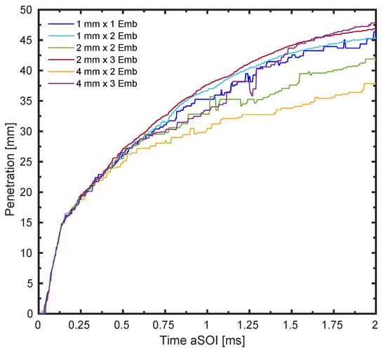
Figure 1.
Effect of different mesh base and minimum cell sizes on the spray penetration.
AMR is an effective tool in reducing the computational cost by refining the grid only in the region of interest. That being said, the refinement was performed based on the total fuel mass fraction, where the lower and upper thresholds were set to and 1, respectively. The field takes into account both liquid and vapor fuel fractions in a given cell and refines the cells according to the threshold limits. The calculations are performed in a rectangular domain of 110 width and 100 of height. The boundaries of the domain are all modeled as walls and the domain is large enough so that liquid parcels do not interact with them. The RANS approach was adopted for turbulence modeling. All simulations were carried out with the standard turbulence model with a turbulent dissipation constant, , of increased from a standard value of . The model was chosen due to the improved spray morphology and gas entrainment it entails as compared with other models, such as the RNG model [26]. Increasing the parameter is consistent with the “round jet correction” according to Pope and improves the spray jet morphology when the standard is used to resolve the turbulent field [27]. The turbulent kinetic energy and dissipation rate were initialized to 1 / and 90 /, respectively.
2.2. Spray Models
The approach utilizes the Discrete Droplet Method which signifies that suitable sub–models should be implemented to describe the introduction of parcels into the computational domain and the subsequent stages that the parcels undergo from primary atomization until liquid evaporation. The velocity profile of the Lagrangian parcels is directly proportional to the mass flow rate and inversely proportional to the area contraction coefficient , both of which are user inputs. The mass flow rate profile used was that of the well known ECN Spray G injector at 200 of injection pressure. The area contraction coefficient was set to 0.8 leading to an initial velocity of 150 / for the spray G1 baseline condition in this study. The Lagrangian field of the simulation was statistically represented by 60,000 parcels so as to have a suitable compromise between simulation run time and accuracy.
The primary breakup was modeled by the turbulence induced Huh Gosman atomization model [28]. The fuel is injected into constant volume chamber as spherical blobs with the same diameters as the orifice holes, 165 in this study. The model accounts for the turbulent motion at that nozzle outlet by producing an initial surface perturbation on the parcels. These perturbations grow due to the aerodynamic forces induced by the gas phase. The primary parcel diameter reduction rate is proportional to the ratio between the atomization length and time scales:
where is a tuning factor (value shown in Table 1). The characteristic atomization length scale is dependent on the turbulence length scale according to the relation:
where is the wavelength of surface perturbations induced by turbulence with (2.0) and (0.5). The atomization time scale is calculated from a linear combination of turbulent time and wave growth time scales:

Table 1.
Spray model constants.
The wave growth rate time scale is obtained from a formulation based on Kelvin–Helmholtz (KH) instability theory. Literature values for (1.2) and (0.5) were adopted. The turbulent length and time scales are evaluated using the turbulent kinetic energy k and its dissipation rate according to:
in Equations (4) and (5) is the same constant used in the turbulence model and equal to . The stripped mass, as a result of the diameter reduction in Equation (1), is calculated according to:
where is the liquid fuel density, is the particle number, the parent parcel diameter, and the newly computed diameter. The Huh Gosman model also predicts the initial plume cone angle according to the atomization length and time scales where the spray is assumed to diverge radially with a velocity proportional to the ratio between the atomization length and time scale. However, previous studies have shown that these correlations underpredict the spray cone angle for Spray G applications [29]. Therefore, the plume cone angle was imposed separately and the Huh Gosman model was only responsible for the primary atomization phase.
The break up of the secondary droplets stripped from parent parcels is goverened by the Kelvin–Helmholtz Rayleigh–Taylor (KHRT) breakup model. The distinction between the regions where primary atomization takes place and where the secondary break up activity takes control is defined by the so–called core length and is computed according to:
where is a parameter that takes into account flow conditions inside the injector, d is the injector orifice diameter, and and are the density of liquid and gas phase, respectively. Hence, the KH stripping activity is decoupled from the primary atomization process and is only applied after a certain distance from the injector tip. This was done in order to prevent excessive stripping due to the KH model in the near nozzle region that would lead to small droplet diameters which negatively influence the air entrainment and thus impacts the spray morphology. The KH stripping activity stems from the idea that each droplet has instabilities on its surface as it leaves the nozzle, similarly to what was mentioned previously in the Huh Gosman model. These instabilities grow due to the gas–liquid interaction resulting from high relative velocities. The wave growth rate is expressed by omega, , and its characteristic length by lambda, . The wave with the fastest growth rate will detach and create new droplets that will have a diameter proportional to and , where is a model constant usually set to . As a consequence, the parent parcel will lose some mass as child droplets are continuously detaching leading to a reduction of the parent droplet diameter according to:
with being the characteristic KH breakup time and expressed as:
can be tuned by operating on the model constant (value shown in Table 1). When the RT breakup model is triggered, the droplets undergo a catastrophic breakup event once they have passed a certain period of time that is equal to or greater than the characteristic time . Similarly to the model, the characteristic growth rate of the wave could be computed according to:
where is a model constant which accounts for the effects that create instabilities over the surface and requires careful calibration as it strongly effects the droplet diameter and velocity properties. is the surface tension and a is the acceleration that the droplet undergoes to the aerodynamic force that it is subjected to and is computed according to Equation (11):
which depends on the relative velocities between the liquid and gas, their densities, and the droplet drag coefficient . Once the condition for is satisfied, the disintegration of the parent droplet to a number of equally size droplets is done and the new diameter is set according to:
Liquid evaporation was modeled by a mass based approach [30] whenever flash boiling conditions were non–existent and the evaporation rate is expressed as:
in which D represents the droplet diameter, is the mass diffusion coefficient, is the Sherwood number, is the vapor fuel density, and and are the fuel vapor mass fractions evaluated at point in the far field and close to the droplet surface at saturation conditions, respectively. The term in parentheses is usually called the Spalding number and denoted by B. Equation (13) is only valid for evaporation without boiling. The reason is that if the evaporation pressure approaches the pressure of the system, B would tend to zero since the fuel vapor mass fraction at the droplet surface would tend to unity. This would lead to an unrealistic infinite evaporation rate which is not physical. Therefore, under flash boiling conditions, the Adachi Rutland flash boiling evaporation model [31,32] is implemented instead, where the heat exchange between the droplet interior and the surroundings control the phase change process rather than diffusion. The readers are advised to refer to the work of Paredi et al. [15] for a complete description of the model formulation and implementation in LibICE. The main constants for the spray sub–models are tabulated in Table 1.
2.3. Post–Processing Techniques
The post–processing fields and routines implemented throughout this paper are outlined in this section. Vapor penetration was numerically calculated based on the mixture fraction. It was defined by the distance from the nozzle tip position up to where % of mixture fraction was found. Axial liquid phase penetration were measured according to the projected liquid volume (PLV) fraction [33] which enables a direct comparison between experimental and CFD data. The procedure is based on the relation of the liquid volume fraction to the optical thickness of the liquid along the light path according to Equation (14):
where D is the droplet diameter taken as 7 according to Phase Doppler Interferometer (PDI) measurements provided by General Motors (GM) to the ECN and is the extinction cross–section acquired from MIE theory. It was assumed that the droplet diameter and extinction coefficient are constant along the light path. can be calculated using MiePlot [34] and is a function of the droplet diameter, light wavelength, and the collection angle of the optical setup. It was calculated to be for Spray G with iso–octane. The PLV indicates how much liquid volume is present in a certain projected area and thus has the units of (liquid)/ . Two different thresholds were used and recommended by ECN in order to reduce the uncertainties of the dependence on the chosen diameter value. Hence, a high and a low threshold were used according to Equations (15) and (16), respectively,
The PLV was numerically computed by integrating the Eulerian of the spray for different slices and projecting it on a two–dimensional plane. The liquid penetration was then deduced as the maximum axial position from the nozzle tip with a value below either of the thresholds. The axial gas velocity was computed by a probe point placed at 15 distance away from the injector tip location and was compared with Particle Image Velocimetry (PIV) measurements [35]. Finally, the radial Sauter Mean Diameter (SMD) distribution was computed along a line passing through one of the plumes at perpendicular plane 15 below the injector tip according to Figure 2 and was compared with experimental PDI measurements performed by GM [36].
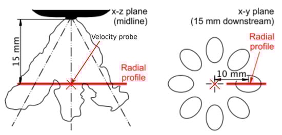
Figure 2.
Location of line probe for SMD data sampling and velocity measurement point [37].
2.4. Experimental Methodology
The experimental facility used to measure the flash boiling condition for all the fuels will be briefly discussed in this section. For a more detailed explanation about the optical techniques and post–processing algorithms, the readers are advised to refer to [38].
The injector used in the spray visualization measurements is the Spray G injector (serial AV67–026) used by the ECN [9]. It is a solenoid driven eight hole injector designed for Direct Injection Spark Ignition (DISI) engine configurations. The geometrical details of the injector are shown in Table 2.
Table 2.
Spray G injector characteristics.
The high pressure fuel system is similar to that used for diesel injectors and has been previously described in [39]. More importantly, the spray visualization was based on two optical techniques: single–pass schlieren was used for the vapor phase and diffused back illumination (DBI) for the liquid phase. The latter setup is shown in Figure 3, where the main optical components can be depicted. A blue light emitting diode (LED) light source was placed on one side of the test chamber where an engineered diffuser with 100 diameter was used leading to a uniform light transmission. A Fresnal lens characterized by a focal length of 67 was utilized in order to reproduce the diffused light at the optical plane of interest. The Photron S9 camera acquisition speed was set to 30 and the spatial resolution was / with a field of view of 384 × 376 pixels.
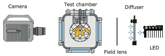
Figure 3.
DBI optical setup for liquid phase visualization.
The schlieren setup consisted of point illumination light source coming from a 1 Mercury–Xenon arc lamp. A parabolic mirror is used to parallelize the rays before passing through the test vessel. After passing through the chamber, the rays are converged at the focal length ( 450 ) of a biconvex lens where a diaphragm, with 4 cutoff diameter, is placed right before the high speed camera to provide a highly contrasted image, as shown in Figure 4. The high speed Photron SA5 camera acquisition rate was set to 30 and had a field of view of 512 × 512 pixels. The spatial resolution for the Schlieren technique was /. More details regarding the experimental facility and optical techniques utilized for this study could be found in [40]. The main methodology for image processing is detailed in Payri et al. [38].
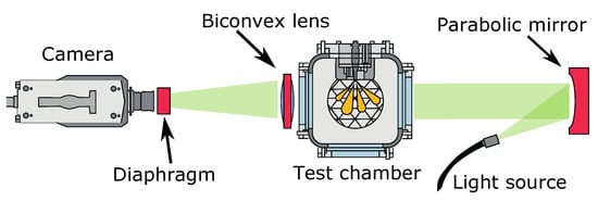
Figure 4.
Schlieren optical setup for liquid phase visualization.
2.5. Fuels and Test Conditions
The fuels used in the experimental campaign as well as in numerical simulations consist of gasoline fuel surrogates. Usually, iso–octane and n–heptane mixtures are used to simulate gasoline fuels with different octane numbers. For flash boiling conditions, fuel volatility becomes an important factor and for this reason various surrogate mono–component fuels are chosen with similar distillation curves of commercial gasoline. Table 3 displays the fuels used in this study along with the main properties. It is evident that the vapor pressure of fuels are quite different, leading to distinct behaviors under flash boiling conditions.
Table 3.
Properties of the fuels investigated obtained from NIST database [41].
Table 4 shows the operating conditions considered in this study. The baseline condition G1 was used to first validate the spray model with iso–octane. Following this stage, simulations were done for Spray G2 cold condition variant and compared with experimental measurements carried out at CMT–Motores Térmicos by the techniques described in Section 2.4 for the fuels previously shown. In addition, a total of 10 injection events, 160 frames each, were acquired for every G2 cold condition.
Table 4.
Operating conditions.
3. Results and Discussion
3.1. Baseline G1 Condition
The numerical spray model was first validated for the Spray G baseline condition (G1). The most important spray macroscopic parameters are compared with Sandia’s experimental measurements for vapor and liquid penetration. In addition, the spray–air interaction and gas entrainment were assessed based on centerline axial gas velocity from PIV measurements and finally, the performance of the stripping and break up activity of the KHRT model was verified based on SMD measurements provided by GM at different time steps.
The results shown in this section are an outcome of an extensive calibration procedure carried out in order to establish a suitable baseline model able to predict the aforementioned variables and to be extended to flash boiling conditions for the various fuels evaluated in this study. Therefore, it must be said that the constants implemented in the models are not intended to be the ideal ones for one operating condition but rather provide a comprehensive setup in order to predict the spray evolution for all the conditions investigated.
The evolution of the axial vapor phase penetration is shown in Figure 5. Initially, the model slightly overpredicts the vapor speed and penetrates with a steeper slope for the first milliseconds. The curve then seems to follow the experimental profile reasonably well and is capable of capturing the shape of the experimental curve. After the end of injection, the momentum of the spray seems to be lower than the experimental one where a slight deviation initiates and the numerical vapor penetrates with a slightly lower rate. Overall, it could be stated that the adopted turbulence model and Pope correction for the constant predict the air–fuel mixing process quite well and thus the spray evaporation rate. The issue with the underprediction after the end of injection (EOI) could be related to the adopted numerical cell resolution, in other words, refining the domain with an additional level of refinement could enhance the results considering a fixed spray model setup. However, a minimum value of was considered sufficient enough to provide a good compromise between simulation run time and accuracy.
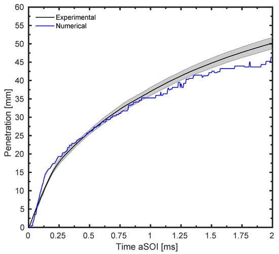
Figure 5.
Numerical and experimental axial vapor phase penetration for the baseline condition (G1).
Liquid phase axial penetration results are displayed in Figure 6 where both thresholds are shown. Comparing results with two different thresholds provides detailed feedback on whether the deviations from experimental data is related to the tip of the spray plume or to the region nearby the liquid core. The low threshold captures most of the liquid length up to the spray plume tip whereas the high threshold only captures the dense liquid region. Observing the initial stage of injection, it could be seen that the axial liquid penetration for both thresholds is higher than the experimental curves. That is mainly attributed to the prolonged core length which allows larger droplets to evolve for a longer distance since the KH stripping activity is not active within this region. That being said, a shorter liquid core length could be implemented by decreasing the constant in order to trigger the KH stripping activity sooner. However, considering the current setup, it was concluded by the authors that for the given stripping characteristics, very small droplets will be present in the near nozzle region which would negatively influence the gas entrainment and spray morphology and increase the error in droplet size prediction; therefore, the selected value is justified. Following the early stage of injection, the low threshold liquid penetration follows the experimental trace quite effectively for the remainder of the injection duration as well as EOI. On the other hand, the high threshold trend develops with a lower penetration magnitude compared to the experimental trace. The liquid residence time matches that of experimental data where it can be seen that the penetration value goes to zero at approximately . A sensitivity analysis done by the authors revealed that the reason for this underestimation of the high threshold is mainly due to two factors, the stripping intensity of the KH model, and the breakup of the RT model regulated by the constant. Hence, further tuning of the spray breakup model could enhance the trend of the high threshold liquid penetration curve, although the effect on the G2 cold condition should be carefully considered. It is of utmost importance to keep in mind the significance of these constants and their impact on the droplet diameters and consequently on the liquid evaporation rate when a calibration procedure is to be done.
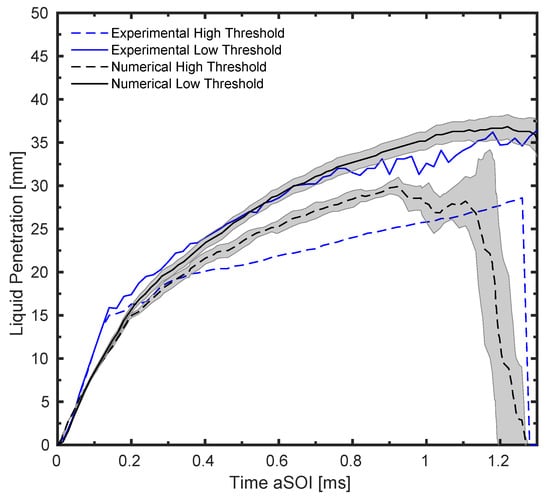
Figure 6.
Numerical and experimental axial liquid phase penetration for the baseline condition (G1). High threshold corresponds to / while low threshold corresponds to / liquid volume fraction.
In order to accurately predict the mixture formation process, the spray induced gas velocity is of vital importance as it directly influences the spray evaporation rate. For this reason, the centerline axial gas velocity at 15 downstream of the injector is calculated and is shown in Figure 7. The magnitude of the axial velocity is highly dependent on the turbulence model adopted and the liquid core length, or in other words, the location at which the transition from primary atomization regime to secondary breakup occurs. The computed axial gas velocity presents an overestimation of the recirculating gas motion during the injection phase. This can be attributed to the prolonged liquid core length resulting in bigger droplets for a larger distance leading to a higher gas entrainment. Consequently, the reverse motion of the gas phase is delayed as seen by the gap after the end of injection, at , and then follows the experimental trend with good accuracy.
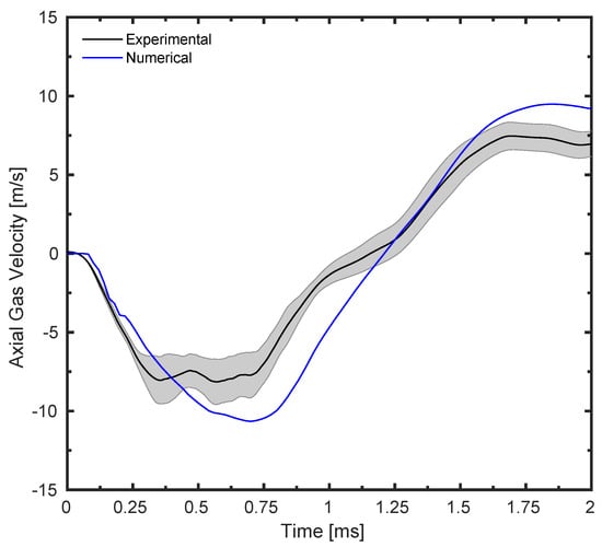
Figure 7.
Numerical axial gas velocity comparison with PIV experimental data from Sandia for the baseline condition (G1).
The assessment of the doplet SMD allowed for the evaluation of the performance of the breakup and stripping phases that the liquid droplets undergo as they are injected into the ambient gas. Figure 8 depicts the SMD values at three different time steps. An intense KH stripping activity at 0.3 ms leads to small droplets compared with experimental PDI measurements whereas a better agreement is reached during the late stage of injection and after EOI.
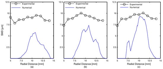
Figure 8.
Numerical radial SMD profile comparison with experimental PDI data from GM for the baseline condition (G1). (a) , (b) and (c) .
Spray morphology and liquid evaporation were also investigated based on the projected liquid volume maps. This permits a one–to–one comparison between computed and experimental liquid profiles and allows one to further elaborate the liquid penetration trends. The PLV data used in this comparison was obtained from the University of Melbourne (UoM) [15]. From Figure 9, it can be clearly seen that the numerical spray has a smaller plume cone angle with respect to the measurements. In addition, the computed spray seems to be denser with a higher liquid concentration on the plume tips. At , there is almost no liquid present in the domain which is not the case for the computed spray signifying a lower evaporation rate. Future efforts will investigate plume angles greater than the adopted value (16°) in order to be in agreement with the experimental morphology. Furthermore, the evaporation rate could also be simultaneously improved since the spray would entrain more air with a wider plume angle. It can also be noted that the numerical spray evolves with a larger spray width which could be attributed to the adopted drill angle in this study, 37. There are various uncertainties in literature [15,42] regarding the optimal drill angle value. Therefore, the drill angle was not used as a tuning factor in this study and the value of 37 was kept constant for all the simulations. Overall, the computed macroscopic and microscopic variables were deemed accurate and suitable to proceed with the study.
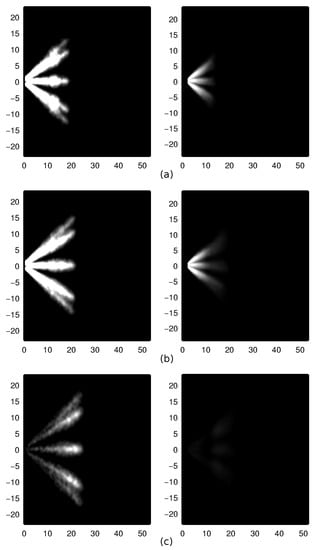
Figure 9.
Numerical (left) vs. UoM experimental (right) PLV maps for the baseline condition (G1). (a) at , (b) at and (c) at after SOI. Liquid volume fraction range is 0– /.
3.2. G2 Cold Condition for iso–octane
Following a thorough validation of the baseline G1 condition, the spray model was then used to simulate the G2 cold condition. Iso–octane was first analyzed since it was the liquid fuel with which the model was developed and calibrated. The only parameter that was changed from the previous model setup was the spray cone angle and was increased to to account for the mild flash boiling condition [43]. In the following analysis, for iso–octane and the different fuels that will be presented, the experimental data correspond to those described in Section 2.4 which were carried out at CMT. The numerical axial vapor and liquid penetrations are compared with the experimental ones and shown in Figure 10. The computed vapor penetration develops with a higher penetration magnitude for the majority of the injection duration as well as EOI. The trend, however, is captured by the numerical model. On the other hand, liquid penetration results agree with the experimental measurements although they present an overestimation during the steady phase of the injection duration due to the extended liquid core length. The slope of the curve is also predicted by the model well after the EOI. The results of vapor and liquid penetration indicate that there is more improvement to be done in terms of spray atomization and breakup in this weakly evaporative condition. The promotion of a more intense KH stripping activity, leading to a higher evaporation rate, would provide enhanced behavior in terms of the vapor penetration results. Overall, the results shown are quite promising given that the model is able to predict the main macroscopic variables under different ambient densities and temperatures.
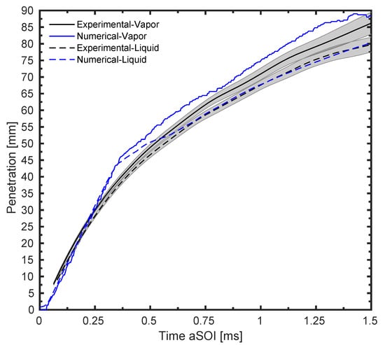
Figure 10.
Numerical and experimental axial vapor and liquid phases penetration for the G2 cold condition for iso–octane.
Furthermore, the spray morphologies are analyzed in terms of DBI images and images of the numerical spray parcels. The previous comparison demonstrated in Section 3.1 based on the projected liquid volume fraction could not be done here since the experimental measurements were not post–processed in this manner. Nevertheless, this method of comparison outlines the overall spray shape and permits the assessment of the spray behavior under mild flashing conditions. Figure 11 reports the evolution of the liquid during the injection event, at and , as well as after the end of injection at . The numerical model seems to capture the global spray shape and exhibits a certain degree of plume–to–plume interaction from the early stages of injection. In addition, the spray tip liquid density is also well captured although numerical images indicate that the overall plume width is wider than the corresponding DBI images. The liquid distribution is also predicted by the numerical model, especially at where few droplets appear in the liquid core region which agrees with the DBI images. It could then be stated that evaporation model utilized for the G2 cold condition is capable of reproducing the overall spray shape with good accuracy. That being said, the model is further analyzed in the next sections for several fuels which present different behaviors under mild flash boiling conditions.
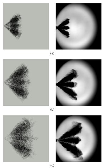
Figure 11.
Numerical (left) vs. CMT experimental (right) liquid morphology images for the G2 cold condition for iso–octane. (a) at , (b) at and (c) at after SOI.
3.3. G2 Cold Condition for n–heptane
This section is dedicated to the implementation of the numerical spray model with n–heptane. Given that n–heptane possesses similar liquid properties as iso–octane, the behavior under mild flashing conditions is expected to be similar as well. As what was previously discussed, the axial vapor and liquid phase penetrations are first examined and the spray morphologies through numerical and DBI images are then studied. Figure 12 shows the evolution of the vapor and liquid phases. The vapor phase follows the experimental trend quite well up to the end of injection. A slight underestimation can then be observed in the range of to ; however, the deviation from the experimental trace is considered negligible. The same could be said for the axial liquid penetration, where the slight overestimation during the initial stages of injection is present, as previously seen with iso–octane.
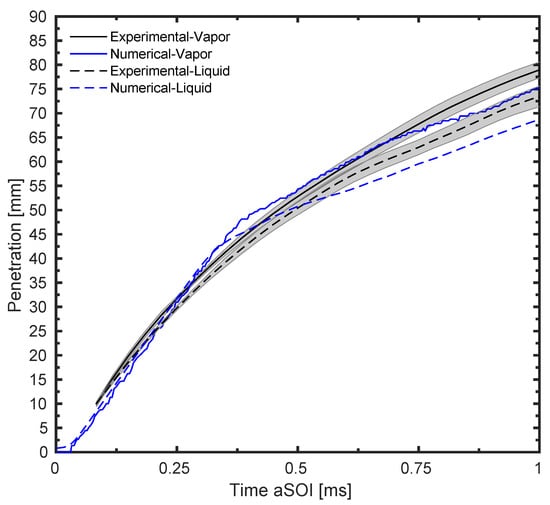
Figure 12.
Numerical and experimental axial vapor phases penetration for the G2 cold condition for n–heptane.
The evolution of the spray morphology during and after the end of injection is shown in Figure 13. Experimental and numerical images resemble that of iso–octane where plume–to–plume interaction is evident. The effect of superheated liquid on the plume radial expansion as well as the Adachi Rutland flash boiling diameter reduction rate seem to accurately predict the flashing behavior using n–heptane as a fuel. So far, the fuel tested are said to be in mild flashing conditions since the values are slightly greater than unity. The value is generally used to indicate the presence of flash boiling and is computed according to the ratio of fuel saturation to ambient pressure /. The value for n–heptane under the G2 cold condition is around . The next sections will feature the remaining fuels investigated in this study, n–hexane and n–pentane, which are characterized by a higher superheat degree compared to iso–octane and n–heptane.
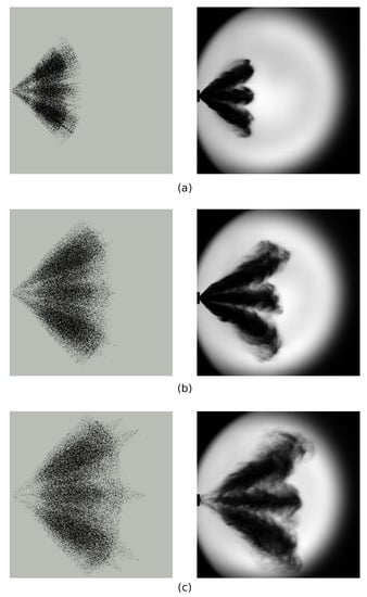
Figure 13.
Numerical (left) vs. CMT experimental (right) liquid morphology images for the G2 cold condition for n–heptane. (a) at , (b) at and (c) at after SOI.
3.4. G2 Cold Condition for n–hexane
N–hexane is usually employed to imitate the light component of gasoline and previous experimental studies under flash boiling conditions have shown that its behavior is more similar to gasoline compared to n–heptane and iso-octane [44]. Validation for the axial vapor and liquid phase penetrations is shown in Figure 14. The computed profiles correctly match the experimental trends for the whole injection duration and the model is able to reproduce the higher volatility characteristic of n–hexane compared to the previous fuels, as can be seen by the reduced penetration length. The Adachi Rutland implemented model thus proves to be accurate in computing the evaporation rate in weakly evaporative conditions and for fuels of different volatilities.
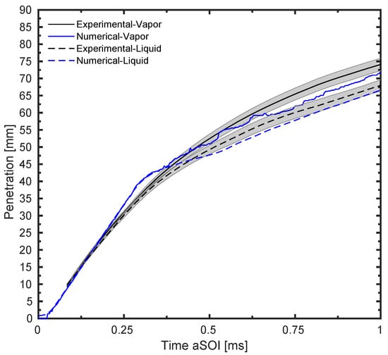
Figure 14.
Numerical and experimental axial vapor and liquid phases penetration for the G2 cold condition for n–hexane.
To further assess the numerical results, the spray morphology is depicted in Figure 15. A clear difference can be seen in the DBI images compared to the fuels previously elaborated. Thicker plumes are now evident leading to a strong plume–to–plume interference although distinct spray plumes can still be observed. Therefore, the radial expansion of the plumes due to flash boiling is more evident for n–hexane. The numerical images further confirm the reduced liquid penetration of n–heptane. Moreover, the spray tip shape is also captured by the computed spray in the stable phase of injection at . This could also be extended to shortly after the injection has ended.
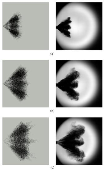
Figure 15.
Numerical (left) vs. CMT experimental (right) liquid morphology images for the G2 cold condition for n–hexane. (a) at , (b) at , and (c) at after SOI.
3.5. G2 Cold Condition for n–pentane
N–pentane encompasses the highest value among all the fuels tested; therefore, a more extreme case of flash boiling is expected. After a thorough calibration procedure, the authors concluded that a slightly smaller plume cone angle, 23, compared to the previous fuels should be adopted to accurately describe the spray development into the gas phase. Figure 16 shows the axial vapor and liquid penetrations. It can be clearly seen that the computed liquid phase evolution has a different slope than the experimental one which is magnified after the end of injection and a large deviation is present. This implies that the acceleration of penetration due to the spray collapse is not captured by the model.
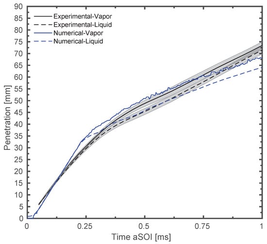
Figure 16.
Numerical and experimental axial vapor and liquid phases penetration for the G2 cold condition for n–pentane.
A more detailed explanation of the deviation shown in Figure 16 could be drawn from the spray morphology images shown in Figure 17. A large discrepancy between the numerical and experimental images can be clearly seen. At , the experimental spray is already collapsed towards the injector axis and evolves as a single entity. In addition, an initiation of the toroidal structure is seen at the spray radial extremities. This behavior is not reproduced by the numerical model where the plumes continue to penetrate in their original direction with minor plume–to–plume interactions. At , the toroidal structure becomes more evident and a higher degree of recirculating motion is shown at the two radial extremities of the spray. The tip of the numerical spray slightly changes and becomes narrower. Finally, after the end of injection at , the experimental spray penetrates faster due to the spray collapse. No spray collapse is evident in the numerical spray although a slight deviation of parcel direction at the spray tip can be noticed. The variation in the slopes of the liquid penetration curves between the numerical and experimental trends can then be justified by the spray images. The numerical model presents a drawback since the spray collapse is not predicted and therefore lags behind in terms of penetration. Duronio et al. [45] adjusted the plume direction and cone angle when moving towards more extreme case of flash boiling at an ambient density of / and using iso–octane. The plume direction was decreased down to 19, compared to the nominal 37, and it was possible to reproduce the spray collapse by doing so. Modifying the plume cone angle and plume direction produced a higher radial velocity component in the spray simulations leading to the classical bell shape of the jet with two recirculation zones on each side. However, for the sake of implementing a comprehensive model, the plume direction was not modified in this study and the plume cone angle reduction alone was not able to predict the spray collapse behavior seen in the experimental images.
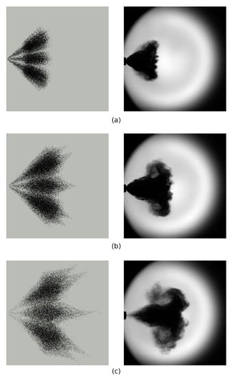
Figure 17.
Numerical (left) vs. CMT experimental (right) liquid morphology images for the G2 cold condition for n–pentane. (a) at , (b) at and (c) at after SOI.
4. Conclusions and Outlook
The current study comprised of the implementation of Lagrangian spray simulations for a multi–hole gasoline direct injector, Spray G from the ECN, and several mono–component fuels with different physical characteristics. The eight–hole injector was tested, both numerically and experimentally, under the baseline G1 condition typical of a late injection strategy in a GDI engine and under the mild flash boiling condition (G2 cold) typical of part load operation. The experimental analysis was carried out in a constant volume chamber constructed for GDI spray visualizations at CMT–Motores Térmicos, whereas the computational part was developed within the OpenFOAM framework coupled with the LibICE code, developed by the ICE group of Politecnico di Milano for specific CFD applications applied to internal combustion engines.
Due to the abundance of experimental data for the Spray G1 condition, preliminary work involved tuning the spray sub–models for that case, reproducing the main variables made available by the ECN. The model was then left unchanged for the subsequent stages of the study where only the spray cone angle was varied to account for flash boiling evaporation. To this end, the validation process of the spray model did not only cover the vapor and liquid penetration comparison but rather included the assessment of the spray gas interaction by analyzing the axial gas centerline velocity, SMD radial distributions, and finally liquid spray morphologies. The RANS standard turbulence model with the Pope correction provided accurate results for the vapor phase penetration and the centerline axial gas velocity. A slight underestimation of the vapor penetration between and could be improved by further refining the grid; however, an increase in computational cost is expected. Likewise, adopting a fixed grid instead of using AMR could lead to a better prediction of the gas velocity since the centerline point bounded by the spray plumes would not be refined when AMR is utilized. Furthermore, liquid high and low threshold penetrations revealed that the liquid core of the spray is overpredicted which was verified by the morphology images although a better assessment would be done if PLV images from Sandia were available. Additionally, computed SMD values were quite a bit lower than the measured ones indicating that further tuning of the sub–models is required in order to accurately predict the diameters while maintaining an adequate liquid evaporation rate. Nonetheless, the adopted setup was evaluated to be suitable for the investigation of the flash boiling behavior of the various fuels.
Iso–octane and n–heptane both demonstrated similar behaviors under mild flashing conditions. The radial expansion of the spray was slightly overestimated as shown by the comparison of the numerical parcel and experimental DBI images. A more comparative assessment would be to compare the morphologies in the same way done for the Spray G1 condition since the same post–processing and thresholding procedure would be employed for both images. In any case, the plume–to–plume interaction was captured by the numerical model for both fuels. The Adachi–Rutland evaporation rate and flashing diameter reduction led to a good agreement between numerical and experimental penetration trends. Therefore, the adopted spray setup tuned for the G1 condition was also able to predict the main spray characteristics even at three times lower ambient density without the need of a re–calibration. The adopted methodology was also validated under a more intense flash boiling scenario by testing n–hexane under the same chamber conditions. The computed liquid and vapor penetrations were in good agreement with the measured profiles for the whole duration of injection. Spray morphology images indicated that the numerical model is weak in capturing the radial expansion of the dense liquid core region due to the intense flash boiling phenomenon although a good agreement is observed at the plume tips. The weakness of the DDM model is further magnified when n–pentane was investigated. The underestimation of the liquid phase penetration and liquid spray morphologies demonstrated that the numerical spray model did not contract and thus evolved with an overall lower penetration. This highlights an important limitation in the adopted methodology and lays the foundation for future development activities that must be carried out. In that sense, it must be said that the physics occurring inside the nozzle and near nozzle region cannot be neglected under extreme cases of flash boiling leading to spray collapse. Therefore, future activities are intended to implement a coupling between internal and external nozzle flow so that the initial plume direction and cone angle are calculated by the internal nozzle flow Eulerian model which initializes the Lagrangian simulation. This would be a more physical approach rather than imposing fixed injection direction and plume angle values, making the model less reliant on experimental measurements. In addition, the rapid phase change and plume expansion occurring at the nozzle exit under flash boiling conditions could be captured and transmitted to the subsequent Lagrangian simulation, thus improving the model fidelity.
Author Contributions
Conceptualization, R.P., R.A. and A.B.; methodology, P.M.-A., R.A. and A.B.; software, R.A. and A.B.; validation, P.M.-A. and R.A.; formal analysis, R.A.; investigation, R.P. and A.B.; resources, R.P.; data curation, R.P.; writing—original draft preparation, R.A.; writing—review and editing, R.P. and P.M.-A.; visualization, P.M.-A., R.A. and A.B.; supervision, R.P. and P.M.-A.; project administration, R.P.; funding acquisition, R.P. All authors have read and agreed to the published version of the manuscript.
Funding
This research was funded by Ministerio de Ciencia, Innovación y Universidades grant number RTI2018–099706–B–I00 in the frame of the project Study of Primary Early Atomization using DNS and Optical Ultra–high resolution Techniques (SPREAD OUT). Additionally, the PhD student Rami Abboud has been funded by Ayudas para la formación de profesorado universitario (FPU) program with reference FPU19/03838.
Institutional Review Board Statement
Not applicable.
Informed Consent Statement
Not applicable.
Conflicts of Interest
The authors declare no conflict of interest.
References
- Millo, F.; Gullino, F.; Rolando, L. Methodological approach for 1D simulation of port water injection for knock mitigation in a turbocharged DISI engine. Energies 2020, 13, 4297. [Google Scholar] [CrossRef]
- Tornatore, C.; Sjöberg, M. Optical investigation of a partial fuel stratification strategy to stabilize overall lean operation of a DISI engine fueled with gasoline and E30. Energies 2021, 14, 396. [Google Scholar] [CrossRef]
- Gong, C.; Si, X.; Liu, F. Combined effects of excess air ratio and EGR rate on combustion and emissions behaviors of a GDI engine with CO2 as simulated EGR (CO2) at low load. Fuel 2021, 293, 120442. [Google Scholar] [CrossRef]
- Huang, W.; Gong, H.; Moon, S.; Wang, J.; Murayama, K.; Taniguchi, H.; Arima, T.; Arioka, A.; Sasaki, Y. Nozzle Tip Wetting in GDI Injector at Flash-boiling Conditions. Int. J. Heat Mass Transf. 2021, 169, 120935. [Google Scholar] [CrossRef]
- Fach, C.; Rödel, N.; Schorr, J.; Krüger, C.; Dreizler, A.; Böhm, B. Multi-parameter imaging of in-cylinder processes during transient engine operation for the investigation of soot formation. Int. J. Engine Res. 2021. [Google Scholar] [CrossRef]
- Kale, R.; Banerjee, R. Optical investigation of flash boiling and its effect on in-cylinder combustion for butanol isomers and iso-octane. Int. J. Engine Res. 2021, 22, 1565–1578. [Google Scholar] [CrossRef]
- Du, J.; Mohan, B.; Sim, J.; Fang, T.; Roberts, W.L. Study of spray structure under flash boiling conditions using 2phase-SLIPI. Exp. Fluids 2021, 62, 24. [Google Scholar] [CrossRef]
- Chang, M.; Lee, Z.; Park, S.; Park, S. Characteristics of flash boiling and its effects on spray behavior in gasoline direct injection injectors: A review. Fuel 2020, 271, 117600. [Google Scholar] [CrossRef]
- Engine Combustion Network. Available online: https://ecn.sandia.gov/gasoline-spray-combustion/ (accessed on 30 September 2020).
- Mohapatra, C.K.; Schmidt, D.P.; Sforozo, B.A.; Matusik, K.E.; Yue, Z.; Powell, C.F.; Som, S.; Mohan, B.; Im, H.G.; Badra, J.; et al. Collaborative investigation of the internal flow and near-nozzle flow of an eight-hole gasoline injector (Engine Combustion Network Spray G). Int. J. Engine Res. 2020. [Google Scholar] [CrossRef]
- Shahangian, N.; Sharifian, L.; Miyagawa, J.; Bergamini, S.; Uehara, K.; Noguchi, Y.; Marti-aldaravi, P.; Martinez, M.; Payri, R. Nozzle Flow and Spray Development One-Way Coupling Methodology for a Multi-Hole GDi Injector. SAE Tech. Pap. Ser. 2019. [Google Scholar] [CrossRef]
- Kong, S.C.; Senecal, P.K.; Reitz, R.D. Developments in spray modeling in diesel and direct-injection gasoline engines. Oil Gas Sci. Technol. 1999, 54, 197–204. [Google Scholar] [CrossRef]
- Duronio, F.; Ranieri, S.; Montanaro, A.; Allocca, L.; De Vita, A. ECN Spray G injector: Numerical modelling of flash-boiling breakup and spray collapse. Int. J. Multiph. Flow 2021, 2021, 103817. [Google Scholar] [CrossRef]
- Wadekar, S.; Yamaguchi, A.; Oevermann, M. Large-Eddy Simulation Study of Ultra-High Fuel Injection Pressure on Gasoline Sprays. Flow Turbul. Combust. 2021, 107, 149–174. [Google Scholar] [CrossRef]
- Paredi, D.; Lucchini, T.; D’Errico, G.; Onorati, A.; Pickett, L.; Lacey, J. Validation of a comprehensive computational fluid dynamics methodology to predict the direct injection process of gasoline sprays using Spray G experimental data. Int. J. Engine Res. 2020, 21, 199–216. [Google Scholar] [CrossRef]
- Jiang, C.; Parker, M.C.; Helie, J.; Spencer, A.; Garner, C.P.; Wigley, G. Impact of gasoline direct injection fuel injector hole geometry on spray characteristics under flash boiling and ambient conditions. Fuel 2019, 241, 71–82. [Google Scholar] [CrossRef] [Green Version]
- Sun, Z.; Cui, M.; Ye, C.; Yang, S.; Li, X.; Hung, D.; Xu, M. Split injection flash boiling spray for high efficiency and low emissions in a GDI engine under lean combustion condition. Proc. Combust. Inst. 2021, 38, 5769–5779. [Google Scholar] [CrossRef]
- Sun, Z.; Yang, S.; Nour, M.; Li, X.; Hung, D.; Xu, M. Significant Impact of Flash Boiling Spray on In-Cylinder Soot Formation and Oxidation Process. Energy Fuels 2020, 34, 10030–10038. [Google Scholar] [CrossRef]
- Dong, X.; Yang, J.; Hung, D.L.; Li, X.; Xu, M. Effects of flash boiling injection on in-cylinder spray, mixing and combustion of a spark-ignition direct-injection engine. Proc. Combust. Inst. 2019, 37, 4921–4928. [Google Scholar] [CrossRef]
- Lacey, J.; Poursadegh, F.; Brear, M.J.; Gordon, R.; Petersen, P.; Lakey, C.; Butcher, B.; Ryan, S. Generalizing the behavior of flash-boiling, plume interaction and spray collapse for multi-hole, direct injection. Fuel 2017, 200, 345–356. [Google Scholar] [CrossRef]
- Li, Y.; Guo, H.; Zhou, Z.; Zhang, Z.; Ma, X.; Chen, L. Spray morphology transformation of propane, n-hexane and iso-octane under flash-boiling conditions. Fuel 2019, 236, 677–685. [Google Scholar] [CrossRef]
- Nocivelli, L.; Sforzo, B.A.; Tekawade, A.; Yan, J.; Powell, C.F.; Chang, W.; Lee, C.F.; Som, S. Analysis of the Spray Numerical Injection Modeling for Gasoline Applications; SAE Technical Papers; SAE International: Warrendale, PA, USA, 2020. [Google Scholar] [CrossRef]
- Weller, H.G.; Tabor, G.; Jasak, H.; Fureby, C. A tensorial approach to computational continuum mechanics using object-oriented techniques. Comput. Phys. 1998, 12, 620–631. [Google Scholar] [CrossRef]
- Lucchini, T.; D ’errico, G.; Ettorre, D. Numerical investigation of the spray-mesh-turbulence interactions for high-pressure, evaporating sprays at engine conditions. Int. J. Heat Fluid Flow 2011. [Google Scholar] [CrossRef]
- Lucchini, T.; D’Errico, G.; Paredi, D.; Sforza, L.; Onorati, A. CFD Modeling of Gas Exchange, Fuel-Air Mixing and Combustion in Gasoline Direct-Injection Engines; SAE Technical Papers; SAE International: Warrendale, PA, USA, 2019. [Google Scholar] [CrossRef]
- Paredi, D. CFD Modeling and Validation of Spray Evolution in Gasoline Direct Injection Engines. Ph.D. Thesis, Politecnico di Milano, Milan, Italy, 2020. [Google Scholar]
- Pope, S.B. An explanation of the turbulent round-jet/plane-jet anomaly. AIAA J. 1978, 16, 279–281. [Google Scholar] [CrossRef]
- Huh, K.Y.; Gosman, A.D. A Phenomenological Model of Diesel Spray Atomization. In Proceedings of the International Conference on Multiphase Flows, Tsukuba, Japan, 24–27 September 1991. [Google Scholar]
- Paredi, D.; Lucchini, T.; D’Errico, G.; Onorati, A.; Montanaro, A.; Allocca, L.; Ianniello, R. Combined Experimental and Numerical Investigation of the ECN Spray G under Different Engine-Like Conditions; SAE Technical Papers; SAE International: Warrendale, PA, USA, 2018. [Google Scholar] [CrossRef] [Green Version]
- Baumgarten, C. Mixture Formation in IC Engines; Springer: Berlin/Heidelberg, Germany, 2006. [Google Scholar]
- Adachi, M.; McDonell, V.G.; Tanaka, D.; Senda, J.; Fujimoto, H. Characterization of Fuel Vapor Concentration inside a Flash Boiling Spray; SAE Technical Papers; SAE International: Warrendale, PA, USA, 1997. [Google Scholar] [CrossRef]
- Zuo, B.; Gomes, A.M.; Rutland, C.J. Modelling superheated fuel sprays and vaproization. Int. J. Engine Res. 2000, 1, 321–336. [Google Scholar] [CrossRef]
- Engine Combustion Network. Available online: https://ecn.sandia.gov/ecn-workshop/ecn6-workshop/ (accessed on 17 November 2020).
- A Computer Program for Scattering of Light from a Sphere Using Mie Theory & the Debye Series. Available online: http://www.philiplaven.com/mieplot.htm (accessed on 3 March 2021).
- Sphicas, P.; Pickett, L.M.; Skeen, S.; Frank, J.; Lucchini, T.; Sinoir, D.; D’Errico, G.; Saha, K.; Som, S. A Comparison of Experimental and Modeled Velocity in Gasoline Direct-Injection Sprays with Plume Interaction and Collapse. SAE Int. J. Fuels Lubr. 2017, 10, 184–201. [Google Scholar] [CrossRef]
- ECN, Engine Combustion Network—Primary Spray G Datasets. Available online: https://ecn.sandia.gov/gasoline-spray-combustion/target-condition/primary-spray-g-datasets/ (accessed on 25 January 2021).
- Duke, D.J.; Kastengren, A.L.; Matusik, K.E.; Swantek, A.B.; Powell, C.F.; Payri, R.; Vaquerizo, D.; Itani, L.; Bruneaux, G.; Grover, R.O.; et al. Internal and near nozzle measurements of Engine Combustion Network “Spray G” gasoline direct injectors. Exp. Therm. Fluid Sci. 2017, 88, 608–621. [Google Scholar] [CrossRef] [Green Version]
- Payri, R.; Salvador, F.J.; Abboud, R.; Viera, A. Study of evaporative diesel spray interaction in multiple injections using optical diagnostics. Appl. Therm. Eng. 2020, 176, 115402. [Google Scholar] [CrossRef]
- Payri, R.; Bracho, G.; Gimeno, J.; Bautista, A. Rate of injection modelling for gasoline direct injectors. Energy Convers. Manag. 2018, 166, 424–432. [Google Scholar] [CrossRef]
- Rodriguez, A.B. Study of the Gasoline Direct Injection Process under Novel Operating Conditions. Ph.D. Thesis, Universitat Politècnica de València, Valencia, Spain, 2021. [Google Scholar]
- Lemmon, E.W.; McLinden, M.O.; Friend, D.G. Thermophysical Properties of Fluid Systems. In NIST Chemistry WebBook, NIST Standard Reference Database Number 69; Linstrom, P.J., Mallard, W.G., Eds.; National Institute of Standards and Technology: Gaithersburg, MD, USA, 2011; p. 20899. [Google Scholar] [CrossRef]
- Payri, R.; Gimeno, J.; Marti-Aldaravi, P.; Martínez, M. Nozzle Flow Simulation of Gdi for Measuring Near-Field Spray Angle and Plume Direction; SAE Technical Papers; SAE International: Warrendale, PA, USA, 2019; pp. 1–11. [Google Scholar] [CrossRef]
- Guo, H.; Li, Y.; Lu, X.; Zhou, Z.; Xu, H.; Wang, Z. Radial expansion of flash boiling jet and its relationship with spray collapse in gasoline direct injection engine. Appl. Therm. Eng. 2019, 146, 515–525. [Google Scholar] [CrossRef]
- Araneo, L.; Donde’, R. Flash boiling in a multihole G-DI injector—Effects of the fuel distillation curve. Fuel 2017, 191, 500–510. [Google Scholar] [CrossRef]
- Duronio, F.; De Vita, A.; Allocca, L.; Montanaro, A.; Ranieri, S.; Villante, C. CFD Numerical Reconstruction of the Flash Boiling Gasoline Spray Morphology; SAE Technical Papers; SAE International: Warrendale, PA, USA, 2020. [Google Scholar] [CrossRef]
Publisher’s Note: MDPI stays neutral with regard to jurisdictional claims in published maps and institutional affiliations. |
© 2021 by the authors. Licensee MDPI, Basel, Switzerland. This article is an open access article distributed under the terms and conditions of the Creative Commons Attribution (CC BY) license (https://creativecommons.org/licenses/by/4.0/).