Research Progress of Oilfield Development Index Prediction Based on Artificial Neural Networks

Abstract

Accurately predicting oilfield development indicators (such as oil production, liquid production, current formation pressure, water cut, oil production rate, recovery rate, cost, profit, etc.) is to realize the rational and scientific development of oilfields, which is an important basis to ensure the stable production of the oilfield. Due to existing oilfield development index prediction methods being difficult to accurately reflect the complex nonlinear problem in the oil field development process, using the artificial neural network, which can predict the oilfield development index with the function of infinitely close to any non-linear function, will be the most ideal prediction method at present. This article summarizes four commonly used artificial neural networks: the BP neural network, the radial basis neural network, the generalized regression neural network, and the wavelet neural network, and mainly introduces their network structure, function types, calculation process and prediction results. Four kinds of artificial neural networks are optimized through various intelligent algorithms, and the principle and essence of optimization are analyzed. Furthermore, the advantages and disadvantages of the four artificial neural networks are summarized and compared. Finally, based on the application of artificial neural networks in other fields and on existing problems, a future development direction is proposed which can serve as a reference and guide for the research on accurate prediction of oilfield development indicators.

1. Introduction

The change characteristics of oilfield development indicators are regarded as an important basis for decision-making management issues such as oilfield development planning, oilfield development status evaluation, oilfield development plan design and adjustment, oilfield development risk prediction, and early warning [1]. Therefore, it is possible to reasonably grasp the future trend of oilfield development by mining oilfield development data and accurately predicting oilfield development indicators, and it is an important basis for achieving the stable development of crude oil production and formulating reasonable countermeasures to slow production. This is because there are many factors affecting oilfield development indicators, and these factors are mutually coupled, resulting in the attracted widespread attention from the majority of scientific researchers [2].

Oilfield development is a very complex process, and its production environment and production status are difficult to grasp. Therefore, accurate and efficient prediction of oilfield development indicators can help oilfield enterprise decision-makers fully grasp the current situation and future change trends of oilfield development and provide scientific, theoretical, and technical support for efficient and sustainable oilfield development. At present, the commonly used methods for predicting development indicators of oilfields mainly include numerical simulation, physical experiment, and multi-dimensional regression analysis [3]. Due to the complex non-linear relationship between oilfield development indicators and their influencing factors [4], the existing oilfield development indicator prediction methods have large errors. Artificial neural networks have strong self-learning and self-adaptive ability, and its strong nonlinear approximation ability enables it to approach the actual value of the measured object well [5]. Using artificial neural networks and intelligent algorithms to optimize neural networks and to predict the oilfield development indicators [6,7,8] is currently the most ideal prediction method.

This article summarizes several ANNs that can be used to predict oilfield development indicators, and conducts detailed analysis and comparison from the aspects of network structure, calculation process, optimization algorithm, advantages and disadvantages, etc., and has a certain guiding role in the research of future oilfield development indicator prediction models.

In order to evaluate the effectiveness of the included research results, WoS was used to search all articles of artificial neural networks in the oil and gas industry from 2001 to 2020, and the characteristics and results of the included research were systematically introduced [9,10,11]. The keywords searched by WOS were:

• Artificial neural networks
• Oil and gas

From 2001 to 2020, a total of 759 articles were published. The number of publications about artificial neural networks in the oil and gas industry has increased significantly, especially after 2010. This research trend [12] may be partly due to the breakthrough of deep learning methods in 2010–2012, and researchers beginning to repopulate artificial intelligence. The annual publication volume of ANNs in the oil and gas field is shown in Figure 1.

In order to investigate the number of publications published by the four ANNs in the core collection, we used WoS to search all articles in the oil and gas industry of the four ANNs from 2001 to 2020 and systematically introduced the characteristics and results of the four ANNs included in the study. The keywords for WOS search are:

• BP neural network, oil and gas
• Radial basis function neural network, oil and gas
• Generalized regression neural network, oil and gas
• Wavelet neural network, oil and gas

From 2001 to 2020, a total of 237 articles were retrieved. Among them, GRNN had 19 papers in the oil and gas industry, WNN had 55 papers in the oil and gas industry, BPNN had 78 papers in the oil and gas industry, and RBFNN had 85 papers in the oil and gas industry. It can be seen from Figure 2 that since 2010, the number of posts issued by the four ANNs has shown an upward trend, and the number of posts about BPNN and RBFNN has increased the most.

From 2001 to 2020, the percentages of the 4 types of ANNs in the oil and gas industry indicate that RBFNN is used most frequently, accounting for 35.86% of papers, followed by BPNN and WNN, and GRNN is the least frequently used, accounting for only 8.02%. However, since 2010, the volume of publications of the four types of ANNs in the oil and gas industry has shown an increasing trend, among which WNN, BPNN and RBFNN [13] have increased significantly. From 2001 to 2020, the number of publications of 4 ANNs in the oil and gas field is shown in Figure 3.

Combined with the actual development process of the oilfield, this paper uses four kinds of ANNs and intelligent algorithms to optimize the ANNs and to predict the research block diagram of the oilfield development index [14], as shown in Figure 4.

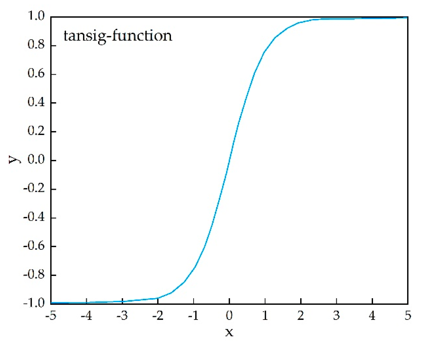
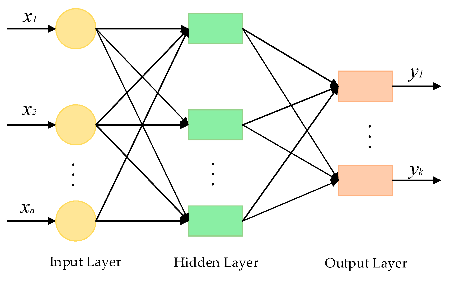
2. BP Neural Network

In 1986, Rumelhart and McClelland first proposed the BP Neural Network (BPNN) [15,16,17], which is a multilayer feedforward neural network based on error back propagation. The BPNN is widely used to deal with nonlinear problems [18,19] due to the characteristics of self-adaptation and self-learning. The BPNN can be divided in two ways: signal forward propagation and error backward propagation. When the signal propagates in the forward direction, the signal propagates from the output layer to the output layer; when the error propagates backward, the error propagates back to each layer. The structure of BPNN is divided into three layers: input layer, hidden layer and output layer, which is shown in Figure 5. The number of hidden layer nodes is a very important parameter, and its setting has a great impact on the performance of BPNN [20] The determination of the number of hidden layer nodes is still one of the most difficult problems for BPNN [21]. At present there is no good solution, and the optimal number can only be determined by experimental methods.

The BPNN hidden layer function is one that runs on the neurons of the artificial neural network and is responsible for mapping the input of the hidden layer to the output. The hidden layer function introduces nonlinear factors into the neural network, so that BPNN can approximate any nonlinear function and apply it to more nonlinear models. The BPNN output layer commonly used linear functions; the commonly used functions of the hidden layer are the logsig function and the tansig function, the expressions of which are shown in Equations (1) and (2), respectively [22].

$$y=\frac{1}{1+e^{-x}}$$

(1)

$$y=\frac{1-e^{-x}}{1+e^{-x}}$$

(2)

where x is the independent variable, and j is the dependent variable.

The input value of Logsig function and Tansig function can take any value, and the range of the output value is (0,1) and (−1,1), respectively. The image of the logsig function and tansig function is as shown in Figure 6 and Figure 7, respectively.

The BPNN continuously adjusts the value of weight and threshold by back propagating the calculation error [23], finally making the error of the overall prediction result reach the ideal situation and achieving the infinite approximation of any nonlinear function [24]. In the oilfield development index prediction process, the work of BPNN is mainly divided into the learning phase and the prediction phase. The learning phase is mainly to input the sample data of the oilfield for independently learning to determine the threshold and connection weights of the network, while the prediction phase mainly uses a well-trained neural work to predict simulation results corresponding to unknown data [25]. The calculation process of BPNN is as follows: analyze the error between the output results and the actual results. If the error does not meet the expected requirements, the error will propagate back along the original path to correct the ownership value and threshold, so that the error calculated by the next forward propagation is closer to the expected requirements [26]. Through repeated training, adjust the weight and threshold of BPNN, and finally make the error stable.

Sun et al. [27] established an oilfield single-well production prediction model by BPNN, and their results showed that the error of the transfer function to the tansig function was less than that of the logsig function when the remaining parameters were unchanged. Sun et al. used the monthly oil production of a single well as a learning sample for training to predict the monthly production of a single well, and the errors of the training samples and prediction samples were 4.39% and 0.263%, respectively. Therefore, this proves the feasibility of BPNN in solving the complex nonlinear problem of predicting oilfield development indicators.

BPNN has been widely used in oilfield seismic and logging and to solve the complex nonlinear problems between oilfield development index prediction and its multiple influencing factors. However, with the in-depth study of its functions, its shortcomings have gradually emerged, such as: it easily falls into a local minimum, it has slow convergence, low prediction accuracy, etc. In view of the above shortcomings, many scholars propose to use different intelligent algorithms combined with BPNN to achieve optimization.

For example, Tian et al. [28] used a genetic algorithm (GA) to optimize BPNN, and GA-BPNN was used to predict shale gas production. The maximum relative error of the prediction results was reduced from 17.821% to 8.184%, This shows that GA-BPNN not only overcomes the defect that BPNN is easy to fall into local minimum, but also reduces training time and improves prediction accuracy. Due to the probability of crossover and mutation of genetic algorithm is constant, it is difficult for GA to get rid of the limitation of local optimum and hinders the convergence speed of the algorithm. Srinivas et al. [29] proposed an adaptive genetic algorithm (AGA) to adjust the probability of crossover and mutation according to the fitness value in response to the above problems. However, AGA will make individuals with higher evolutionary degrees lose evolution opportunities in the early stages of evolution, leading to population evolution. Su et al. [30] used an improved adaptive genetic algorithm (IAGA) combined with BPNN to optimize, and compared the training results with the actual value and the fitness values before and after the improvement, and found that IAGA-BPNN improves the accuracy of the training results by a large margin and that the convergence speed is faster.

Aiming at the problem that BPNN has high initialization sensitivity and that it easily falls into local minimum, Qin et al. [31] proposed a hierarchical fusion optimization model (MB-PSO-CS-BP), which refers to the use of the Mini-Batch algorithm in the lower layer to divide the particle swarm into small groups, and then the particle swarm optimization algorithm (MB-PSO) is used for local search. On this basis, the cuckoo search algorithm (CS) is used for global search, thereby reducing the sensitivity of BPNN initialization and alleviating its symptoms of falling into local minimum. Through the example verification of the proposed algorithm with actual data, it is found that compared with the PSO-BP model and the cs-bp model, the mb-pso-cs-bp fusion model has improved in many indexes, such as mean square error and global optimal value, which improves the accuracy and stability of BPNN prediction.

After the intelligent algorithm is combined with BPNN, each individual vector of various intelligent algorithms contains n elements.

$$n=(a+1)\times b+(b+1)\times c$$

(3)

where a is the number of input layer nodes; b is the number of hidden layer nodes; c is the number of output layer nodes.

BPNN provides a good idea for solving the complex non-linear problem of oilfield development index prediction, and the prediction effect of BPNN after intelligent algorithm optimization is better. Although the prediction accuracy of the BPNN optimized by the intelligent algorithm is improved, the initialized weights and thresholds are also random when the intelligent algorithm starts to optimize the weights and thresholds. In addition, there are many results caused by the matching of many weights and thresholds, resulting in large fluctuations in the final error prediction results.

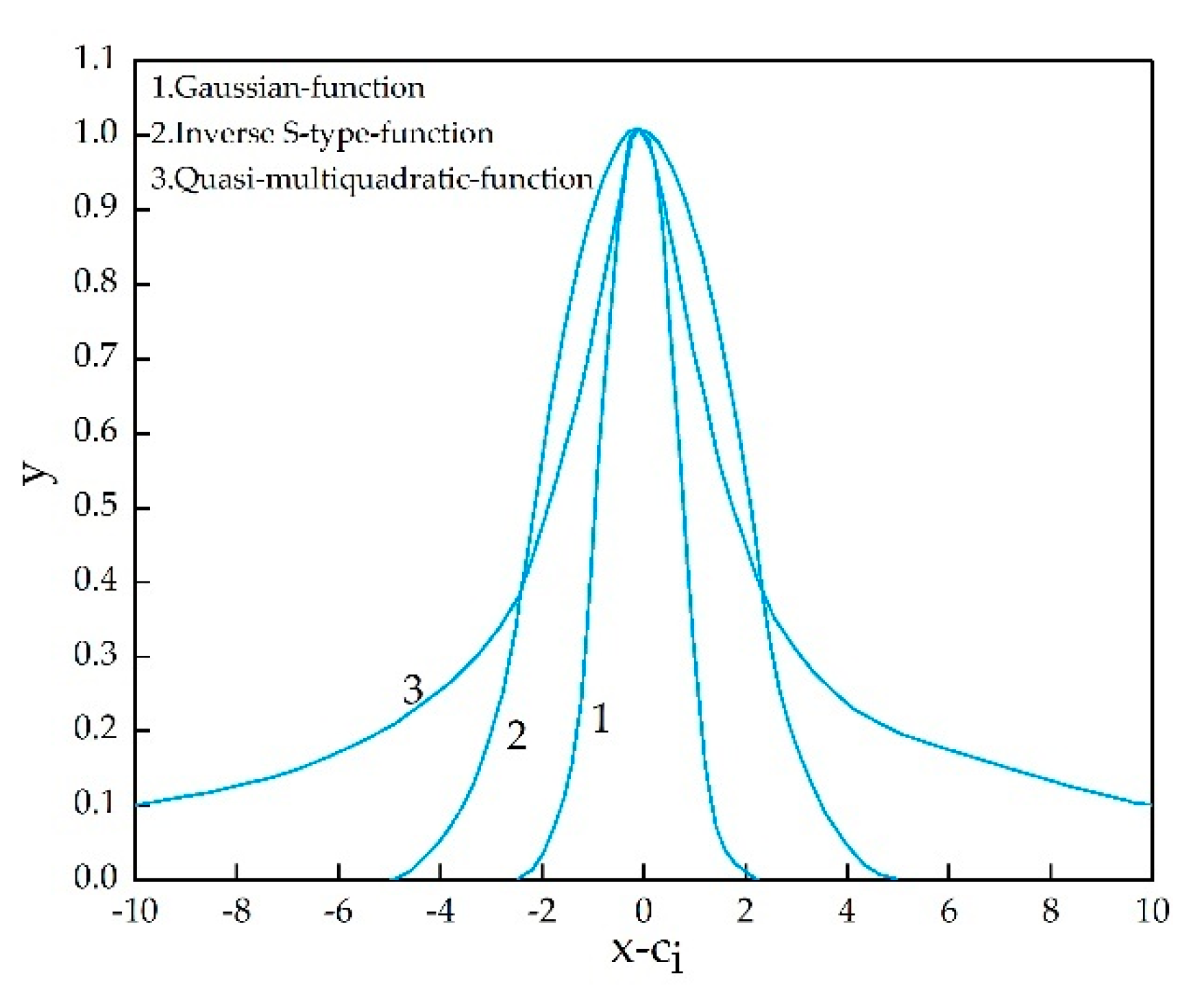
3. Radial Basis Function Neural Network

In 1988, Moody and Darken proposed a radial basis function neural network (RBFNN) based on radial basis function (RBF). Compared with other feedforward ANNs, RBFNN, which is an efficient feedforward Ann, has global optimal characteristics, optimal approximation performance [32], fast convergence speed, simple learning and easy implementation [33]. Although the transformation of input variables of RBFNN from input layer space to hidden layer space is nonlinear, the mapping from hidden layer space to output layer space is linear. This is the reason why is the output of RBFNN is the linear weighted sum of the hidden layer output. The role of the RBFNN hidden layer is to map the vector from low dimension to high dimension, so that the low dimension is linearly inseparable from the high dimension and becomes linearly separable, mainly using the idea of kernel function. The mapping of RBFNN from input to output is non-linear, while the network output is linear to the adjustable parameters. In this way, the weight of the network can be directly solved by linear equations, which greatly speeds up the learning speed and avoids the problem of local minima. The network structure of RBFNN can be divided into three layers: input layer, hidden layer (only one), and output layer [34]. Its structure is shown in Figure 8.

The typical radial basis functions (basis functions) of the RBFNN hidden layer are Gaussian function, inverse S-type function and quasi-multiquadratic function, and the expressions are shown in Equations (4)–(6) respectively. The common function of RBFNN hidden layer is Gaussian function (Equation (4)).

$$y=\exp \left(-\frac{{\Vert x-c_i\Vert }^2}{2{\delta }_i{}^2}\right),i=1,2,\cdots n.$$

(4)

$$y=\frac{1}{1+\exp \left(\frac{{\Vert x-c_i\Vert }^2}{2{\delta }_i{}^2}\right)},i=1,2,\cdots n.$$

(5)

$$y=\left(\frac{1}{{\left({\Vert x-c_i\Vert }^2+{\delta }_i{}^2\right)}^{1/2}}\right),i=1,2,\cdots n.$$

(6)

where x is the input vector, n-dimensional, c_i is the center vector of the i-th basis function, n-dimensional; ‖x − c_i‖ is the Euclidean distance between vector x and vector c_i; δ_i is the width of the i-th basis function.

The Gaussian function, Inverse S-type function and quasi-multi-quadratic function are respectively shown in Figure 9. If the width δ_i of the radial basis function is smaller, the basis function is more selective.

The idea of RBFNN is to use the radial basis function as the “base” to form the hidden layer space, so that the input vector can be directly mapped to the hidden layer space without connecting weights. When the center point and mean square error of the RBFNN are determined, the mapping relationship between the input vector and the hidden layer space is also determined. RBFNN does not have a back-propagation process similar to BPNN, so compared to BPNN, not only is the calculation process simple [35], but also the calculation speed is faster. Based on these characteristics, many scholars began to study and research RBFNN in depth.

Xu et al. [36] used RBFNN to establish a development index prediction model with seven influencing factors, such as remaining geological reserves and total number of production wells as input, and monthly oil and liquid production as output. The prediction results show that the average relative errors of RBFNN’s prediction of monthly oil production and liquid production are 1.47% and 0.42%, respectively, which demonstrates the feasibility of RBFNN in solving the complex non-linear problem of oilfield development index prediction.

In view of the difficulty in determining the center and width of the RBFNN basis function, Liu et al. [37] applied the immune principle (IP) to optimize the center and width of the RBFNN basis function and established a prediction model with 13 parameters such as water cut and average daily output of 42 fractured wells in the Zhongyuan Oilfield as input and productivity as output. The complex non-linear relationship between input samples and output samples is studied. The data of 35 wells are used for training, and the data of the remaining seven wells are used to verify the model. The results show that the prediction model based on IP-RBFNN has a small amount of calculation, high accuracy, and the relative error is less than 7%. Shao et al. [38] combined the principal component analysis (PCA) with RBFNN to improve the performance and robustness of the RBFNN model. PCA can greatly reduce the dimensionality of the dimensionality input parameters and reduce the complexity of the RBFNN mapping function. Compared with a single RBFNN, PCA-RBFNN not only reduces the computational complexity, but also improves the prediction accuracy. Xie et al. [39] proposed an improved second-order algorithm (ISO) for training radial basis function networks (RBFNN). The ISO algorithm takes advantage of the fast convergence speed and strong search ability of the second-order algorithm, can use fewer RBF units to achieve smaller training and test errors. The ISO algorithm optimization principle is to obtain more accurate prediction results by increasing variable dimensions. Only one Jacobian row is stored and used for multiplication, rather than the entire Jacobian matrix storage and multiplication. Therefore, reducing memory is beneficial to calculation speed and can be used to deal with problems with an unlimited number of patterns.

Compared with the widely used BPNN, Zhang et al. [40] proved that the approximation effect of RBFNN in nonlinear functions is better through an example analysis, and can basically achieve a complete approximation. For the prediction of certain oilfield development indicators, RBFNN has faster training speed and fewer iterations, and is more suitable for complex systems with unknown parameters.

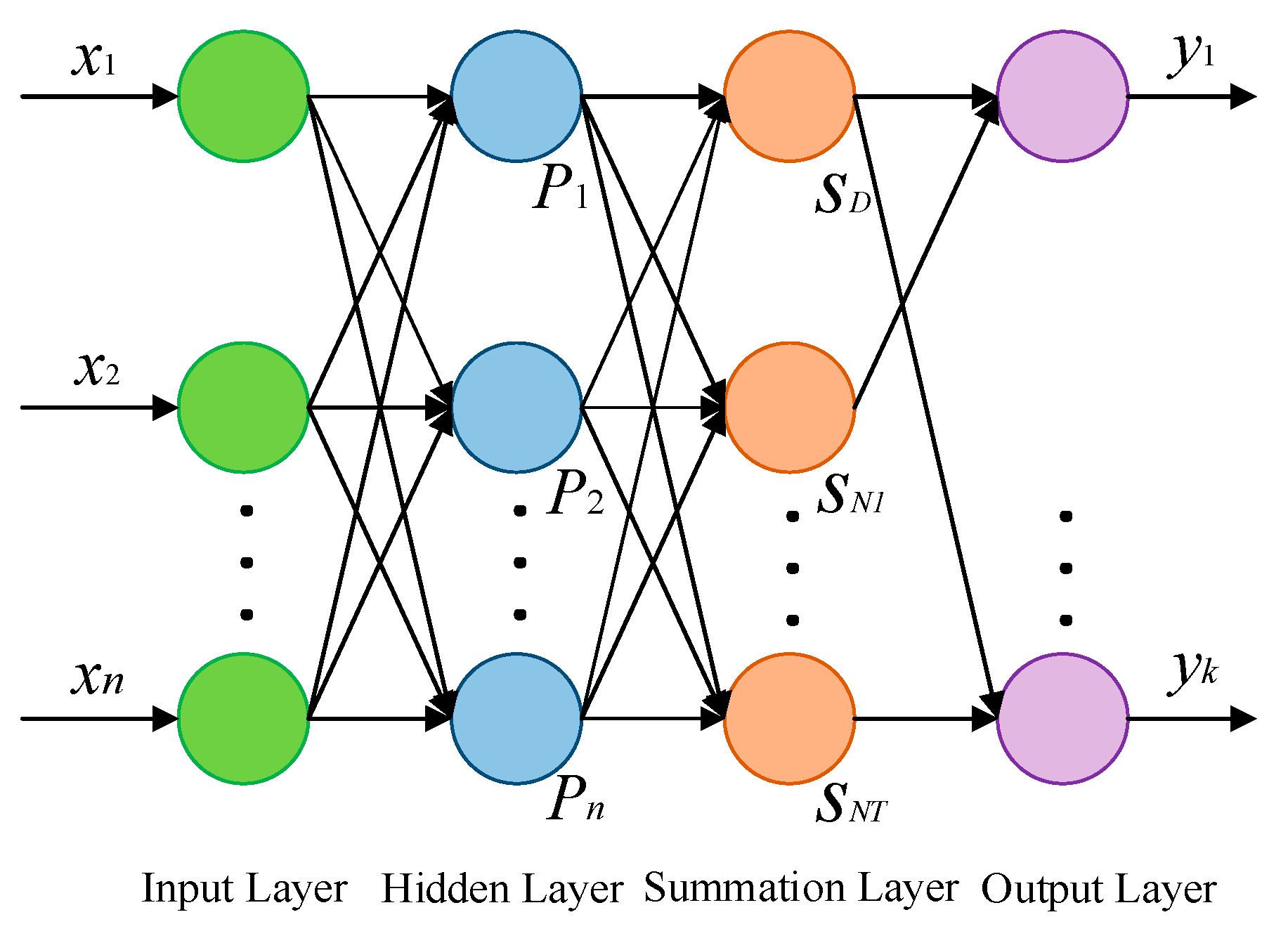
4. Generalized Regression Neural Network

In 1991, Donald proposed the Generalized Regression Neural Network (GRNN) [41], which is an improved form of RBFNN and is based on regression mathematical statistics. GRNN has strong non-linear mapping ability and learning speed, and has stronger advantages than RBFNN. It is the final convergence of the network to an optimized regression with a large number of samples. When the sample data is small, the prediction effect is better. In addition, unstable data can also be handled. The network structure of GRNN is four layers, which adds a summation layer to the network structure of RNFNN. It’s network structure is shown in Figure 10.

The number of nodes in the GRNN input layer is equal to the dimension of input vectors in learning samples, and the number of nodes in the hidden layer is equal to the number n of learning samples. The output of input layer node i is in exponential form of exponential square D_i² = (x − x_i)^T(x − x_i) of Euclid distance square between input variable and its corresponding sample x. The hidden layer function is:

$$P_i=\exp \left[-\frac{{\left(x-x_i\right)}^T\left(x-x_i\right)}{2{\delta }^2}\right],i=1,2\cdots n.$$

(7)

where x is the network input variable and x_i is the learning sample corresponding to the i node.

The summation layer uses two types of functions to sum. The first type of function arithmetically sums the outputs of all hidden layer nodes, and the connection weight between the hidden layer and each node is one; Another kind of function performs weighted summation on the nodes of all hidden layers. The summation layer is divided into two parts, which are functions S_D and S_Nj, and the expressions are:

$$S_D={\displaystyle \sum _{i=1}^n\exp \left[-\frac{{\left(x-x_i\right)}^T\left(x-x_i\right)}{2{\delta }^2}\right]}={\displaystyle \sum _{i=1}^n{P}_i},i=1,2\cdots n.$$

(8)

$$S_{Nj}={\displaystyle \sum _{i=1}^n{y}_{ji}\exp \left[-\frac{{\left(x-x_i\right)}^T\left(x-x_i\right)}{2{\delta }^2}\right]}={\displaystyle \sum _{i=1}^n{y}_{ji}{P}_i},j=1,2\cdots k.$$

(9)

where P_i is the output of the hidden layer, n is the number of learning samples, k is the dimension of the output vector, and y_ji is the value of the j-th learning sample corresponding to the output vector.

The number of nodes in the output layer is equal to the dimension k of the output vector in the learning sample. Each node divides the output of the summation layer, and the expression of the prediction result y_j output by the node j is:

$$y_j=\frac{S_{Nj}}{S_D},j=1,2\cdots k.$$

(10)

The theoretical basis of GRNN is nonlinear regression analysis. The input variables of the input layer are directly transmitted to the hidden layer, and then transmitted to the summation layer through the activation of the function of the hidden layer. The summation layer uses two kinds of functions to sum, and these are then transmitted to the output layer. Each node of the output layer divides the output of the summation layer in turn and outputs the corresponding prediction results. Based on the simpler calculation process and structure of GRNN, many scholars have carried out extensive research and applications on it.

Chen et al. [42] proposed to use GRNN for nonlinear optimization regression analysis. By comparing the development modes and development effects of similar oilfields, a prediction model was established to predict the development indexes of new oilfields. Eleven factors affecting the development indexes, such as oil-bearing area and permeability, were selected as input variables to predict the development indexes such as recovery ratio and well pattern density. The prediction results show that GRNN has strong nonlinear mapping ability and good stability, and can solve the problems of prediction and development strategy of new oilfield development indexes. Chen et al. [43] proposed to establish a prediction model of oil well water cut by using GRNN, and the prediction results showed that the maximum relative error was 6.32%. By comparing the fitting results of GRNN and BPNN, it can be found that when there are few sample data, the fitting results of GRNN are closer to the measured values, and the relative error is smaller, which fully shows that GRNN has great advantages in oil well water cut prediction.

In order to further improve the prediction accuracy of GRNN, it is considered to optimize GRNN combined with various intelligent algorithms. The idea of optimization is to optimize the unknown weight, translation factor and other parameters in the model.

Huang [44] et al. proposed GRNN based on genetic algorithm (GA) optimization to solve the problem of out-of-sample expansion. GA has a good global search ability, and as the population size continues to increase, GA can obtain a better smoothing factor in a wider search space. The prediction results show that GA-GRNN has higher prediction accuracy than the improved generalized regression neural network (IGRNN). The essence of GA optimization is to determine the optimal smoothing factor of GRNN, and its optimized form is used to predict the low-dimensional embedding of test samples. The fruit fly optimization algorithm (FOA) was proposed by Taiwanese scholar Pan in 2011 [45]; it is a new method for seeking global optimization based on fruit fly foraging. Liu et al. [46] proposed to use an improved Drosophila optimization algorithm (IFOA) to optimize GRNN, which was predicted by the GRNN model, the FOA-GRNN model and the IFOA-GRNN model, respectively. The maximum relative errors of predicted results by GRNN and FOA-GRNN were 10.92% and 13.45%, respectively, while the maximum relative errors of IFOA-GRNN were only 6.80% By comparing the prediction results of three prediction models, it is found that IFOA-GRNN has faster convergence speed, better nonlinear fitting ability and higher prediction accuracy. Ding et al. [47] proposed a non-dominated sorting genetic algorithm (NSGA) to optimize GRNN’s elite strategy integration model to predict and optimize the quality characteristics of fiber laser cutting stainless steel and to take laser power, cutting speed, air pressure, defocus, etc. as input variables, and cut width and surface roughness as output variables to generate the data set of the model. In the NSGA-GRNN model, the cross-validation method is used to train the network to obtain the best GRNN prediction model. The relative error of the NSGA-GRNN prediction model is controlled within +/−5%. This model can be used to characterize the process parameters of fiber laser cutting stainless steel in detail.

GRNN has the characteristics of a simple calculation process, a fast learning speed, less adjustment parameters, good global convergence, and so on. Compared with BPNN, GRNN can achieve better prediction results in dealing with nonlinear problems with small samples [48]. GRNN, as an improved ANN of RBFNN, is superior in dealing with nonlinear problems in theory, and can minimize the influence of subjective factors on approximation results Compared with RBFNN, GRNN is characterized by simple learning process: unknown variables in RBFNN include function center c, function width δ and weight ω; However, GRNN regards the learning sample as function center c, cancels weight ω, and only retains an unknown variable-function width δ. Therefore, intelligent algorithms (such as GA, PSO, FOA, etc.) are easier to combine with GRNN, and only need to adjust one parameter δ to make the prediction result more accurate.

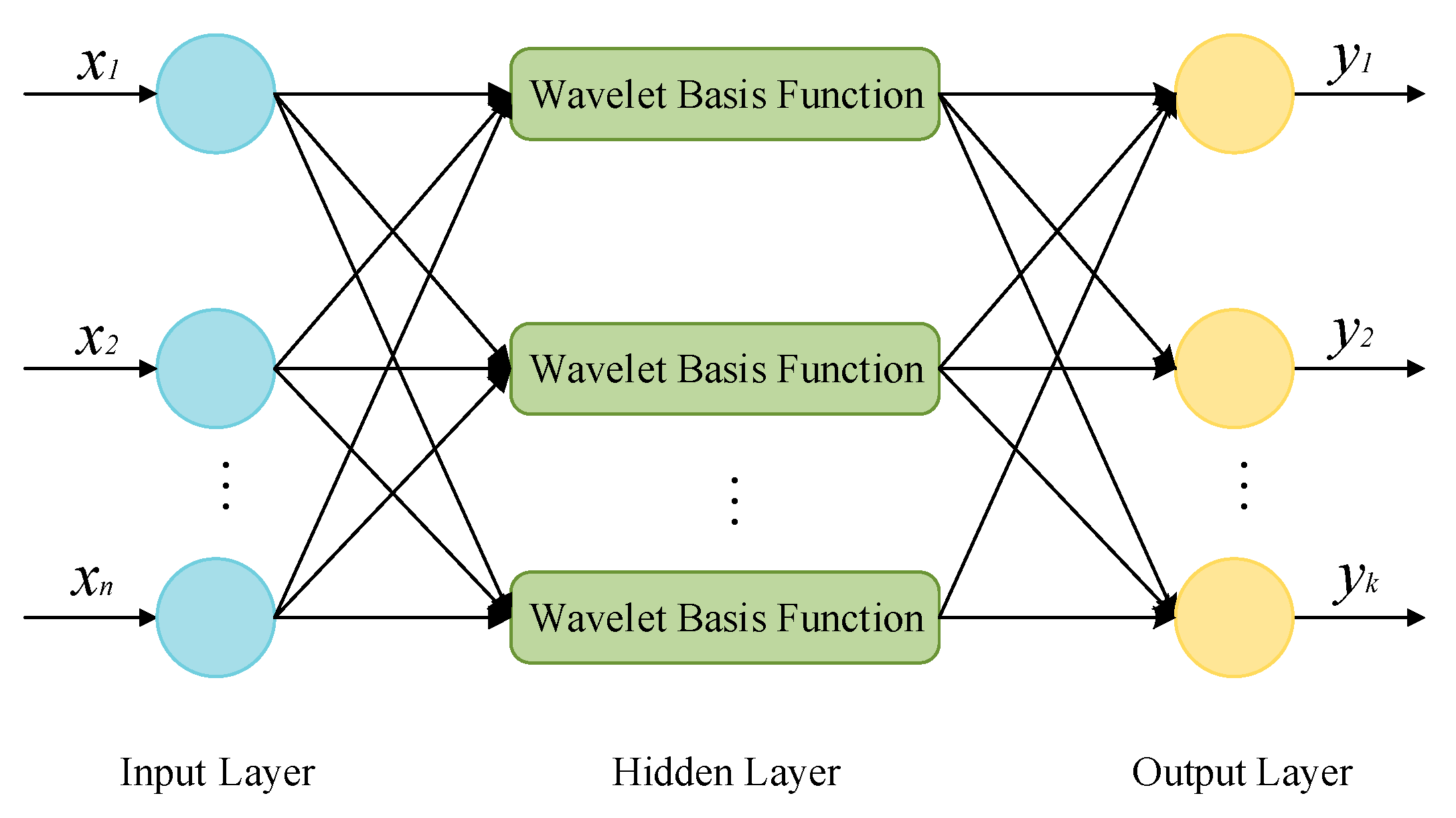
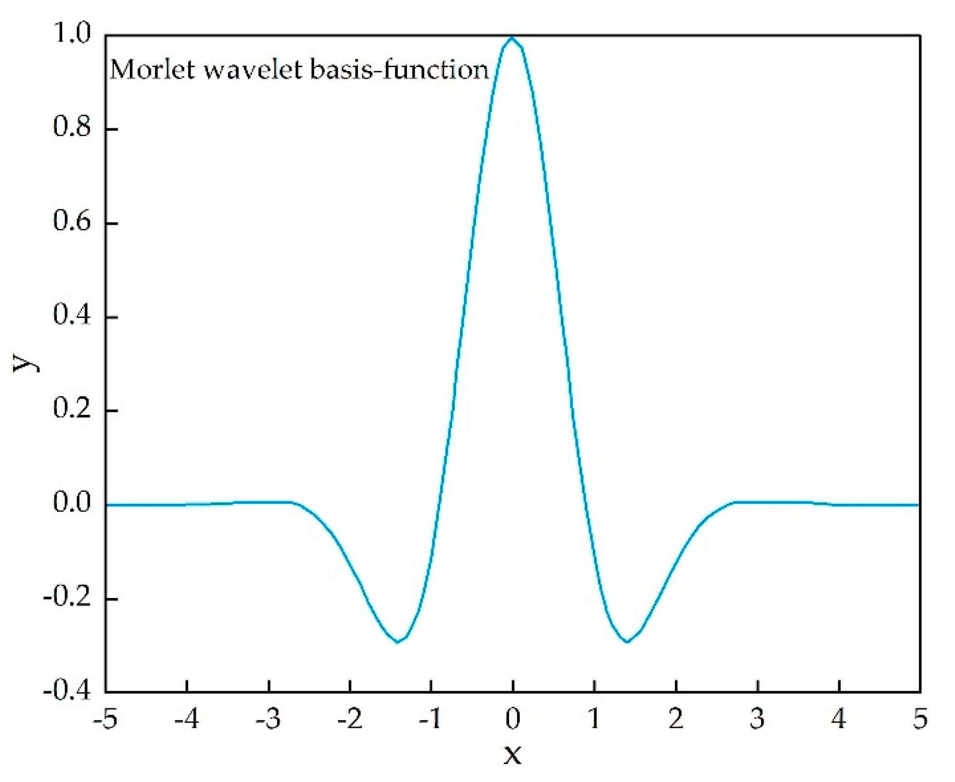
5. Wavelet Neural Network

In 1992, Zhang and Albert Benveniste first proposed Wavelet Neural Network (WNN) [49], which is an artificial neural network derived from wavelet transformation based on the BPNN structure [50]. WNN uses the wavelet function to replace the node function of the hidden layer of the conventional neural network, and the corresponding connection weight from the input layer to the hidden layer and the threshold of the hidden layer are replaced by the scale and translation parameters of the wavelet function; that is, the activation function is the located wavelet basis function. WNN’s basic idea and principle is to take the index attribute value of the characteristics of the evaluation object as the input vector of the neural network and the known corresponding evaluation value as the WNN’s output. It can be trained by batch processing through the conjugate gradient method to adaptively adjust the wavelet coefficients and network weights. By learning enough samples to train the network, WNN is like a “black box”, storing expert evaluation experience and some mathematical reasoning mechanisms, and establishing a non-linear mapping relationship from the evaluation index attribute value to the output comprehensive evaluation value. In this way, the trained wavelet neural network can be used to evaluate new evaluation objects. Its network structure is shown in Figure 11.

WNN is different from BPNN in that one is the calculation function of the hidden layer output while the other is that the calculation process discards the threshold and only retains the weight. The hidden layer of WNN often uses Morlet wavelet basis functions, and the calculation process of the hidden layer output is:

$$h_j=h\left(\frac{{\displaystyle \sum _{i=1}^n{w}_{ij}{x}_i-b_j}}{a_{ij}}\right),j=1,2,\cdots ,l.$$

(11)

where $h_j$ is the output of the $j$-th node of the hidden layer; $h$ is the Morlet wavelet basis function; $w_{ij}$ is the connection weight from the $i$-th node of the input layer to the $j$-th node of the hidden layer; $x_i$ is the input of the $i$-th node of the input layer; $b_j$ is the translation factor of the $j$-th node of the hidden layer; $a_j$ is the expansion factor of the $j$-th node in the hidden layer; $n$ is the number of nodes in the input layer; $l$ is the number of nodes in the hidden layer.

WNN constructed by Morlet wavelets ($r$ is usually 1.75) have been used widely in various fields. The expression of the Morlet wavelet basis function in the above Equation (11) is:

$$h=\cos (1.75x)e^{-x^2/2}$$

(12)

The advantage of Morlet wavelet basis is that the function expression is simple and symmetrically distributed, but the disadvantage is that the signal after decomposition cannot be reconstructed. The image of the Morlet wavelet basis function is shown in Figure 12.

Combining the strong robustness of ANN with the good time-frequency local characteristics of wavelet transform and the multi-resolution function can reduce the probability of the model falling into the local extreme value and strengthen the generalization ability, so it has better approximation and fault tolerance [51]. Therefore, based on the fact that WNN has a better predictive effect than BPNN in dealing with nonlinear problems, many scholars have carried out more in-depth research, application and improvement on it.

Li et al. [52] proposed to use WNN to predict annual oil production using the actual production situation of the oilfield to establish a prediction model with six influencing factors such as water cut and annual recovery, etc, as input variables, and annual oil production as output variables, and the prediction results show that the maximum relative error of WNN’s forecast of annual oil production is only 2.96%. Li et al. [53] selected seven factors affecting development indicators such as formation pressure, remaining recoverable reserves, number of oil wells opened and injection production ratio as the input variables of WNN. The network model structure is determined as 7-6-4, and the network output is predicted with oil production, water production, recovery degree and water content. Through the continuous learning and training of the network, the past experience and acquired expert knowledge are accumulated into the network structure, and the error is analyzed after comparing the predicted result with the actual value. Next, the network parameters are adjusted, and the predicted result shows that the predicted value and actual value of the maximum relative error of the value is 4.57%. This shows that WNN has high accuracy in oilfield development performance index prediction; at the same time, it also shows that the use of WNN to predict the oilfield development dynamic indices is correct and feasible.

In order to further reduce the probability of WNN falling into local extremum and improve the accuracy of prediction, various intelligent algorithms can also be considered to optimize it. The idea of optimization is also to optimize the unknown parameters in the model (such as weights, translation factors, and expansion factors). Liu et al. [54] proposed a wavelet neural network forecasting oil price model (SA-WNN) based on sentiment analysis (SA). Firstly, the emotion analysis method is used to preprocess the text data. Next the market trend item was calculated based on the preprocessing results, and then the item was used as the input data of WNN. The prediction results show that compared to the traditional BP neural network model and the independent source analysis-based wavelet neural network (ICA-WNN) model, the SA-WNN model can more accurately predict the directional trend of oil prices. Chen et al. [55] established the artificial bee colony algorithm (ABC) to optimize the wavelet neural network prediction model (ABC-WNN), and compared the prediction results with the prediction results of BPNN and WNN, and the prediction results are sorted from high to low: ABC-WNN, WNN, BP. Zheng et al. [56] improved on the leapfrog algorithm (SFLA) and proposed the ISFLA-WNN model, whose prediction results are closer to the true value than SFLA-WNN and have higher accuracy in dealing with nonlinear problems. Like the above three ANNs, intelligent algorithms (such as SA, ABC, SFLA, etc.) can also be combined with WNN to make the prediction results more accurate.

Compared with BPNN, WNN has great improvements in convergence speed, generalization ability and approximation accuracy, but it still has problems such as being trapped in extreme values and network stability. WNN avoids the blindness of BP neural network structure design and non-linear optimization problems such as local optimization, greatly simplifies training, has strong function learning ability and promotion ability and broad application prospects. With the continuous deepening of WNN research, its application fields will become more and more extensive, but because it has just started, there are still drawbacks: the number of hidden layer nodes is difficult to determine, fault tolerance, convergence, generalization and computational complexity or lack of theoretical support, and how to select the appropriate wavelet function to obtain the best prediction results in different nonlinear practical problems need to be resolved.

6. Establishing the Experimental Model of Oilfield Development Index Prediction

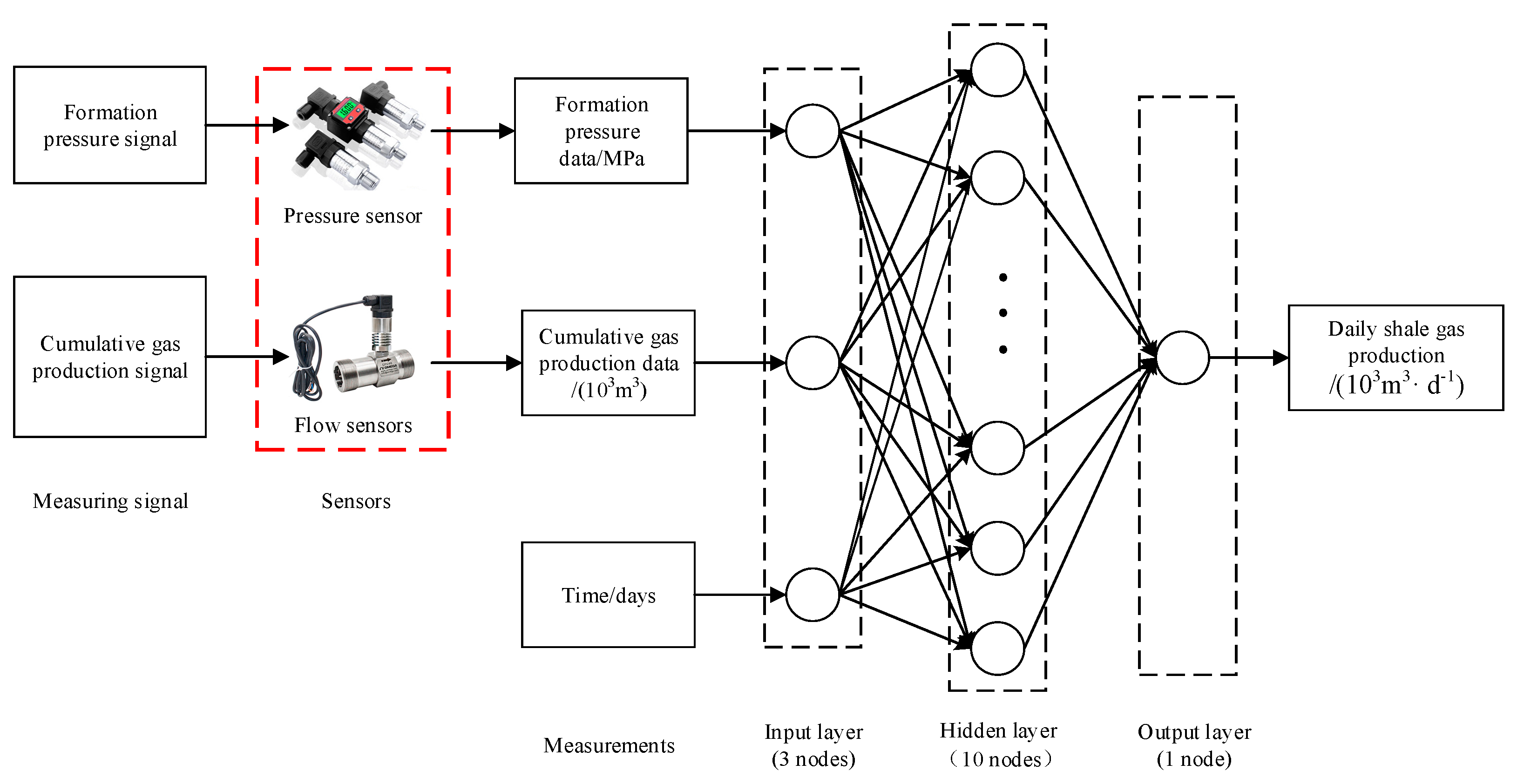
6.1. Establish Experimental Model

According to the single-well production data of Haynesville in the United States [28], this paper uses Matlab software, adopts a three-layer network structure of BPNN, and uses the Whale Optimization Algorithm (WOA) to optimize BPNN’s inter-layer weights and intra-layer thresholds (WOA-BPNN) in order to establish a decline model for predicting daily shale gas production.

With the gradual decrease in formation pressure, the fractures in the shale will be closed, resulting in a decrease in the permeability of the shale, therefore affecting the gas flow in the shale reservoir and resulting in a decrease in production. The cumulative gas production can reflect the actual natural energy of the shale formation. As the cumulative gas production increases, the actual natural energy of the shale formation will decrease, and the gas supply capacity of the shale gas reservoir will decrease, resulting in a decrease in gas production. According to the classic Arps decline model, the gas production is a function of time. Therefore, based on the above analysis, select formation pressure, cumulative gas production, and time as three input variables of ANN, and the daily production of shale gas as the output variable of ANN. At the same time, WOA should be used to optimize the weights and thresholds of BPNN in order to establish an ANN prediction page. The experimental model of daily rock gas production is shown in Figure 13.

This experimental model takes formation pressure, cumulative gas production and time as input variables [57], and shale gas daily output as the output prediction model. The pressure sensor is needed to measure the formation pressure signal, which converts the formation pressure signal into the formation pressure value, and takes the formation pressure data as the input variable of the model [58,59,60,61]. Similarly, the measured cumulative gas production signal needs a flow sensor, which converts the cumulative gas production signal into the cumulative gas production value and takes the cumulative gas production data as the input variable of the model [62,63,64,65,66].

6.2. Learning Sample Data

Selecting the daily production data of a well in the Haynesville shale gas field in the United States, and analyzing the daily production of shale gas under different formation pressures, cumulative gas production and time, the corresponding WOA-BP prediction model was established. Twenty-eight learning samples were selected for daily shale gas production under different conditions, and the last five data were not included in the learning, as the prediction model accuracy test, as shown in

Table 1. Basic data of ANN learning training samples [28].

Sample	Time/(d)	Cumulative Gas Production/(103m3)	Formation Pressure/(MPa)	Actual Daily Shale Gas Production/(103m3·d−1)
1	1	15.779	29.575	15.779
2	19	50.316	27.501	13.875
3	49	91.090	23.353	14.730
4	79	116.248	20.894	9.988
5	108	140.539	18.590	8.317
6	140	158.757	17.054	7.190
7	170	172.637	15.440	6.413
8	203	186.518	14.134	5.752
9	232	197.795	12.829	5.286
10	263	208.206	11.830	4.897
11	324	227.291	10.063	4.314
12	354	236.834	9.141	3.848
13	382	242.907	8.527	3.614
14	414	252.450	7.835	3.381
15	445	258.522	7.221	3.148
16	475	267.197	6.530	2.993
17	506	273.270	5.915	2.837
18	535	281.078	5.337	2.682
19	565	285.417	4.916	2.410
20	595	292.357	4.532	2.410
21	629	298.428	4.148	2.254
22	659	303.632	3.764	2.176
23	689	312.308	3.150	2.060
24	712	318.312	2.842	2.060
25	730	321.851	2.689	1.943
26	746	323.587	2.689	1.943
27	760	327.055	2.458	1.866
28	774	329.661	2.228	1.904
Test	791	331.393	2.074	1.788
Test	805	335.731	1.920	1.788
Test	820	337.467	1.767	1.671
Test	833	340.069	1.613	1.671
Test	850	342.672	1.383	1.593

Notes: The data in Table 1: Sourced from “Chinese Science and Technology Papers”, received date: 6 July 2016, authors: Yapeng T. and Binshan J., website: https://kns.cnki.net/kns8/defaultresult/index, accessed on 14 September 2021.

.

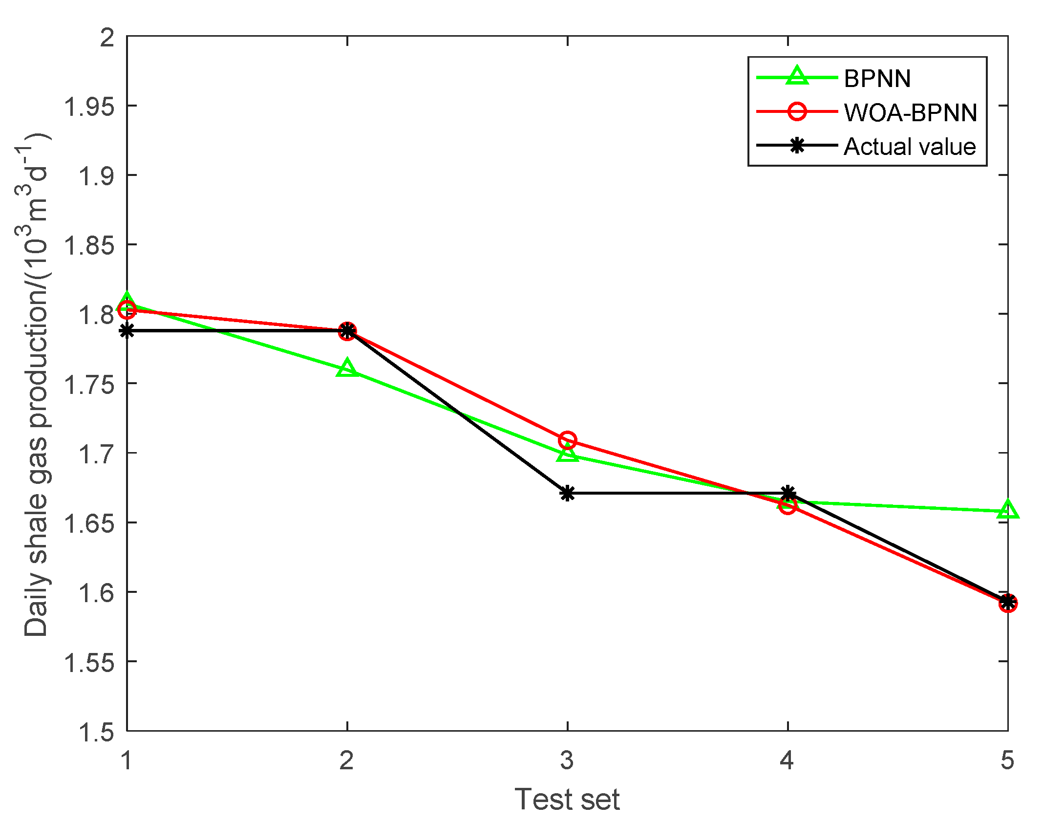
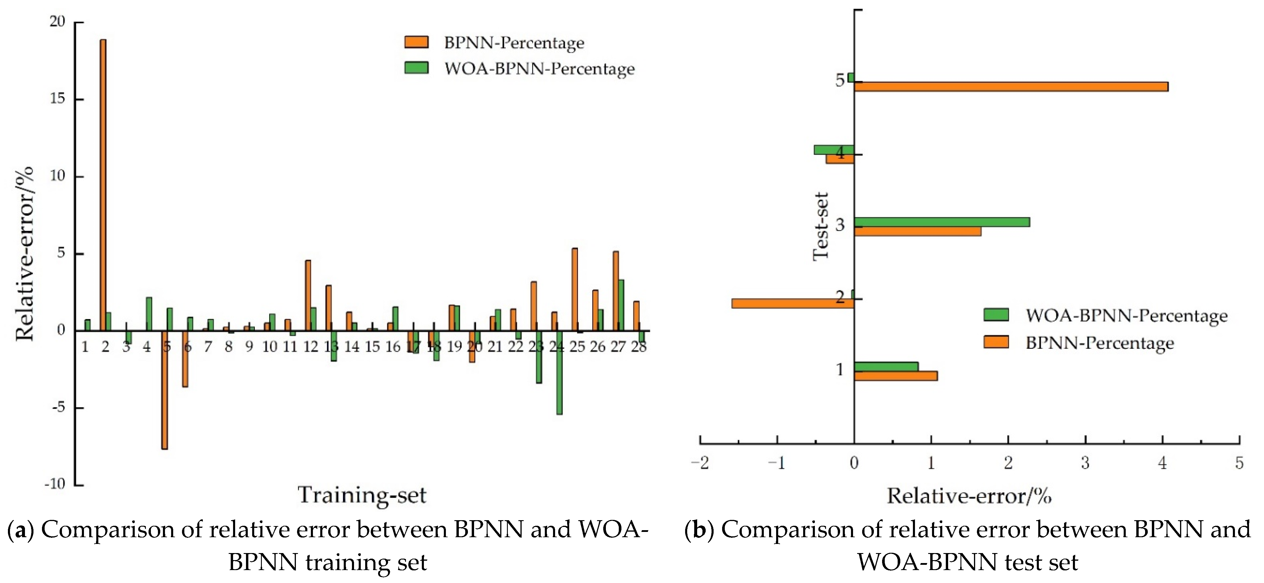
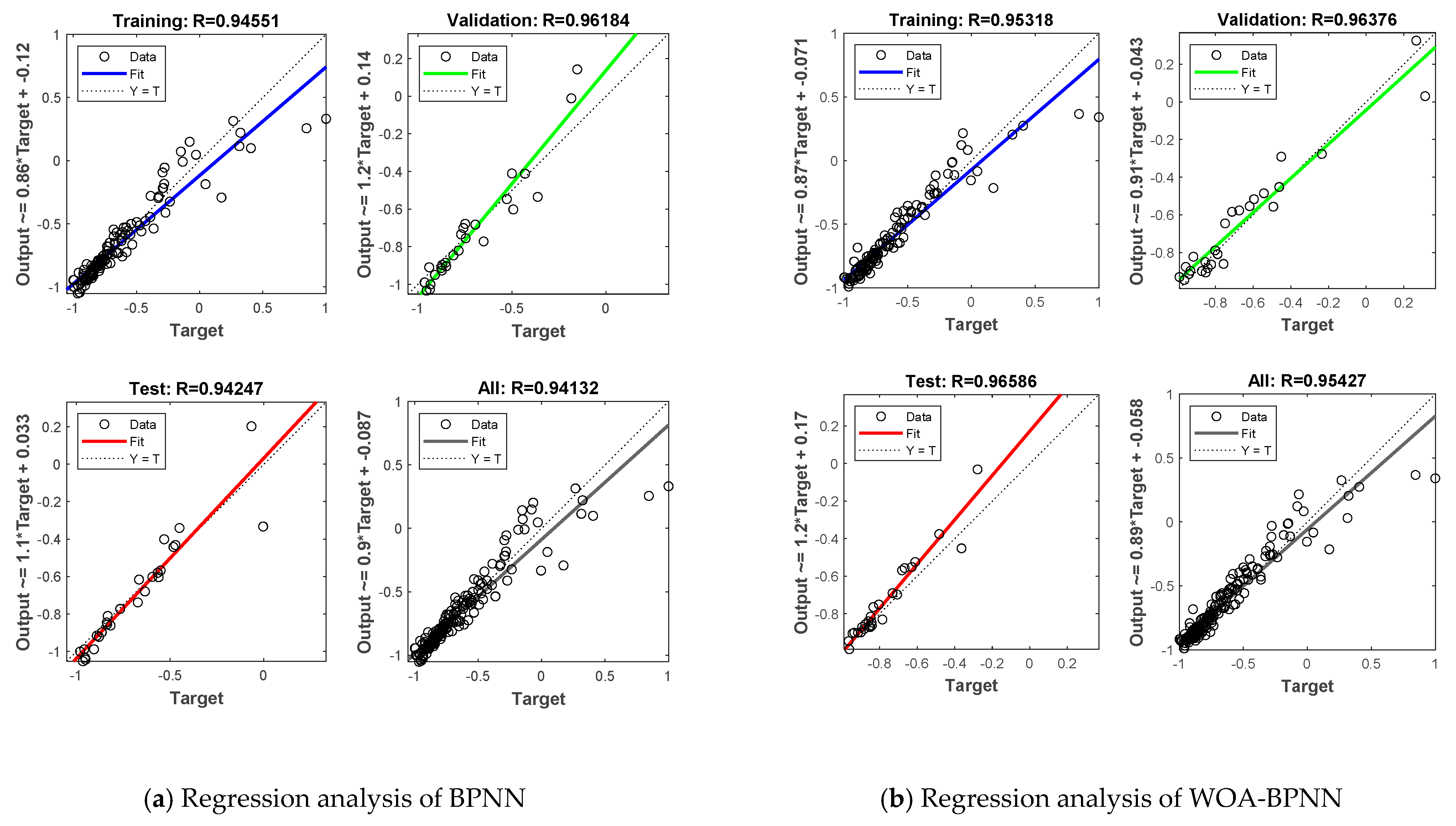
6.3. Analysis of Prediction Results

Using Matlab software for calculation, the comparative results of conventional BPNN and WOA-BPNN training value and actual data are shown in Figure 14a,b (28 training data). Figure 15 shows the comparison result of the actual value, BPNN predicted value and WOA-BPNN predicted value (5 predicted-data). Figure 16a is the comparison result of the relative error between the BPNN training value and the WOA-BPNN training value. Figure 16b shows the comparison of the relative error between the predicted value of BPNN and the predicted value of WOA-BPNN. Figure 17a,b are the comparison results of the correlation between BPNN and WOA-BPNN training set, prediction set and actual value, respectively.

Mean relative error (MRE) [67] and root mean square error (RMSE) [68,69] were chosen as the evaluation criteria. The specific calculation formulas are as follows (13) and (14):

$$MRE=\frac{1}{N}{\displaystyle \sum _{i=1}^N\left|\frac{y^{\prime }-y}{y}\right|}$$

(13)

$$RMSE=\sqrt{\frac{1}{N}{\displaystyle \sum _{i=1}^N{\left(y^{\prime }-y\right)}^2}}$$

(14)

where y’ is the daily production value of shale gas predicted by ANN, and y is the actual daily production value of shale gas.

The error results of BPNN and WOA-BPNN in predicting daily shale gas production are shown in

Table 2. Comparison of prediction errors between BPNN and WOA-BPNN.

ANNs’ Name	MRE/%	RMSE/%
BPNN	0.972	0.035
WOA-BPNN	0.496	0.017

below.

The Whale Optimization Algorithm (WOA) optimizes BPNN weights and thresholds, and overcomes the shortcomings of BPNN that are easily limited to local extremes. The average relative errors of BPNN and WOA-BPNN in predicting daily shale gas production are 0.972% and 0.496%, respectively; and the root mean square errors are 0.035% and 0.017%, respectively. Error analysis shows that the prediction accuracy [70,71] and effectiveness of WOA-BPNN are greatly improved compared with conventional BPNN. Matlab calculation result data can be obtained in the Supplementary Materials.

6.4. Use Arps Production Decline Formula for Futher Verification

In actual oilfield applications, the Arps decline curve is still one of the most commonly used methods for production decline analysis. Because of its widespread use, it was chosen to further verify the WOA-BP prediction model. The Arps output decline formula is shown in Equation (15):

$$q_t=\frac{q_i}{{\left(1+n{D}_{i}t\right)}^{\frac{1}{n}}}$$

(15)

where n is the decline index; D_i is the initial decline rate; t is the decline time, d; q_i is the gas production at the initial decline, 10³ m³/d; q_t is the gas production at time t, 10³ m³/d.

According to Tian et al’s [28] derivation, transformation and linear regression, the production expression of the well’s decline stage is:

$$q_t=\frac{q_i}{{\left(1+0.0054D_{i}t\right)}^{\frac{1}{0.80}}}$$

(16)

Using the WOA-BPNN prediction model to predict daily shale gas production and Arps production decline formula prediction results are shown in

Table 3. Comparison of WOA-BPNN and Arps prediction results with actual values.

Sample	Actual Gas Production/(103m3·d−1)	WOA-BP Training Prediction Results/(103 m3·d−1)	Relative Error/%	Arps Forecast Gas Production/(103 m3·d−1)	Relative Error/%
1	15.779	15.894	0.726	15.779	0
2	13.875	14.040	1.190	13.968	0.675
3	14.730	14.606	−0.842	11.791	−19.950
4	9.988	10.203	2.156	10.100	1.120
5	8.317	8.441	1.489	8.890	6.885
6	7.190	7.252	0.867	7.809	8.614
7	6.413	6.461	0.750	7.002	9.196
8	5.752	5.744	−0.135	6.262	8.859
9	5.286	5.298	0.236	5.711	8.049
10	4.897	4.950	1.090	5.225	6.690
11	4.314	4.301	−0.306	4.460	3.395
12	3.848	3.906	1.496	4.144	7.711
13	3.614	3.544	−1.942	3.897	7.809
14	3.381	3.398	0.511	3.638	7.597
15	3.148	3.153	0.147	3.417	8.541
16	2.993	3.039	1.543	3.219	7.559
17	2.837	2.796	−1.430	3.040	7.166
18	2.682	2.630	−1.925	2.891	7.805
19	2.410	2.449	1.614	2.743	13.850
20	2.410	2.390	−0.839	2.614	8.471
21	2.254	2.285	1.379	2.477	9.868
22	2.176	2.165	−0.516	2.368	8.821
23	2.060	1.991	−3.365	2.268	10.127
24	2.060	1.949	−5.412	2.194	6.503
25	1.943	1.941	−0.105	2.141	10.159
26	1.943	1.970	1.390	2.096	7.884
27	1.866	1.928	3.314	2.057	10.269
28	1.904	1.890	−0.730	2.019	6.020
Test	1.788	1.803	0.831	1.976	10.538
Test	1.788	1.787	−0.033	1.941	8.557
Test	1.671	1.709	2.278	1.904	13.910
Test	1.671	1.662	−0.519	1.873	12.090
Test	1.593	1.592	−0.077	1.836	15.207

below.

Comparing the prediction results of the WOA-BP and the Arps decline model, it is found that the prediction accuracy of the WOA-BP is higher, and the prediction results are closer to the actual data, which provides an effective and feasible method for predicting shale gas production in the future.

7. Comparison and Analysis

The above four ANNs have differences in network structure, function types, etc., leading to their different requirements and prediction results in solving the problem of oilfield development index prediction. The optimization algorithms, advantages and disadvantages of these 4 ANNs are summarized, as shown in

Table 4. Comparison summary of four artificial neural networks.

Name	Advantage	Shortcoming	Optimization Algorithm
BPNN	The prediction accuracy is higher under large sample training; Errors can be reduced through repeated learning.	Under small sample training; The prediction accuracy is low and the training time is long; Easily fall into a local extreme point; The prediction results fluctuate greatly; The process of combining with intelligent algorithms is cumbersome and requires more parameters to be optimized.	GA [28]; AGA [29]; IAGA [30]; MB, CS, MB-PSO, MB-PSO-CS [31].
RBFNN	Simple network structure; Short training time; No repeated training process; Stable prediction results; Higher accuracy in small sample prediction.	The center and width of the basis function are difficult to determine.	IP [37]; PCA [38]; ISO [39].
GRNN	GRNN learning process is simple and does not require repeated training; Estimated value will not converge to the local minimum; The estimated value converges to the conditional mean surface, and only a small amount of data is required; Estimated value is bounded; GRNN model is easy to implement; GRNN can realize the mapping of one sample set to another sample set, avoiding the inverse mapping phenomenon of one-to-one mapping; Easy to combine with intelligent algorithms and few parameters need to be optimized;	The width of the basis function is more difficult to determine.	GA [44]; FOA [45]; IFOA [46]; NSGA [47].
WNN	Strong generalization ability; Fast convergence; The prediction error can be reduced through repeated learning.	Complex network structure; Higher requirements for learning samples	SA, ICA [54]; ABC [55]; SFLA, ISFLA [56].

.

The core functions of the above four ANNs are to perform infinite approximation of non-linear functions to achieve accurate prediction of oilfield development indicators. Because they all contain unknown variables that are difficult to determine in the calculation process, all of their unknown variables can be optimized through various intelligent algorithms to achieve ANN optimization, which improve prediction accuracy. The core function of the intelligent algorithm is to realize the solution of the global minimum of the error function and the optimization of the corresponding optimal variable by constantly changing the unknown variables in the function. The intelligent algorithm is nested with the forward propagation part of BPNN and WNN, respectively, and regards the calculation process of forward propagation as a function, by constantly changing the weight, threshold in BPNN and the translation factor, expansion factor and weight in WNN, the global minimum of the average error between the function calculation result and the actual result is found, so as to initialize and optimize these variables. Because RBFNN and GRNN have no training process, the intelligent algorithm directly concerns the entire calculation process as a function, and respectively optimizes the basis function center, basis function width, weight and GRNN basis function width of RBFNN. In addition to the intelligent algorithms such as GA, PSO and ABC mentioned above, there are also intelligent algorithms with powerful search functions such as the firefly algorithm (FA) [72], fish swarm algorithm (AF) [73], and the cuckoo search algorithm (CS) [74]. These intelligent algorithms are similar, and their purpose is to find the global extremum of a certain function in a specific range and the corresponding optimal variable; the difference lies in the change law of the variables in each algorithm.

In addition to the above four commonly used ANNs, there are other ANNs that can be used to approximate nonlinear functions which can also be used to solve the nonlinear problem of oilfield development index prediction. For example, fuzzy neural network (FNN) is the product of combining a fuzzy system with strong logical reasoning ability and ANN with self-learning ability. Among them, the most commonly used and mature technology is to use the T-S model [75] in a fuzzy system for fusion.

When considering the problem of oilfield classification, it is indeed necessary to consider the problem of classification; therefore, this article can combine SVM, KNN, and BPNN. Glowacz Adam et al. [76] proposed to use the nearest neighbor classifier (KNN) and backpropagation neural network (BPNN) to classify the calculated features, and the recognition is in the range of 97.91–100%, which can be used for thermal image troubleshooting. Muhammad Zahir Khan et al. [77] proposed ANN, support vector machines (SVM), and functional networks (FNs) to estimate the oil-gas ratio of volatile condensate reservoirs, and the results show that SVM has the highest prediction accuracy. Dahai Wang et al. [78] proposed the SVM algorithm to identify sedimentary microfacies using logging curves. First, extract training set data to support training from the logging curves, establish a model for determination and recognition, and realize the classification of sedimentary microfacies. Field application shows that the accuracy of identifying deposits is close to 84%. In view of this, classification algorithms (SVM, KNN, BPNN) can be considered when it is necessary to classify certain characteristics of the oilfield and determine the physical properties of the reservoir.

The above-mentioned various ANNs simply solve the non-linear relationship between multiple independent variables and dependent variables. For example, the independent variables such as formation pressure, the number of oil wells, and injection-production ratio are used as the input of the ANN, and the development index oil production is used as the input of the ANN and oil production as the output of ANN, or combining the intelligent algorithm with ANN to improve prediction accuracy and shorten training time. In solving nonlinear problems in other fields, ANN can learn new research ideas and apply it to the prediction of oilfield development indicators.

8. Conclusions and Future Prospects

8.1. Conlusions

The prediction of oilfield development indicators has developed from the initial conventional prediction model to today’s ANNs prediction model, showing a trend of gradually improving prediction accuracy. Compared with the traditional prediction methods of development indicators, the prediction model of ANNs has greatly improved the prediction accuracy and efficiency. Even when encountering the problems of low prediction accuracy and long training time of the original ANN, it can also be optimized when combined with various intelligent algorithms to solve the existing shortcomings. Accurately predicting oilfield development indicators can not only reasonably grasp the future development and changes of oilfield development, but can also be an important prerequisite for achieving stable development of crude oil production and formulating reasonable countermeasures to slow production. Therefore, the study of independent and efficient intelligent prediction models is crucial to the construction of intelligent oilfields.

The detailed conclusions are summarized as follows:

(1)

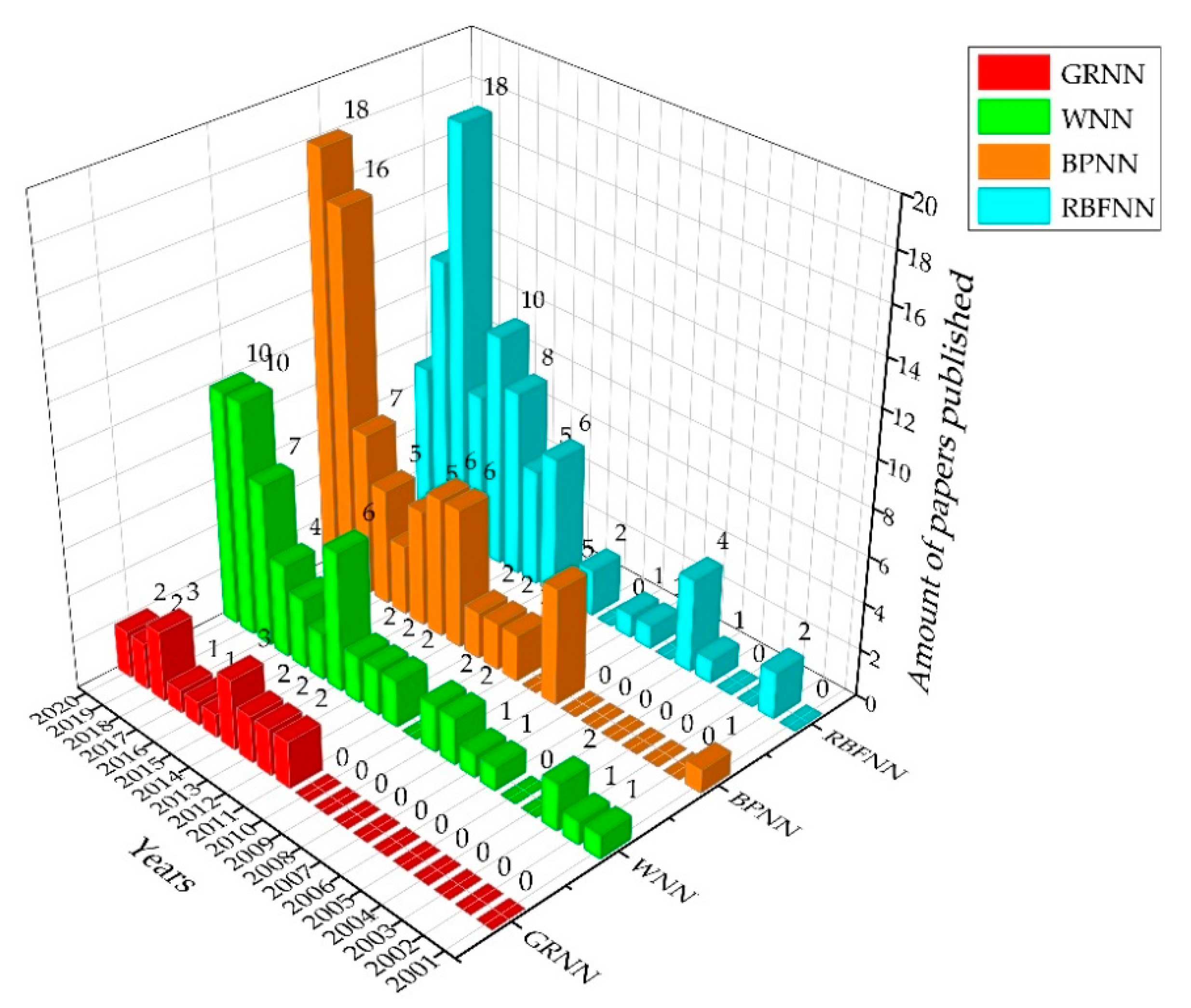
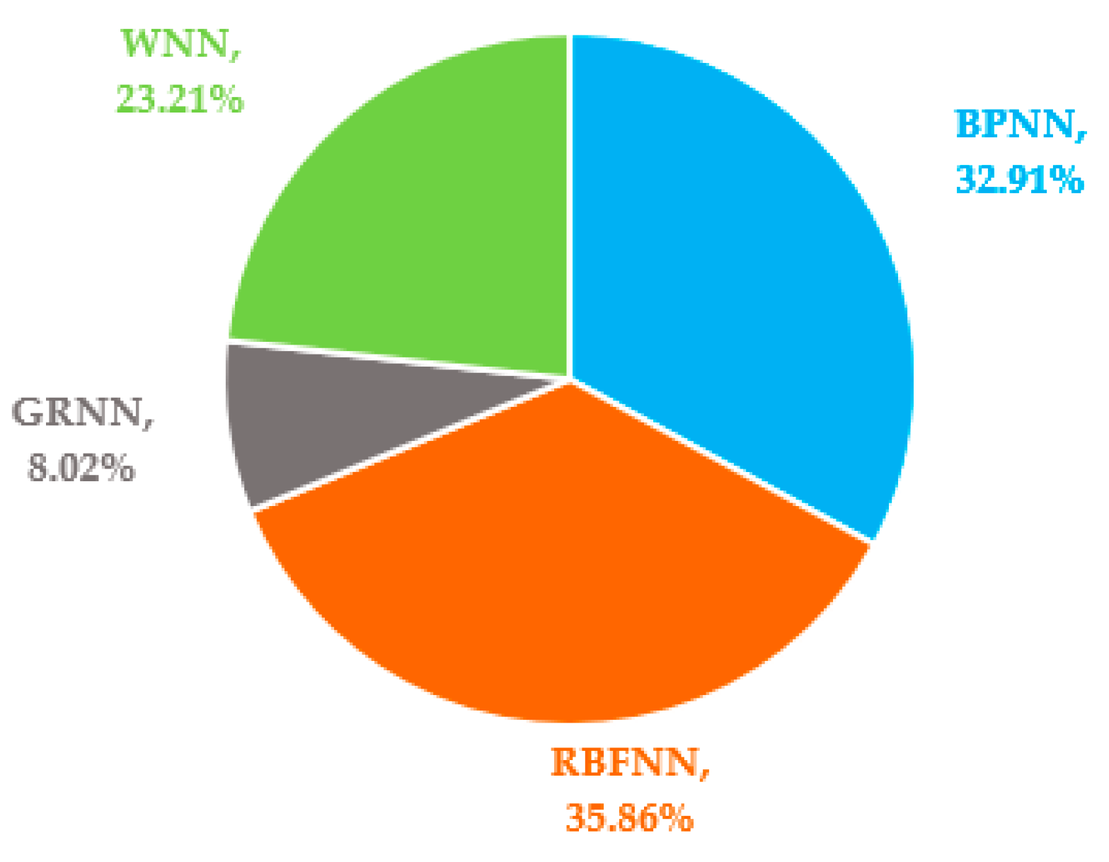
Use WoS to index the number of ANNs published in the oil and gas industry from 2001 to 2020 and the number of four different ANNs published in the oil and gas industry. The index results show that the publication volume of the four types of ANNs in the oil and gas industry is increasing, and the growth of WNN, BPNN and RBFNN is more significant;

(2)

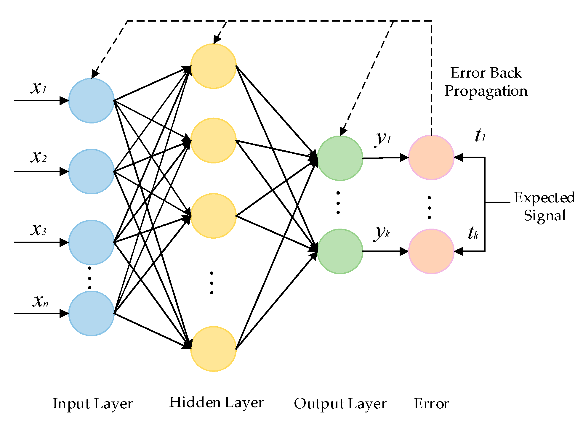
The network structure, hidden layer function, calculation process, and optimization algorithm of four kinds of ANNs are reviewed, and examples of the use of ANNs in the oil and gas industry and other industries are summarized and evaluated;

(3)

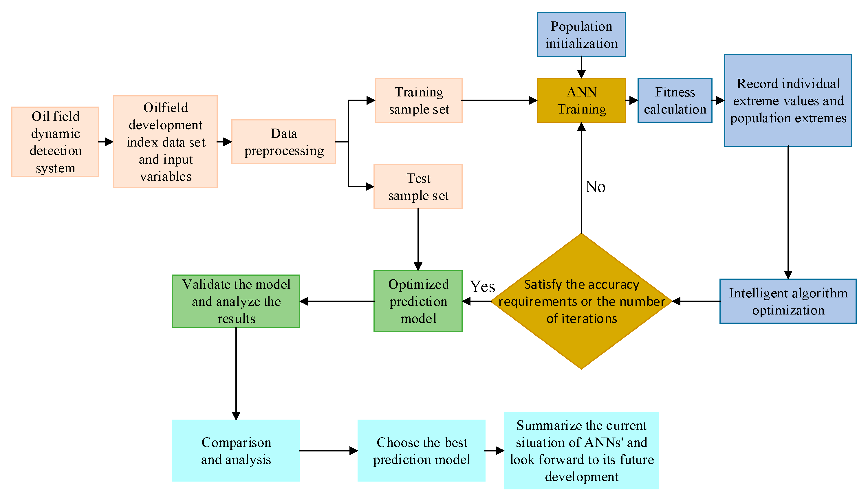
Establish a WOA-BPNN prediction model to verify the accuracy and effectiveness of ANNs prediction, and further verify the WOA-BPNN prediction model through the Arps output decline formula;

(4)

Through the method of combining theory and experiment, it will play a reference and guiding role for the future research of oil and gas field development index prediction;

(5)

The prediction model, when combined with the current status of actual oil and gas field development, helps point out the future development trends of ANNs in the oil and gas industry, in addition to others.

8.2. Future Areas of Research

The above summarizes the application of ANNs and an optimization algorithm combined with ANNs in oilfield development index prediction. This section will discuss the future research direction of ANNs in the petroleum industry and other industries.

Although various ANNs have achieved good results in solving the research and application of oilfield development index prediction, and their working principle is to approximate the nonlinear function as much as possible, they have not solved the problem of how multiple influencing factors interact to affect oilfield development index in theory. That is, they are only used as a mathematical tool for simple nonlinear analysis of many data. It does not involve the level of oil displacement mechanism. Only at the level of the oil displacement mechanism can we truly reflect the dynamic change law of oilfield development indicators and predict oilfield development indicators with the highest accuracy and efficiency. In the prediction of oilfield development indicators in the future, we can also try to combine ANN with oil displacement mechanisms to explain the interaction of various influencing factors on oilfield development indicators from the theoretical level.

Another future research direction is to establish a prediction system and model base [79,80,81] for an oilfield in a specific exploitation state, combining the experience of relevant oilfield development experts and the actual oilfield development. Using an intelligent discriminant analysis mechanism, selecting the best prediction model from numerous prediction methods and models that can predict the oilfield development index with high precision has become a hot issue in oilfield development in the future.

Although deep learning has attracted extensive attention in the oil field and other fields, there are still some problems to be solved in future research:

• For the problem of big data mining in the oilfield development index prediction model, it is necessary to extract the dynamic characteristics and knowledge reflecting oilfield development by using the deep learning convolutional neural network and the cyclic neural network;
• For the prediction methods and models of complex dynamic systems, the core components of intelligent prediction of oilfield development indicators, such as model base, method base and knowledge base, need to be solved theoretically and technically;
• With the improvement of digital oilfield construction levels, it is necessary to solve the problem of “reservoir-engineering-management” integrated artificial intelligence technology driven by big data cloud computing;
• New artificial neural networks and deep learning algorithms can be explored. Artificial neural networks and deep learning algorithms with good application effects in other fields can be transferred to the petroleum industry, and the research results of artificial neural networks and deep learning algorithms in the petroleum industry can also be transferred and applied to other fields.

With the development of artificial neural networks and deep learning algorithms, the biggest problem is the lack of data and information sharing among researchers. This information concerning model selection, variable selection, data processing, and verification are very important for the development of related fields. Therefore, the sharing of artificial neural networks and deep learning algorithms in the future also needs to be highly valued.

References

1. Zhong, Y.; Wang, S.; Luo, L. Mining knowledge of oilfield development index prediction model with deep learning. J. Southwest Pet. Univ. 2020, 42, 63–74. [Google Scholar]
2. Wenchao, F.; Hanqiao, J.; Junjian, L. Method for predicting late stage indicators of oilfield development based on uncertainty research. Pet. Geol. Recovery Effic. 2015, 22, 94–98. [Google Scholar]
3. Tao, W. Application of artificial neural network in recovery prediction of CO2 flooding. Spec. Oil Gas. Reserv. 2011, 18, 77–79. [Google Scholar]
4. Tao, W.; Yuedong, Y.; Liming, Z. Box—Behnken Study on Influencing Factors of carbon dioxide oil displacement effect by method. Fault Block Oil Gas Field 2010, 17, 15. [Google Scholar]
5. Qingjun, Y.; Chuncheng, D.; Yongli, Y. Application of artificial neural network in identification of low resistivity reservoirs. Spec. Oil Gas Reserv. 2001, 2, 8–10. [Google Scholar]
6. Chen, X.; Yan, Q. A Prediction Method of Crude Oil Output Based on Artificial Neural Network. In Proceedings of the 2011 International Conference on Computational and Information Sciences, Chengdu, China, 21–23 October 2011. [Google Scholar]
7. Nguyen, H.; Chan, C.; Wilson, M. Prediction of oil well production using multi-neural networks. In Proceedings of the Canadian Conference on Electrical and Computer Engineering, Winning, MB, Canada, 12–15 May 2002. [Google Scholar]
8. Khamehchi, E.; Abdolhosseini, H.; Abbaspour, R. Prediction of Maximum Oil Production by Gas Lift in an Iranian Field Using Auto-Designed Neural Network. Int. J. Pet. Geosci. Eng. 2014, 2, 138–150. [Google Scholar]
9. Kazerani, M.; Davoudian, A.; Zayeri, F. Assessing abstracts of Iranian systematic reviews and meta-analysis indexed in WOS and Scopus using PRISMA. Med. J. Islamic Repub. Iran 2017, 31, 104–109. [Google Scholar] [CrossRef] [PubMed]
10. Run Ge, J.; Zmeureanu, R. Forecasting Energy Use in Buildings Using Artificial Neural Networks: A Review. Energies 2019, 12, 3254. [Google Scholar] [CrossRef] [Green Version]
11. Ps, A.; Rdb, A.; Sks, B. Artificial Neural Networks in the domain of reservoir characterization: A review from shallow to deep models. Comput. Geosci. 2020, 135, 104357. [Google Scholar] [CrossRef]
12. Ghoddusi, H.; Creamer, G.; Rafizadeh, N. Machine learning in energy economics and finance: A review. Energy Econ. 2019, 81, 709–729. [Google Scholar] [CrossRef]
13. Saeed, R.; Ali, G.; Jassem, A.; Hoda, D.; Afshin, T. Prediction of Critical Multiphase Flow Through Chokes by Using A Rigorous Artificial Neural Network Method. Flow Meas. Instrum. 2019, 69, 101579. [Google Scholar] [CrossRef]
14. Wenhui, W.; Zhengshan, L.; Xinsheng, Z. Prediction of corrosion residual life of buried pipeline based on PSO-GRNN model. Surf. Technol. 2019, 48, 267–275. [Google Scholar]
15. Liang, H.; Wei, Q.; Lu, D. Application of GA-BP neural network algorithm in killing well control system. Neural Comput. Appl. 2021, 33, 949–960. [Google Scholar] [CrossRef]
16. Liu, Y.; Xie, S.; Zheng, L. Air-soil diffusive exchange of PAHs in an urban park of Shanghai based on polyethylene passive sampling: Vertical distribution, vegetation influence and diffusive flux. Sci. Total Environ. 2019, 689, 734–742. [Google Scholar] [CrossRef] [Green Version]
17. Li, R.; Zhang, H. BP neural network and improved differential evolution for transient electromagnetic inversion. Comput. Geosci. 2020, 137. [Google Scholar] [CrossRef]
18. Li, J.; Liang, G. Petrochemical equipment corrosion prediction based on BP artificial neural network. In Proceedings of the 2015 IEEE International Conference on Mechatronics and Automation, Beijing, China, 2–5 August 2015. [Google Scholar]
19. Dukui, Z.; Chenzhang, H.; Yuehua, P. Research Progress on prediction of CO2 corrosion rate of oil pipeline based on artificial neural network. Hot Work. Process 2021, 23, 25–31. [Google Scholar]
20. Rongbing, W.; Hongyan, X.; Bo, L.; Yong, F. Research on determination method of hidden layer node number of BP neu-ral network. Comput. Technol. Dev. 2018, 28, 31–35. [Google Scholar]
21. Ee, K.; Bin, I.; Bin, J. Adaptive Multilayered particle swarm optimized neural network (AMPSONN) for pipeline corrosion pre-diction. Int. J. Adv. Comput. Sci. Appl. 2017, 8, 499–508. [Google Scholar]
22. Supriyatman, D.; Sumarni, S.; Sidarto, K.A.; Suratman, R. Artificial neural networks for corrosion rate prediction in gas pipelines. In Proceedings of the SPE Asia Pacific Oil and gas Conference and Exhibition, Perth, Australia, 22–24 October 2012. [Google Scholar]
23. Linmao, M.; Defu, L.; Haixiang, G. Application of BP neural network based on genetic algorithm optimization in crude oil production prediction: Taking bed test area of Daqing Oilfield as an example. Math. Pract. Underst. 2015, 45, 117–128. [Google Scholar]
24. Trasatti, S. The contribution of neural networks to solve corrosion related problems. Adv. Mater. Res. 2010, 95, 23–27. [Google Scholar] [CrossRef]
25. Shaowei, P.; Hongjun, L. Study on dynamic prediction of oil saturation by GA-BP neural network. Comput. Technol. Dev. 2012, 12, 157–160. [Google Scholar]
26. Ren, C.Y.; Qiao, W.; Tian, X. Natural gas pipeline corrosion rate prediction model based on BP Neural network. Adv. Intell. Soft Comput. 2012, 147, 449–455. [Google Scholar]
27. Lei, S.; Bi, Y.; Lu, G. Application of BP Neural Network in Oil Field Production Prediction. In Proceedings of the 2010 Second World Congress on Software Engineering, Wuhan, China, 19–20 December 2010. [Google Scholar]
28. Yapeng, T.; Binshan, J. Prediction model of shale gas production decline based on Improved BP neural network based on genetic algorithm. Chin. Sci. Paper 2016, 11, 1710–1715. [Google Scholar]
29. Srinivas, M.; Patnailk, L.M. Adaptive probabilities of crossover and mutation in genetic algorithms. IEEE Trans. Syst. Man Cybern. 1994, 24, 656–667. [Google Scholar] [CrossRef] [Green Version]
30. Chongyu, S.; Yuduo, W. Optimization of BP neural network based on improved adaptive genetic algorithm. Ind. Control. Comput. 2019, 32, 67–69. [Google Scholar]
31. Qiyi, Q.; Chengxiang, G.; Shuai, W. Research on BP neural network optimization method based on particle swarm optimization and cuckoo search. J. Guangxi Univ. 2020, 45, 898–905. [Google Scholar]
32. Yurong, W.; Rigen, W. Prediction of static corrosion properties of re Ni Cu alloy cast iron based on RBF neural network. Weapon Mater. Sci. Eng. 2014, 37, 66–68. [Google Scholar]
33. Qian, W.; Maojin, T.; Yujiang, S. Prediction of relative permeability and calculation of water cut of tight sand-stone reservoir by radial basis function neural network. Pet. Geophys. Explor. 2020, 55, 864–872. [Google Scholar]
34. Song, C.F.; Hou, Y.B.; Du, J.Y. The prediction of grounding grid corrosion rate using optimized RBF network. Appl. Mech. Mater. 2014, 596, 245–250. [Google Scholar] [CrossRef]
35. Tatar, A.; Shokrollahi, A.; Mesbah, M. Implementing radial basis function networks for modeling CO2-reservoir oil mini-mum miscibility pressure. J. Nat. Gas Sci. Eng. 2013, 15, 82–92. [Google Scholar] [CrossRef]
36. Shaohua, X.; Congcong, B.; Yu, Z. Prediction of oilfield development index based on radial basis function process neural network. Calc. Technol. Autom. 2015, 34, 52–54. [Google Scholar]
37. Hong, L.; Wu, G.; Wang, T. Optimizing fracturing design with a RBF neural network based on immune principles. In Proceedings of the 2012 IEEE 11th International Conference on Cognitive Informatics and Cognitive Computing, Kyoto, Japan, 22–24 August 2012; IEEE: New York, NY, USA, 2012; pp. 336–340. [Google Scholar]
38. Shao, W.; Chen, S.; Cheng, Y.; Mahmpud, E.; Hursan, G. Improved RBF-Based NMR Pore-Throat Size, Pore Typing, and Permeability Models for Middle East Carbonates. In Proceedings of the SPE Annual Technical Conference and Exhibition, Dubai, The United Arab Emirates, 26–28 September 2016. [Google Scholar]
39. Xie, T.; Yu, H.; Hewlett, J.; Rozycki, P.; Wilamowski, B. Fast and efficient second-order method for training radial basis function networks. IEEE Trans. Neural Netw. Learn. Syst. 2012, 23, 609–619. [Google Scholar] [CrossRef]
40. Zhang, Z.; Yu, D. Comparison and research of BP and RBF neural networks in function approximation. Ind. Control. Comput. 2018, 31, 119–120. [Google Scholar]
41. Pi, J.; Ma, S.; Qiqi, Z. GRNN aeroengine exhaust temperature prediction model based on improved Drosophila algorithm optimization. J. Aeronaut. Dyn. 2019, 34, 8–17. [Google Scholar]
42. Hui, C.; Zegen, H.; Yongping, W. Application of generalized regression neural network technology in rapid evalu-ation of new oil fields. J. Chongqing Inst. Sci. Technol. 2019, 21, 42–45. [Google Scholar]
43. Donghu, C.; Weiyao, Z.; Huayin, Z. Prediction of oil well water cut by generalized regression neural network. J. Chongqing Univ. Sci. Technol. 2012, 14, 97–101. [Google Scholar]
44. Hongbing, H.; Zhihong, X. Generalized Regression Neural Network Optimized by Genetic Algorithm for Solving Out-of-Sample Extension Problem in Supervised Manifold Learning. Neural Process. Lett. 2019, 50, 2567–2593. [Google Scholar]
45. Wentao, P. A new fruit fly optimization algorithm:taking the financial distress model as an example. Knowl. Based Syst. 2012, 26, 69–74. [Google Scholar]
46. Yong, L.; Xuan, W.; Huiting, Z. Research on the prediction problem of improved Drosophila optimization algorithm and generalized regression neural network. World Sci. Technol. Res. Dev. 2014, 36, 272–276. [Google Scholar]
47. Hua, D.; Zongcheng, W.; Yicheng, G. Multi-objective optimization of fiber laser cutting based on generalized regression neural network and non-dominated sorting genetic algorithm. Infrared Phys. Technol. 2020, 108, 2267–2271. [Google Scholar]
48. Yipeng, J.; Qingshang, L.; Quan, Y. Rock burst prediction based on particle swarm optimization and generalized regres-sion neural network. J. Rock Mech. Eng. 2013, 32, 343–348. [Google Scholar]
49. Qinghua, Z.; Albert, B. Wavelet networks. IEEE Trans Neural Netw. 1992, 3, 889–895. [Google Scholar]
50. Zhe, C.; Tianjin, F. Research Progress on the combination of wavelet analysis and neural network. J. Electron. Inf. 2000, 22, 496–504. [Google Scholar]
51. Rong, G.; Jun, W. Application of fuzzy wavelet neural network in operation risk assessment of FRP pipe in active oil field. J. Xi’an Univ. Technol. 2012, 32, 980–986. [Google Scholar]
52. Zhichao, L.; Wenwen, Z.; Yihua, Z. Application of wavelet neural network in oilfield production prediction. Daqing Pet. Geol. Dev. 2008, 27, 52–54. [Google Scholar]
53. Jianli, L.; Yihua, Z.; Daojie, L. Prediction method of oilfield development performance index based on wavelet neural network. Nat. Gas Explor. Dev. 2008, 62, 66–87. [Google Scholar]
54. Ziqi, L.; Zhang, H. Research on oil price prediction based on sa-wnn model. Resour. Ind. 2020, 22, 58–64. [Google Scholar]
55. Youzhou, C.; Tao, R.; Peng, D. Tunnel settlement prediction based on artificial bee colony optimization wavelet neural nework. Mod. Tunn. Technol. 2019, 56, 56–61. [Google Scholar]
56. Junbao, Z.; Shanshan, R. Wavelet neural network short-term traffic flow prediction based on improved leapfrog algorithm. Softw. Guide 2020, 19, 50–54. [Google Scholar]
57. Xia, L.; Zongshang, L.; Yu, G.; Boyu, W. Analysis of main controlling factors of oil production based on machine learning. Inf. Syst. Eng. 2019, 94, 97–99. [Google Scholar]
58. Ruishu, F.; Wright, P.; Lu, J.; Devkota, F.; Lu, M.; Ziomek-Moroz, M.; Paul, R. Corrosion Sensors for Structural Health Monitoring of Oil and Natural Gas Infrastructure: A Review. Sensors 2019, 19, 3964–3995. [Google Scholar]
59. Renchang, Z.; Qian, L.; Lu, T. On-chip micro pressure sensor for microfluidic pressure monitoring. J. Micromech.Microengine. 2021, 31, 055013. [Google Scholar] [CrossRef]
60. Yang, C.; Liu, W.; Liu, N.; Su, J.; Li, L.; Xiong, L.; Long, F.; Zou, Z.; Gao, Y. Graphene Aerogel Broken to Fragments for a Piezoresistive Pressure Sensor with a Higher Sensitivity. ACS Appl. Mater. Interfaces 2019, 11, 33165–33172. [Google Scholar] [CrossRef]
61. Lei, G.; Xu, G.; Zhang, X.; Tian, B. Study on dynamic characteristics and compensation of wire rope tension based on oil pressure sensor. Adv. Mech. Eng. 2019, 11, 1–13. [Google Scholar]
62. Mengyao, Q.; Yi, Y.; Zeqing, L.; Zonglin, Y.; Xuebin, P. Contactless liquid level measurement system based on capacitive sensor. Sensor. Microsyst. 2021, 40, 81–84. [Google Scholar]
63. Xiaowei, F.; Yi, Z.; Peng, Y.; Jincheng, Z. Application of distributed optical fiber temperature monitoring technology in production and profile interpretation of fractured horizontal wells. Oil Gas Reserv. Eval. Dev. 2021, 11, 542–549. [Google Scholar]
64. Li, Z.; Wei, Z. Design and test of distributed optical fiber acoustic leakage monitoring system for gathering and transmission pipeline. Oil Gas Field Surf. Eng. 2021, 40, 57–64. [Google Scholar]
65. Xiufen, Q.; Feng, Z.; Zhiwei, S.; Qingsheng, J.; Ming, L.; Cong, S.; Changbang, H. Joint detection method of pipe-line damage based on distributed optical fiber sensing technology. Oil Gas Storage Transp. 2021, 40, 888–894. [Google Scholar]
66. Hongyuan, S.; Liang, M.; Yanan, Z.; Bing, C.; Shirui, Z.; Haifeng, Z. Research on real-time measurement technology of oilfield multiphase flow based on multi-sensor and SVR algorithm. Instrum. Users 2019, 26, 15–19. [Google Scholar]
67. Amin, A.; Mojtaba, A.; Fatemeh, A. Thermodynamic analysis PVT equation of state definition and gas injection review along with case study in three wells of Iranian oil field. Energy Sources Part A Recovery Util. Environ. Eff. 2020, 42, 1–19. [Google Scholar]
68. Tsekos, C.; Tandurella, S.; de Jong, W. Estimation of lignocellulosic biomass pyrolysis product yields using artificial neural networks. J. Anal. Appl. Pyrolysis 2021, 157, 105180. [Google Scholar] [CrossRef]
69. Alarifi, I.; Nguyen, M.; Hoang, M.; Naderi, B.; Ali, A. Feasibility of ANFIS-PSO and ANFIS-GA Models in Predicting Thermophysical Properties of Al2O3-MWCNT/Oil Hybrid Nanofluid. Materials 2019, 12, 3628. [Google Scholar] [CrossRef] [PubMed] [Green Version]
70. Marta, M.; Gregorio, F.; Valverde, A.; Krzemien, K.; Wodarski, P.; Riesgo, F. Optimizing Predictor Variables in Artificial Neural Networks When Forecasting Raw Material Prices for Energy Production. Energies 2020, 13, 2017–2031. [Google Scholar]
71. Nan, W.; Changjun, L.; Xiaolong, P.; Fanhua, Z.; Xinqian, L. Conventional models and artificial intelligence-based models for energy consumption forecasting: A review. J. Pet. Sci. Eng. 2019, 181, 106187. [Google Scholar] [CrossRef]
72. Liu, C.; Yue, C. A novel bionic swarm intelligent optimization algorithm: Firefly algorithm. Comput. Appl. Res. 2011, 28, 3295–3297. [Google Scholar]
73. Ramahlapane Lerato, M.R.; Mthulisi, V. A Model to Improve the Effectiveness and Energy Consumption to Address the Routing Problem for Cognitive Radio Ad Hoc Networks by Utilizing an Optimized Cuckoo Search Algorithm. Energies 2021, 14, 3464–3477. [Google Scholar]
74. Shaofeng, L.; Sheng, L. A review of cuckoo search algorithm. Comput. Eng. Des. 2015, 36, 1063–1067. [Google Scholar]
75. Takagi, T.; Sugeno, M. Fuzzy identification of systems and its applications to modeling and control. IEEE Trans. Syst. Man Cybern. 1985, 15, 116–132. [Google Scholar] [CrossRef]
76. Glowacz, A. Fault diagnosis of electric impact drills using thermal imaging. Measurement 2021, 171, 108815. [Google Scholar] [CrossRef]
77. Muhammad, Z.; Muhammad, K.; Khan, F. Application of ANFIS, ANN and fuzzy time series models to CO2 emis-sion from the energy sector and global temperature increase. Int. J. Clim. Chang. Strateg. Manag. 2019, 11, 622–642. [Google Scholar]
78. Wang, D.; Peng, J.; Yu, Q.; Chen, Y.; Yu, H. Support Vector Machine Algorithm for Automatically Identifying Depositional Microfacies Using Well Logs. Sustainability 2019, 11, 1919. [Google Scholar] [CrossRef] [Green Version]
79. Sun, X.; Zhang, X. Research on the application of data mining technology in Oilfield informatization construction. China Manag. Informatiz. 2021, 24, 124–125. [Google Scholar]
80. Wang, R. Data mining technology and application in the era of big data. Light Ind. Sci. Technol. 2021, 37, 72–73. [Google Scholar]
81. Liang, Y.; Huang, K.; Wei, T.; Li, R. Research on network security and prediction technology in the era of big data. Comput. Meas. Control 2021, 29, 168–171. [Google Scholar]
Figure 1. Annual publication volume of ANNs in the field of oil and gas.
Energies 14 05844 g001
Figure 2. Annual publication volume of 4 kinds of ANNs in the oil and gas field.
Energies 14 05844 g002
Figure 3. Percentage of 4 different ANNs’ publications in the oil and gas industry (2001–2020).
Energies 14 05844 g003
Figure 4. Research block diagram of oilfield development index prediction.
Energies 14 05844 g004
Figure 5. Schematic diagram of BPNN structure.
Energies 14 05844 g005
Figure 6. Logsig function curve.
Energies 14 05844 g006
Figure 7. Tansig function curve.
Energies 14 05844 g007
Figure 8. Schematic diagram of RBFNN structure.
Energies 14 05844 g008
Figure 9. Curves of three typical radial basis functions.
Energies 14 05844 g009
Figure 10. Schematic diagram of GRNN structure.
Energies 14 05844 g010
Figure 11. Schematic diagram of WNN structure.
Energies 14 05844 g011
Figure 12. Morlet wavelet basis function curve.
Energies 14 05844 g012
Figure 13. Prediction model of oilfield development index based on ANN.
Energies 14 05844 g013
Figure 14. Comparison results between: (a) BPNN training value and actual data. (b) WOA-BPNN training value and actual data.
Energies 14 05844 g014
Figure 15. Comparison of actual value, BPNN predicted value andWOA-BPNN predicted value.
Energies 14 05844 g015
Figure 16. Comparison of relative error between: (a) BPNN training value and WOA-BPNN training value. (b) BPNN predicted value and WOA-BPNN predicted value.
Energies 14 05844 g016
Figure 17. Regression analysis of: (a) BPNN training set, prediction set and actual data. (b) WOA-BPNN training set, prediction set and actual data.
Energies 14 05844 g017