Steady-State Stand-Alone Power Flow Solvers for Integrated Transmission-Distribution Networks: A Comparison Study and Numerical Assessment

Abstract

This paper compares and assesses several numerical methods that solve the steady-state power flow problem on integrated transmission-distribution networks. The integrated network model consists of a balanced transmission and an unbalanced distribution network. It is important to analyze these integrated electrical power systems due to the changes related to the energy transition. We classified the existing integration methods as unified and splitting methods. These methods can be applied to homogeneous (complete three-phase) and hybrid (single-phase/three-phase) network models, which results in four approaches in total. These approaches were compared on their accuracy and numerical performance—CPU time and number of iterations—to demonstrate their applicability on large-scale electricity networks. Furthermore, their sensitivity towards the amount of distributed generation and the addition of multiple distribution feeders was investigated. The methods were assessed by running power flow simulations using the Newton–Raphson method on several integrated power systems up to 25,000 unknowns. The assessment showed that unified methods applied to hybrid networks performed the best on these test cases. The splitting methods are advantageous when complete network data sharing between system operators is not allowed. The use of high-performance techniques for larger test cases containing multiple distribution networks will make the difference in speed less significant.

1. Introduction

The study of steady-state power flow solvers for integrated electricity networks is gaining more attention due to challenges that arise from the energy transition. Integrated electricity networks are networks that consist of a transmission and a distribution network. Due to the energy transition, more renewable energy is entering the grid at the distribution level, and demand-side participation as a mechanism to balance frequency is increasing, even as the electricity consumption increases due to the rise of, amongst others, electric vehicles [1,2]. Integrated network models are key to study the interaction that these networks have with each other in this changing environment. On top of that, these challenges increase the size of the network and the frequency of network state analysis. Therefore, load flow solvers should not only be capable of solving the integrated power flow problem, but also run these computations fast and efficiently.

Steady-state load flow analysis is an important tool used for grid operation and planning. Much attention has been paid so far to efficient solvers for the load flow analysis of separate networks [3,4]. In these separate network models, transmission networks include the total load of the distribution network as a balanced load bus, while distribution networks include the transmission network as the slack bus. Although developments of these separate network solvers continue, the focus in this work is on methods that can solve the power flow problem on integrated transmission-distribution network models efficiently. The research fields that are investigating these integrated power systems can be divided into two categories: stand-alone methods [5,6] and cosimulation methods [7,8]. Although cosimulation is an important field and valuable for system operators—because many operators use their own software tools for operation and planning—the focus of this work is on stand-alone methods. The eventual goal of this study is to obtain fast load flow solvers, and more numerical efficiency is expected from stand-alone methods.

Although legislation sometimes prohibits the use of stand-alone methods [6], enough potential use cases for these methods exist, to name a few: Some countries run their electricity network by one system authority being responsible for both transmission and distribution network operation, such as in Brazil [9]. Next to that, cooperation at the international level between system operators is increasing, such as in the European Union by ENTSO-E [10], which allows the use of a stand-alone tool for complete operation and planning. On top of that, one may argue that the innovations that arise from stand-alone methods may not only be valuable for the integrated system field, but also for merely balanced systems where imbalance arises on only a few lines [9].

Integrating transmission and distribution network models are a challenging task, firstly because the transmission network is a balanced network and therefore modeled using a single phase only, while the distribution network is in general not balanced and thus modeled using three phases [11]. Furthermore, also transmission and distribution solvers have been developed separately because of the distinct properties of the networks. Transmission systems are often solved using the power mismatch formulation of Newton–Raphson or with fast decoupled load flow methods [3]. The solvers that have proven to be better for distribution systems are, to list a few, the Newton–Raphson method applied to the current mismatch formulation [12], forward backward sweep methods [13], or modified $Z_{bus}$ methods [14]. Nevertheless, power flow solvers for integrated network models are being developed, and the field that studies these methods is emerging [15].

A literature review showed that multiple stand-alone approaches exist that integrate transmission and distribution network models. We categorized them into unified [5] and master–slave splitting [6] methods. These approaches can be applied to homogeneous (complete three-phase) or hybrid (single-phase/three-phase) networks [5,16]. Unified methods, also called the MonoTri formulation by the authors [5], make a new integrated network of the two separate networks and solve them in one go. The master–slave-splitting-based distributed global power flow method—which will be called the master–slave splitting method during the rest of this work—adds an additional iterative scheme between the methods such that the networks can be solved separately. The complete system reaches convergence as soon as both the separate systems and the splitting method have converged.

Over the years, improvements of these methods have been made either in the field of dynamic analysis or to handle more physical details of the network itself. The authors of the MonoTri formulation introduced this concept in 2008 and recently published new work in which the MonoTri formulation was used for transient stability analysis [9]. The authors of the splitting formulation introduced this concept in 2005 [17] and have been working on improvements since then [6,18,19], in which the latest work gave a clear description of the master–slave splitting methods including an extensive convergence analysis and improvements that have been made when loops and distributed generation are considered [6].

Additional improvements have been made. In [16], the splitting methods were applied and compared to steady-state unbalanced test cases. In [20], they were tested for dynamic analysis of unbalanced test cases. The work of [21] improved the speed of the MSS methods when radial distribution networks are heavily loaded. They did so by using Thevenin equivalents as the input for the distribution network, instead of taking the voltage of the connecting bus of the transmission network as the input. As defined in [21], the Thevenin equivalent is a type of single-port equivalent, which replaces an entire network by an equivalent circuit consisting of a single voltage in series with an impedance. This means that the impact of the transmission network on the distribution network can be studied by only considering the Thevenin equivalents. In order to calculate the equivalents, a phasor measurement unit (PMU) needs to be installed along the network in order to determine the (voltage, current) pairs at the interface of the two subsystems.

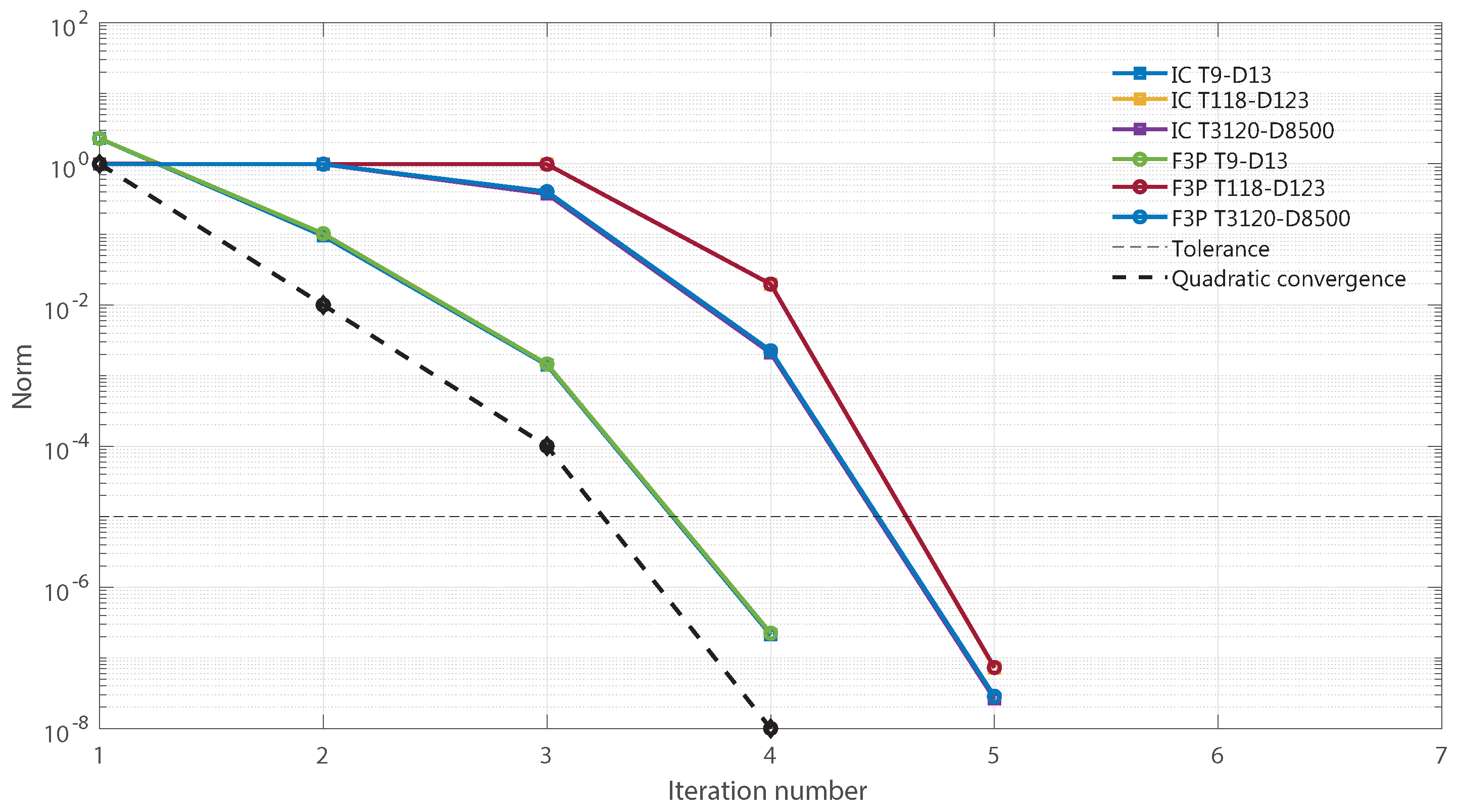
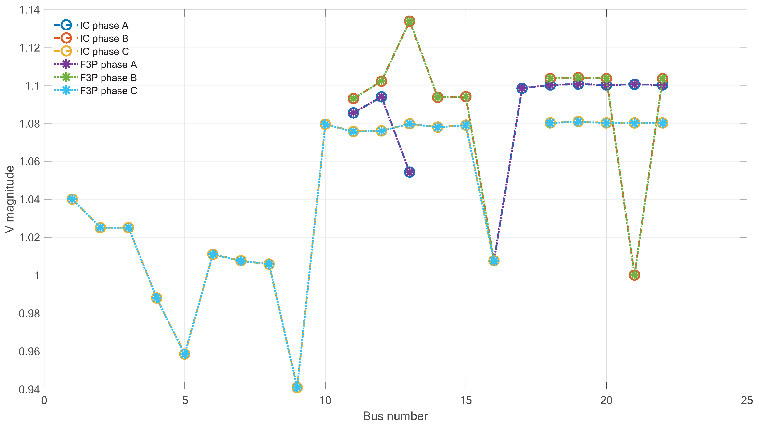
So far, the stand-alone integration methods have been developed, improved, and validated, but what lacks is a thorough and independent comparison study of both methods under the same circumstances. This work consists of a review of the existing stand-alone methods and an assessment of these methods by implementing them on the same set of integrated test cases. The same category of solvers, which are different versions of the Newton–Raphson solver with a direct $LU$-factorization, is adopted to diminish external influences in order to obtain an objective comparison.

The review in this work included a generic description of both methods and a list of the advantages and disadvantages related to their numerical performance, physical details, and usability. The numerical assessment included an assessment of the steady-state load flow performance of the methods and their sensitivity towards the physical conditions of the network such as the addition of multiple distribution feeders and the amount of distributed generation. The conditions on which the methods were assessed are: the convergence rate, CPU time, and robustness. To do so, integrated networks were created from standard IEEE transmission and distribution test networks. The largest integrated network contained around 25,000 unknowns. The end of the paper contains a discussion about which of the methods can be scaled efficiently to large and realistic networks, in order to fulfill the requirements of the prospected transforming electricity grids.

This paper is organized as follows. Section 2 contains a generic representation of separate electricity transmission and distribution networks, their distinct characteristics, and the (adapted) Newton–Raphson method as a fast and robust solver. Section 3 includes a uniform description of the different integration methods and integrated network models and an extensive review of the methods including a list of the advantages and disadvantages. Section 4 consists of the objective assessment of the numerical performance of the methods by applying them on the same set test cases. Section 5 gives insight into their applicability to realistic and large networks including the main distinctions and comparisons between the methods that arise. Section 6 contains concluding remarks and suggestions for future work.

2. The Power Flow Problem in Single-Phase and Three-Phase Representation

An electricity network model is represented as a graph consisting of buses $i=1,...,N$, representing generators, loads, and shunts and branches representing transformers and cables. The steady-state power flow problem of a network determines the voltages $V_i$ of each bus given the power supply and demand $S_i$ of each bus and the admittance $Y_{ij}$ of each branch [3]. The transmission network, which is a balanced network, is modeled as a single-phase network, where a represents the phase (Appendix A):

$$\begin{array}{c}\hfill S_i^a=V_i^a{\overline{I}}_i^a=V_i^a{\left(\overline{Y\mathbf{V}}\right)}_i^a=V_i^a\sum _{j=1}^N{\overline{Y}}_{ij}^a{\overline{V}}_j^a\end{array}$$

(1)

Complex power consists of an active (real) and reactive (imaginary) part: $S=P+\iota Q$. The power flow problem is solved using the Newton–Raphson solver applied to the power mismatch formulation (NR-P) to compute the unknown quantities at each bus i. The power mismatch formulation is written as: $\Delta S_i=S_{s,i}-V_i{\sum }_{j=1}^N{\overline{Y}}_{ij}{\overline{V}}_j\approx 0$ [3]. Assembling this equation for every bus in the network in an active and reactive component yields the following power mismatch vector:

$$\mathbf{F}\left(\mathbf{x}\right)=\left[\begin{array}{c}\Delta P\\ \Delta Q\end{array}\right]=\left[\begin{array}{c}{P}_s-P\left(\mathbf{x}\right)\\ Q_s-Q\left(\mathbf{x}\right)\end{array}\right]=0,$$

(2)

where $\mathbf{x}$ represents the state variables $x_i={\left[\begin{array}{cc}{\delta }_i& |V_i|\end{array}\right]}^T$, which form the voltage in the phasor notation $V_i=\left|V\right|exp{\left(\iota \delta \right)}_i$.

Distribution systems are unbalanced; therefore, the distribution network is modeled using all three phases $a,b,$ and c [22]. The power flow Equation (1) in three phases is described by:

$$S_i^p=V_i^p\overline{I_i^p}=V_i^p\sum _{j=1}^N\sum _{q=a,b,c}\overline{Y_{ij}^{pq}}\overline{V_j^q},p\in \{a,b,c\}.$$

(3)

The Newton–Raphson three-phase current injection method (TCIM) [12] is used to solve the distribution networks. Instead of applying the standard Newton–Raphson method to power mismatches, Ohm’s law is directly used, resulting in the following current mismatch vector:

$$\begin{array}{c}\hfill \mathbf{F}\left(\mathbf{x}\right)=\left[\begin{array}{c}\Delta {\mathbf{I}}^{Re,abc}\left(\mathbf{x}\right)\\ \Delta {\mathbf{I}}^{Im,abc}\left(\mathbf{x}\right)\end{array}\right]=\left[\begin{array}{c}{\mathbf{I}}_s^{Re,abc}-{\mathbf{I}}^{Re,abc}\left(\mathbf{x}\right)\\ {\mathbf{I}}_s^{Im,abc}-{\mathbf{I}}^{Im,abc}\left(\mathbf{x}\right)\end{array}\right].\end{array}$$

(4)

Loads, shunt, transformers, and regulators can be modeled in several configurations. Details can be found in the full version of this work [23].

3. Integration Methods

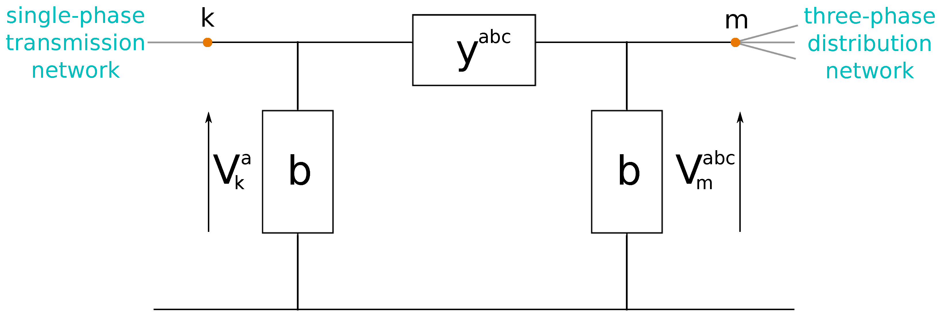
The transmission and distribution networks are connected to each other via a substation. The substation is a series of tap-changing transformers that transform high-voltage to low-voltage power. This substation can be modeled as a $\pi$-element that connects the transmission network from the left and the distribution network from the right, as seen in Figure 1. The single-phase/three-phase connection results in a dimension mismatch at this substation.

Table 1. Representation of the parameters in transmission and distribution network models.

Parameter	Transmission	Distribution
$S_i$	${\left[S^a\right]}_i$	${\left[S^a{S}^b{S}^c\right]}_i^T$
$V_i$	${\left[V^a\right]}_i$	${\left[V^a{V}^b{V}^c\right]}_i^T$
$Y_{ij}$	${\left[\begin{array}{cc}\underset{1\times 1}{Y_{11}^a}& \underset{1\times 1}{Y_{12}^a}\\ \underset{1\times 1}{Y_{21}^a}& \underset{1\times 1}{Y_{22}^a}\end{array}\right]}_{ij}$	${\left[\begin{array}{cc}\underset{3\times 3}{Y_{11}^{abc}}& \underset{3\times 3}{Y_{12}^{abc}}\\ \underset{3\times 3}{Y_{21}^{abc}}& \underset{3\times 3}{Y_{22}^{abc}}\end{array}\right]}_{ij}$

shows the single-phase and three-phase representation of S, V, and Y in the network models.

We classified the approaches to run stand-alone computations on integrated networks as unified and splitting methods and the two ways of modeling integrated networks as homogeneous and as hybrid networks. The unified method solves the integrated system as a whole [5]: The transmission network, substation, and distribution network are connected as one integrated network and then solved. The splitting method iterates between the two networks, and at each iteration, it solves the networks separately [6]. In the splitting method, the substation is part of the distribution network model. This method is similar to the cosimulation approach where the separate domains are solved on its own and coupled using an iterative scheme [7].

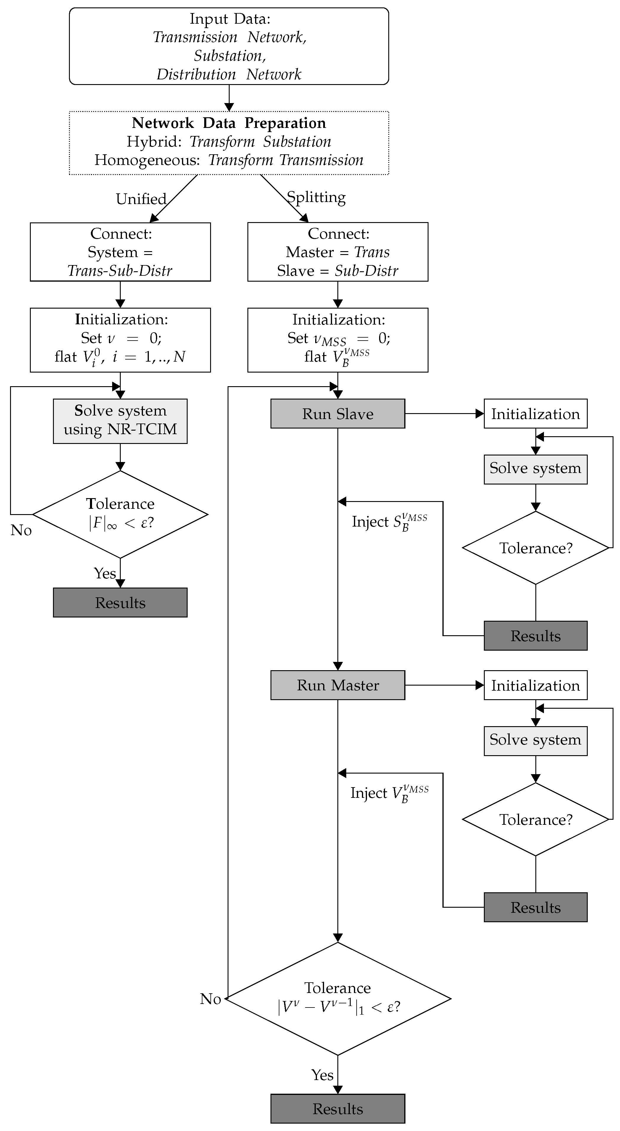
Homogeneous networks are networks where both the transmission and distribution network are modeled in three phases. It requires a transformation of the transmission network. Hybrid networks keep the transmission network as a single-phase model, but require a transformation of the substation model. We call the unified approach applied to homogeneous networks the (F3P) method and that applied to hybrid networks the interconnected (IC) method. We call all splitting methods master–slave splitting (MSS) methods. We define the MSS methods based on the network model they are applied to, e.g.,: the splitting approach applied to hybrid networks is called the MSS-hybrid method.

Table 2. Classification of numerical methods to solve integrated systems.

	Integrated Approach
Network Model	Unified	Splitting
Hybrid	Interconnected (IC) Transform substation Solve as a whole	MSS-hybrid Transform substation Extra iterative scheme
Homogeneous	Full three-phase (F3P) Transform Transmission Solve as a whole	MSS-homo Transform Transmission Extra iterative scheme

gives an overview of the methods.

3.1. Unified Methods

Unified methods solve the integrated system using one iterative scheme applied to the entire integrated network. The substation is modeled as a transformer that connects the two networks. It connects a load bus of the transmission network and the original slack bus of the distribution network, which then changes to a load bus. The entire system is solved using one algorithm.

3.1.1. The Full Three-Phase Method

The full three-phase method (F3P) is the unified method applied to homogeneous networks. Unbalanced distribution networks are modeled in three phases; the transmission networks requires a transformation. This transformation is based on the assumption that the transmission system is balanced: the phases b and c can be deducted from the first phase a, and the voltage $V^a$, the complex power $S^a$, and the admittance $Y_a$ of all the transmission buses $i=1,...,N$ are transformed to their three-phase equivalents. The following transformer matrices are used:

$$\begin{array}{c}\hfill {\mathbf{T}}_{\mathbf{1}}={\left[\begin{array}{ccc}1& a^2& a\end{array}\right]}^{T}and{\mathbf{T}}_{\mathbf{2}}={\left[\begin{array}{ccc}1& 1& 1\end{array}\right]}^T,a=e^{\frac{2}{3}\pi \iota },\end{array}$$

and identity matrix ${\mathbf{I}}_{3\times 3}$. This results in the following:

$$\begin{array}{cc}\hfill {\mathbf{T}}_{\mathbf{1}}{\left[V^a\right]}_i& ={\left[\begin{array}{ccc}{V}^a& V^b& V^c\end{array}\right]}_i^T,\hfill \end{array}$$

(5)

$$\begin{array}{cc}\hfill {\mathbf{T}}_{\mathbf{2}}{\left[\begin{array}{c}{S}^a\end{array}\right]}_i& ={\left[\begin{array}{ccc}{S}^a& S^b& S^c\end{array}\right]}_i^T,\hfill \end{array}$$

(6)

$$\begin{array}{ccc}& & \begin{array}{cc}3& 3\end{array}\\ {\left[\begin{array}{cc}{Y}_{11}^a\otimes {\mathbf{I}}_{3\times 3}& Y_{12}^a\otimes {\mathbf{I}}_{3\times 3}\\ Y_{21}^a\otimes {\mathbf{I}}_{3\times 3}& Y_{22}^a\otimes {\mathbf{I}}_{3\times 3}\end{array}\right]}_{ij}=& \begin{array}{c}3\\ 3\end{array}& {\left[\begin{array}{cc}{Y}_{11}^{abc}& Y_{12}^{abc}\\ Y_{21}^{abc}& Y_{22}^{abc}\end{array}\right]}_{ij}\end{array}.$$

(7)

3.1.2. The Interconnected Method

The interconnected method (IC) is the unified method applied to hybrid networks. The substation couples the single-phase quantities of bus k at the transmission side to the three-phase quantities at bus m at the distribution side. Therefore, it needs a transformation of its nodal admittance matrix $Y_{km}$ [5]. The $\pi$-element model of the connecting substation is depicted in Figure 1. The following four transformer matrices are used:

$${\mathbf{T}}_{\mathbf{1}},{\mathbf{T}}_{\mathbf{3}}=\frac{1}{3}\left[1a{a}^2\right],{\mathbf{T}}_{\mathbf{4}}=\frac{1}{3}\left[111\right],{\mathbf{T}}_{\mathbf{5}}=\frac{1}{3}\left[1a^{2}a\right],$$

where $a=e^{\frac{2}{3}\pi \iota }$, to establish the connection of bus k and m via the admittance matrix $Y_{km}$. This transformation is based on the assumption that the connecting bus k is perfectly balanced. This means that the single-phase and three-phase quantities are related as follows:

$$\begin{array}{}\mathrm{(8)}& \hfill {\left[\begin{array}{ccc}{V}^a& V^b& V^c\end{array}\right]}_k^T& =& {\mathbf{T}}_{\mathbf{1}}{\left[\begin{array}{c}{V}^a\end{array}\right]}_k,\hfill \mathrm{(9)}& \hfill {\left[\begin{array}{c}{I}^a\end{array}\right]}_k& =& {\mathbf{T}}_{\mathbf{3}}{\left[\begin{array}{ccc}{I}^a& I^b& I^c\end{array}\right]}_k^T,\hfill \mathrm{(10)}& \hfill {\left[\begin{array}{c}{S}^a\end{array}\right]}_k& =& {\mathbf{T}}_{\mathbf{4}}{\left[\begin{array}{ccc}{S}^a& S^b& S^c\end{array}\right]}_k^T.\hfill \end{array}$$

The change of the transformer substation depends on whether the unified system is solved using NR-Power or NR-TCIM.

Using Current Injections

The NR-TCIM method uses Ohm’s law directly. The relation between node k and m is expressed as follows [5]:

$$\begin{array}{c}\hfill I=YV\iff \left[\begin{array}{c}{I}_k\\ I_m\end{array}\right]=\left[\begin{array}{cc}{Y}_{11}& Y_{12}\\ Y_{21}& Y_{22}\end{array}\right]\left[\begin{array}{c}{V}_k\\ V_m\end{array}\right]\end{array}$$

(11)

If node k and m are both modeled in three phases, the following holds:

$$\begin{array}{cc}\hfill I_k^{abc}& =Y_{11}^{abc}{V}_k^{abc}+Y_{12}^{abc}{V}_m^{abc},\hfill \end{array}$$

(12)

$$\begin{array}{cc}\hfill I_m^{abc}& =Y_{21}^{abc}{V}_k^{abc}+Y_{22}^{abc}{V}_m^{abc}.\hfill \end{array}$$

(13)

Equation (12) is multiplied by ${\mathbf{T}}_{\mathbf{3}}$ to obtain $I_k^a$:

$$\begin{array}{cc}\hfill I_k^a={\mathbf{T}}_{\mathbf{3}}{\mathbf{I}}_k^{abc}& ={\mathbf{T}}_{\mathbf{3}}{Y}_{11}^{abc}{V}_k^{abc}+{\mathbf{T}}_{\mathbf{3}}{Y}_{12}^{abc}{\mathbf{V}}_m^{abc}.\hfill \end{array}$$

(14)

Accordingly, ${\mathbf{V}}_k^{abc}$ is substituted into Equations (13) and (14) by ${\mathbf{T}}_{\mathbf{1}}{V}_k^a$ (Equation (8)):

$$\begin{array}{cc}\hfill I_k^a={\mathbf{T}}_{\mathbf{3}}{\mathbf{I}}_k^{abc}& ={\mathbf{T}}_{\mathbf{3}}{Y}_{11}^{abc}{\mathbf{T}}_{\mathbf{1}}{V}_k^a+{\mathbf{T}}_{\mathbf{3}}{Y}_{12}^{abc}{\mathbf{V}}_m^{abc},\hfill \end{array}$$

(15)

$$\begin{array}{cc}\hfill {\mathbf{I}}_m^{abc}& =Y_{21}^{abc}{\mathbf{T}}_{\mathbf{1}}{V}_k^a+Y_{22}^{abc}{V}_m^{abc}.\hfill \end{array}$$

(16)

Equations (15) and (16) result in this new admittance matrix:

$$\begin{array}{ccc}& & \begin{array}{cc}1& 3\end{array}\\ Y_{km}=& \begin{array}{c}1\\ 3\end{array}& {\left[\begin{array}{cc}{\mathbf{T}}_{\mathbf{3}}\left[Y_{11}^{abc}\right]{\mathbf{T}}_{\mathbf{1}}& {\mathbf{T}}_{\mathbf{3}}\left[Y_{12}^{abc}\right]\\ \left[Y_{21}^{abc}\right]{\mathbf{T}}_{\mathbf{1}}& Y_{22}^{abc}\end{array}\right]}_{km}\end{array}$$

(17)

Using Power Injections

The deduction of the transformed admittance matrix $Y_{km}$ starting from the power equations, $S_i=V_i{\left(\overline{Y\mathbf{V}}\right)}_i$, is performed in a similar way [5]. The extended version of this work [23] contains a detailed description. The new nodal admittance matrix, deducted from power equations, is the following:

$$\begin{array}{ccc}& & \begin{array}{cc}1& 3\end{array}\\ Y_{km}=& \begin{array}{c}1\\ 3\end{array}& {\left[\begin{array}{cc}{\mathbf{T}}_{\mathbf{5}}\left[Y_{kk}^{abc}\right]{\mathbf{T}}_{\mathbf{1}}& {\mathbf{T}}_{\mathbf{5}}\left[Y_{km}^{abc}\right]\\ \left[Y_{mk}^{abc}\right]{\mathbf{T}}_{\mathbf{1}}& Y_{\mathit{mm}}^{abc}\end{array}\right]}_{km}\end{array}.$$

(18)

3.2. Master–Slave Splitting Methods

The splitting approach appoints the transmission network as the master and the distribution network as the slave [6]. In the splitting methods, the substation is part of the distribution network model. The methods can also be applied to homogeneous (MSS-homo) and hybrid (MSS-hybrid) networks. In contrast to the unified methods, the MSS methods keeps the master and the slave as two separate domains and introduces an extra iterative scheme between the domains, the MSS scheme. The two domains have one overlapping bus, and this bus is called the boundary bus [6]. The boundary bus is the bus connected to the left side of the substation model and acts as the slack bus for the slave. It can be any load bus of the transmission system.

3.2.1. Algorithmic Approach

The algorithmic approach of the MSS scheme goes as follows: (1) initialize the voltage $V^b$ of the boundary bus; (2) start with the slave by initializing the rest of the voltages, and then, solve this system; we obtain the complex power of the boundary bus, $S_B$, required as the initial input for the load bus of the master; (3) inject $S_B$ into the master; (4) initialize the rest of the master, and obtain an updated voltage of the boundary bus $V_B$; (5) compare $V_B$ with the voltage from the previous MSS iteration. If it is lower than the tolerance value ${\epsilon }_{MSS}={10}^{-5}$, the MSS system has converged. These steps are summarized in Algorithm 1.

Algorithm 1 The Master-Slave Splitting Iterative Scheme.

1: Set iteration counter $\nu =0$. Initialize the voltage $V_B^0$ of the distribution system.

2: Solve the distribution system. Output: $S_B^{\nu +1}$.

3: Inject $S_B^{\nu +1}$ into the transmission system.

4: Solve the transmission system. Output: $V_B^{\nu +1}$.

5: Is $|V_B^{\nu +1}-V_B^{\nu }{|}_1>{\epsilon }_{MSS}$? Repeat Steps 2 to 5.

As the MSS method solves the transmission and distribution systems separately, it allows for using different algorithms per domain. In this way, the distribution system is solved using the advantageous NR-TCIM method and the transmission system using the NR-power method. Furthermore, the MSS method can be applied to homogeneous networks and to hybrid networks [16], the first one requiring a transformation of the entire master domain, the latter requiring a transformation of the boundary bus only.

3.2.2. The MSS Homogeneous Method

The MSS method applied to homogeneous networks requires a transformation of the single-phase transmission system. The balanced transmission system is transformed in the same way as in the F3P method. The voltage, power, and admittance of all buses $i=1,\cdots ,N$ are transformed to three-phase equivalents. This idea is summarized in Equations (5)–(7) of Section 3.1.1.

3.2.3. The MSS-Hybrid Method

The MSS method applied to hybrid systems keeps the transmission system in a single phase. The original designers of the splitting method [6] transformed the complex power and the voltage of the boundary bus after one run of the slave and the master, respectively. First, the three-phase complex power $S_B$ is transformed into a single-phase quantity. Once the master system is solved, the voltage $V_{B}B$ is transformed to a three-phase quantity. Here, again, the transformation is based on the assumption that the boundary bus is completely balanced. Balanced three-phase power in pu is related to single-phase power in (10) according to the following relation:

$$\left[S^a\right]={\mathbf{T}}_{\mathbf{4}}{\left[\begin{array}{ccc}{S}^a& S^b& S^c\end{array}\right]}^T,$$

(19)

where ${\mathbf{T}}_{\mathbf{4}}=\frac{1}{3}\left[111\right],\mathrm{and}a=e^{\frac{2}{3}\pi \iota }$. The voltage of the boundary bus has the same relation as in (8):

$${\left[\begin{array}{ccc}{V}^a& V^b& V^c\end{array}\right]}_B^T={\mathbf{T}}_{\mathbf{1}}{\left[\begin{array}{c}{V}^a\end{array}\right]}_B,$$

(20)

where ${\mathbf{T}}_{\mathbf{1}}={\left[1a^{2}a\right]}^T,\mathrm{and}a=e^{\frac{2}{3}\pi \iota }$.

Algorithm 1 requires two extra lines: Transformation (19) is added after Step 2 and (20) after Step 4 of Algorithm 1. These steps are similar to transforming the nodal admittance matrix of the substation, which is connected to the slave, directly, in the same manner as explained in Section 3.1.2. In this way, the splitting approach no longer requires the addition of the two extra lines after Steps 2 and 4. Furthermore, it makes the description of the methods applied to hybrid networks generic.

The MSS methods reach convergence if both the separated systems and the MSS scheme have reached convergence, based on a defined tolerance value for the slave, ${\epsilon }_S$, for the master, ${\epsilon }_M$, and the MSS algorithm, ${\epsilon }_{MSS}$, being met. A summary of the solution approach of the unified and splitting methods applied to homogeneous and hybrid networks is described in the flowchart of Figure 2.

3.3. Advantages and Disadvantages

Based on the theoretical study of the unified and splitting methods and hybrid and homogeneous networks, we list the advantages of one method over another based on numerical performance, physical details, and applicability.

In terms of numerical performance, we firstly expected that the methods applied to hybrid networks perform better in terms of CPU time. Homogeneous networks represent the transmission network in three phases, thus having to process a larger Jacobian matrix: the three-phase Jacobian matrix of a transmission system with N buses will have size $6N$×$6N$ compared to a single-phase Jacobian matrix of size $2N$×$2N$. This is an advantage for the hybrid networks. Secondly, it is possible that we may observe a higher number of iterations for the methods applied to hybrid networks. The reasoning behind this expectation was that the substation was modeled as a balanced bus, while it might be unbalanced, as it is directly connected to the unbalanced distribution network. Thirdly, we expected to see an advantage in speed for the unified methods, as they solve the integrated system at once.

An advantage for the splitting methods is that the developments in the improvement of solvers for separate systems continue. As the MSS method is an iterative scheme that is put on top of the separate system solvers, these separate improvements can easily be integrated. The unified methods require new insight into solvers that are capable of solving an integrated system in one go. It is possible that the current unified solvers are not as efficient as separate solvers, as this is a relatively new research field.

In terms of the physical details, the homogeneous networks are a better representation of what is physically occurring as power is generated and transported in three phases over the entire electricity grid. Due to new load types and intermittent renewable generation at the distribution level, imbalance can arise at the transmission level, which would not be captured by hybrid network models.

Lastly, we considered the usability for system operators. Although it seems that unified methods have a clear advantage in terms of numerical performance, one should be aware of the fact that in many countries, it is currently not allowed to exchange complete network information between different system operators. Therefore, the splitting methods are advantageous as only a minimum amount of data sharing is necessary to perform load flow computations. Furthermore, in the unified methods, improvements have been made by the use of domain-decomposition methods [10], which allow different system operators to have a minimum amount of data sharing as well. Despite these improvements, there is still a clear distinction between these two, because computations in the unified methods need to be made on the same computer, while in the case of the master–slave splitting methods, system operators can be in geographically distinct locations and each can run their own computations. A disadvantage that arises then is that it takes more communication time to distribute the data among different computer systems.

The findings are summarized in

Table 3. Advantages and disadvantages of the network models and integration methods.

	Advantages	Disadvantages
Hybrid	Smaller Jacobian In line with current separated models	Balanced substation bus
Homogeneous	Intuitive physical approach Suitable for unbalanced transmission conditions	Larger system
Unified	One outer iteration	Same solver (NR) must be used for complete system
Splitting	Limited data sharing between system operators Allows for continuation of separate developments	Extra iterative scheme

.

4. Numerical Experiments

In this section, the numerical experiments that were performed on several test cases are discussed. The problem was implemented using the MATPOWER (MATPOWER is a package of free, open-source MATLAB-language M-files for solving steady-state power system simulation and optimization problems [24].) library. A single core machine with an Intel Core i7-7600 processor, 2.80 GHz CPU, and 8.00 GB memory was used.

4.1. Test Case Description

Integrated test cases were created from the existing transmission and distribution test cases from the MATPOWER library and resources page of IEEE Power & Energy Society [25]. The 9-bus, 118-bus, and 3120-bus networks from MATPOWER were used as balanced network test cases. All these test cases were transmission networks. The IEEE 13-bus, 123-bus, and 8500-bus data from IEEE P&ES were used as unbalanced distribution test cases. The loads of the IEEE test networks were connected according their given configuration, $Wye$ or $Delta$, and load model, Z, I, or P. The loads in the balanced test networks were originally single-phase loads. In the homogeneous networks, they were modeled as Wye-P loads. The transformers in these networks were modeled in a Wye-Wye configuration. The following integrated test cases were created by integrating a balanced network to an unbalanced network:

1: 

Test case T9-D13

2: 

Test case T118-D123

3: 

Test case T3120-D8500

Connection Bus

The following load buses of the transmission networks were selected as the connection bus in the integrated networks: bus 7 in the 9-bus network, bus 108 in the 118-bus network, and bus 2700 in the 3120-bus network. The original reference bus of the distribution network becomes the connection bus at the distribution side of the integrated network. In the unified methods, this former reference bus must be changed to a load bus. In the splitting method, the distribution reference bus remains a reference bus, initialized by the output it receives from the transmission network.

4.2. Numerical Performance

The start of the numerical assessment consisted of simulating the power flow on the integrated test cases and comparing the numerical performance of the methods. The unified methods, the boundary voltage of the MSS method, $V_B$, and the master and slave were initialized with a flat start. The tolerance value of the unified methods, the master, the slave, and the MSS method are defined as ${\epsilon }_U={\epsilon }_M={\epsilon }_S={\epsilon }_{MSS}={10}^{-5}$.

In order to compare the numerical performance, the number of iterations and CPU time are listed in

Table 4. Comparison on number of iterations (for the MSS method: ${\mathcal{I}}_{MSS}$ of the MSS scheme and ${\mathcal{I}}_M$ and $I_D$, the average number of iterations per sub domain) and CPU time of the integration methods, of three test cases. The top table displays methods applied to hybrid and the bottom one on homogeneous networks. The slowest CPU times are printed in bold.

	IC		MSS-Hybrid
	${\mathcal{I}}_{\mathit{U}}$	CPU	${\mathcal{I}}_{\mathit{MSS}}$	${\mathcal{I}}_{\mathit{M}}$	${\mathcal{I}}_{\mathit{S}}$	CPU
Test Case	#	s	#	#	#	s
T9-D13	3	0.016	3	4	4	0.901
T118-D123	4	0.025	3	7	5	0.807
T3120-D8500	4	0.367	3	6	5	2.569
	F3P		MSS-Homo
	${\mathcal{I}}_{\mathit{U}}$	CPU	${\mathcal{I}}_{\mathit{MSS}}$	${\mathcal{I}}_{\mathit{M}}$	${\mathcal{I}}_{\mathit{S}}$	CPU
Test Case	#	s	#	#	#	s
T9-D13	3	0.015	3	4	4	1.071
T118-D123	4	0.039	3	4	5	1.173
T3120-D8500	4	0.612	3	6	5	3.697

. Figure 3 and Figure 4 show the relative norms per iteration.

The results of the unified and splitting methods were firstly analyzed. Table 4 shows that the unified methods were faster overall. The splitting methods required, on average, three MSS iterations, and during one iteration, two systems were solved. The expected difference in CPU time was also visible in the results: the splitting methods were around six-times slower than the unified methods. The difference between the hybrid and homogeneous network models was visible, but less significant; the small test cases were even comparable in speed. Overall, the the MSS-homo methods performed the worst and the IC methods performed the best, in line with the expectations.

4.3. Accuracy

To assess how closely the solutions from the approaches matched one another, the per-unit voltage magnitudes of the connecting buses of the four methods were compared.

Table 5. Per-unit voltage profiles of the connection bus in different networks and the differences between hybrid and homogeneous network models.

		Unified			Splitting
		IC	F3P		Hybrid	Homo
Test Case	Phase	$\left|\mathit{V}\right|$	$\left|\mathit{V}\right|$	${\left|\mathit{V}\right|}_{\mathbf{IC}}-{\left|\mathit{V}\right|}_{\mathbf{F}\mathbf{3}\mathbf{P}}$	$\left|\mathit{V}\right|$	$\left|\mathit{V}\right|$	${\left|\mathit{V}\right|}_{\mathbf{Hy}}-{\left|\mathit{V}\right|}_{\mathbf{Ho}}$
T9-D13	A	1.0075	1.0076	$1.00\times {10}^{-4}$	1.0074	1.0073	$-1.00\times {10}^{-4}$
	B	1.0075	1.0076	$1.00\times {10}^{-4}$	1.0074	1.0073	$-1.00\times {10}^{-4}$
	C	1.0075	1.0074	$-1.00\times {10}^{-4}$	1.0074	1.0075	$1.00\times {10}^{-4}$
T118-D123	A	0.9651	0.9651	$0.00\times {10}^0$	0.9662	0.9662	$0.00\times {10}^0$
	B	0.9651	0.9652	$1.00\times {10}^{-4}$	0.9662	0.9661	$-1.00\times {10}^{-4}$
	C	0.9651	0.9651	$0.00\times {10}^0$	0.9662	0.9661	$-1.00\times {10}^{-4}$
T3120-D8500	A	1.0716	1.0716	$0.00\times {10}^0$	1.0722	1.0722	$0.00\times {10}^0$
	B	1.0716	1.0715	$-1.00\times {10}^{-4}$	1.0722	1.0722	$0.00\times {10}^0$
	C	1.0716	1.0716	$0.00\times {10}^0$	1.0722	1.0722	$0.00\times {10}^0$

shows the per-unit values of the connecting bus voltage and the differences, from which it can be observed that the solutions closely matched. The comparison of the full voltage profiles, shown in Figure 5 and Figure 6, showed that phases a, b, and c were similar in the T9-D13 case.

4.4. Voltage Unbalance

Besides the numerical performance comparison of the four methods, it was interesting to investigate whether there existed a relationship between the degree of unbalance and the number of iterations used. Unequal mutual coupling between phases on the lines, different voltage drops of the three phases, and unbalanced loads can lead to unbalance. The degree of unbalance is described by the National Electrical Manufactures Association (NEMA), who use the following definition [11]:

$$V_{unb}=\frac{MaxDevfromAv}{Vaverage}\times 100\%$$

(21)

The recommended standard under normal steady-state conditions is that the voltage unbalance of distribution systems will not exceed $3\%$. The amount of voltage unbalance of the distribution feeder was calculated to see whether this influenced the number of iterations of the integrated systems. This is shown in

Table 6. The amount of maximum and average voltage unbalance of the distribution feeder for the three different test cases and the number of iterations of the three different methods.

			Unified		Splitting
	Imbalance		IC	F3P	Hybrid	Homo
	Max	Avg	${\mathcal{I}}_{\mathit{U}}$	${\mathit{I}}_{\mathit{U}}$	${\mathcal{I}}_{\mathit{MSS}}$	${\mathcal{I}}_{\mathit{MSS}}$
Test Case	%	%	#	#	#	#
T9-D13	4.24	2.02	3	3	3	3
T118-D123	1.96	1.00	4	4	3	3
T3120-D8500	5.87	3.23	4	4	3	3

.

It seems that there was no direct correlation between the amount of unbalance on the distribution feeder and the number of iterations.

4.5. Multiple Distribution Networks

Lastly, it was important to know whether the methods would perform on realistic networks. Therefore, the numerical performance assessment was continued on integrating networks containing multiple distribution feeders and on integrating networks with an increased amount of distributed generation. For the numerical assessment of multiple distribution feeders connected to one transmission feeder, the same basis test cases were used, but 3, 5, and 10 distribution networks were added to the transmission network, respectively. They were connected to the same connection bus plus an additional amount of consecutive buses.

Table 7. Comparison on number of iterations and CPU time of the integration methods, applied to the test cases having multiple distribution feeders connected. The change in iteration number, compared to the original networks, are bold.

	IC		MFS-Hybrid
	${\mathcal{I}}_{\mathit{U}}$	CPU	${\mathcal{I}}_{\mathit{MSS}}$	${\mathcal{I}}_{\mathit{M}}$	${\mathcal{I}}_{\mathit{S}}$	CPU
Test Case	#	s	#	#	#	s
T9-3D13 (7–9)	3	0.020	3	4	5	1.494
D33-2D37 (30–31)	10	0.048	13	5	6	4.974
T118-5D123 (108–112)	4	0.060	3	7	4	1.691
T3120-10D8500 (2700–2709)	5	3.015	3	6	4	12.51
	F3P		MFS-Homo
	${\mathcal{I}}_{\mathit{U}}$	CPU	${\mathcal{I}}_{\mathit{MSS}}$	${\mathcal{I}}_{\mathit{M}}$	${\mathcal{I}}_{\mathit{S}}$	CPU
Test Case	#	s	#	#	#	s
T9-3D13 (7–9)	3	0.017	3	4	5	1.791
D33-2D37 (30–31)	12	0.065	13	5	6	6.833
T118-5D123 (108–112)	4	0.073	3	4	4	1.973
T3120-10D8500 (2700–2709)	4	3.675	3	6	4	14.53

shows the number of iterations and CPU time.

A comparison of Table 4 with Table 7 does not show an increase of iterations when multiple distribution networks were connected. Therefore, it can be concluded that, in general, none of the methods were sensitive to the amount of distribution networks, which makes them applicable for realistic electricity networks. There was almost a one-to-one correlation between the CPU time of the network and the amount of distribution networks.

4.6. Distributed Generation

The second part of the realistic assessment was the sensitivity towards the increase of distributed generation. In order to do so, the amount of PV buses in the distribution feeder was increased. In the original networks, only the D37 network contained a PV bus. We added 4 or 5 PV buses to the original distribution feeders and compared the number of iterations with the original test cases. The original three-phase load buses were changed to PV buses. These results are shown in

Table 8. Influence of PV buses on the number of iterations. The changes in iteration number compared to the original network are bold.

	Original					Distr. Generation
	PV	IC	MSS-Hybrid			PV	IC	MSS-Hybrid
Test Case	Buses	${\mathcal{I}}_{\mathit{U}}$	${\mathcal{I}}_{\mathit{MSS}}$	${\mathcal{I}}_{\mathit{M}}$	${\mathcal{I}}_{\mathit{S}}$	Buses	${\mathcal{I}}_{\mathit{U}}$	${\mathcal{I}}_{\mathit{MSS}}$	${\mathcal{I}}_{\mathit{M}}$	${\mathcal{I}}_{\mathit{S}}$
T9-D13	0	3	3	4	4	4	3	5	4	5
T118-D123	0	4	3	7	5	5	4	6	7	5
T3120-D8500	0	4	3	6	5	5	4	3	6	4
	Original					Distr. Generation
	PV	F3P	MSS-Homo			PV	F3P	MSS-Homo
Test Case	Buses	${\mathcal{I}}_{\mathit{U}}$	${\mathcal{I}}_{\mathit{MSS}}$	${\mathcal{I}}_{\mathit{M}}$	${\mathcal{I}}_{\mathit{S}}$	Buses	${\mathcal{I}}_{\mathit{U}}$	${\mathcal{I}}_{\mathit{MSS}}$	${\mathcal{I}}_{\mathit{M}}$	${\mathcal{I}}_{\mathit{S}}$
T9-D13	0	3	3	4	4	4	3	6	4	5
T118-D123	0	4	3	4	5	5	4	6	4	5
T3120-D8500	0	4	3	6	5	5	4	3	6	4

.

It is clear that the unified methods were not sensitive to the amount of extra PV buses. The separate master and slave were hardly sensitive to the increase of distributed generation, but this was reflected in the MSS-iterative scheme, where a slight increase in iteration number was visible.

4.7. Speeding Up the Master–Slave Iterative Scheme

It is not efficient to re-initialize the master at every MSS iteration to a flat voltage profile. The suggestion of how to speed up the MSS-splitting method [26] was therefore implemented to see whether it resulted in additional speedup. The idea is as follows: The convergence of the master can be improved by making use of information of the previous MSS iteration (Note that this only works for the master, as the voltage of the slave is relative to the voltage of the boundary bus, as this is the slack bus.)In the current suggested scheme, at every MSS iteration, all the buses—except the boundary bus—were initialized with $V=1.0$ pu. In the new speedup scheme, the voltages were initialized with its last obtained solution in the previous MSS iteration, i.e.: $V_{0,T}^{\nu +1}=V_{I,T}^{\nu }$. This idea was implemented, after which the same numerical performance check was executed. The results are described in

Table 9. The number of master iterations per MSS iteration and the CPU time of the three different test cases when the idea of speeding up the splitting methods is applied.

	MSS-Hybrid
	${\mathcal{I}}_{\mathit{MSS}}$	${\mathcal{I}}_{\mathit{M}}^{\mathbf{1}}$	${\mathcal{I}}_{\mathit{M}}^{\mathbf{2}}$	${\mathcal{I}}_{\mathit{M}}^{\mathbf{3}}$	${\mathcal{I}}_{\mathit{M}}^{\mathbf{4}}$	${\mathcal{I}}_{\mathit{S}}$	CPU
Test Case	#	#	#	#	#	#	s
T9-D13	3	4	2	1	4	5	0.785
T118-D123	3	7	1	1	-	5	0.831
T3120-D8500	3	6	2	1	-	5	2.227
	MSS-Hybrid
	${\mathcal{I}}_{\mathit{MSS}}$	${\mathcal{I}}_{\mathit{M}}^{\mathbf{1}}$	${\mathcal{I}}_{\mathit{M}}^{\mathbf{2}}$	${\mathcal{I}}_{\mathit{M}}^{\mathbf{3}}$	${\mathcal{I}}_{\mathit{M}}^{\mathbf{4}}$	${\mathcal{I}}_{\mathit{S}}$	CPU
Test Case	#	#	#	#	#	#	s
T9-D13	3	4	2	1	4	5	1.028
T118-D123	3	4	2	1	-	5	1.118
T3120-D8500	3	6	2	1	-	5	3.651

.

It is visible in Table 9 that the idea works: the number of master iterations decreased as the MSS iterations increased. However, what is interesting is that this hardly influenced the total elapsed CPU time. In general, the elapsed time of the distribution network was dominant.

5. Large Integrated Electricity Systems: Relative Time and Speedup Comparison

Two types of existing stand-alone methods were compared, and their numerical performance was assessed on small-sized test networks. Real, physical networks are much bigger in size (around millions of buses); distribution networks are much larger than transmission networks (around ten times as big); in many countries, multiple distribution networks (in the order of two to ten) are connected to a single transmission network. The computational time to solve such a system is thus much larger, but also, the total time to solve an integrated system is merely determined by the distribution network, not the transmission network. Taking a closer look at the methods showed that the difference between solving integrated systems as a homogeneous or as a hybrid network is then less significant.

All these problems were so far solved by using the Newton–Raphson solver with either power or current mismatches and a direct $LU$ factorization. When moving to large networks, iterative instead of direct methods such as Newton–Krylov solvers [27] should be considered. Another important factor that should be considered when looking at networks of this size is that sequential solvers often do not suffice, and the use of high-performance computing techniques such as multicore CPUs or GPUs are necessary to solve these systems in a reasonable amount of time. Looking at standard multicore parallel techniques, it is expected that the splitting methods would be well suitable for this, as these methods are a kind of domain decomposition method, where every separated system can be solved on a separate core or even on a completely separate machine. In more detail, every distribution network can be solved in parallel and then send the result of the connecting bus to a master computer, which collects the results and on which the transmission network is solved [6]. The total elapsed time is then equal to the time it takes to solve the slowest distribution network plus the time it takes to solve the transmission network and the communication time to share the results between the independent entities.

Although the splitting methods are a domain decomposition method by design, the unified methods can also be solved using domain decomposition techniques. The authors of [10] introduced the Newton–Krylov–Schwarz method to solve the the unified integrated system in parallel. Next to the advantage of solving this system in parallel, it adds another advantage for the unified methods as only a limited amount of data have to be shared between system operators, just as the splitting methods. Furthermore, here, the obvious choice for the overlapping buses is the bus that connects the two systems. A difference between parallel unified Newton–Krylov–Schwarz methods and parallel splitting methods is that the former need an independent main computer that distributes and collects the necessary data, while the latter can use completely separate entities, even in geographically distinct locations. However, this requires a longer communication time.

6. Conclusions

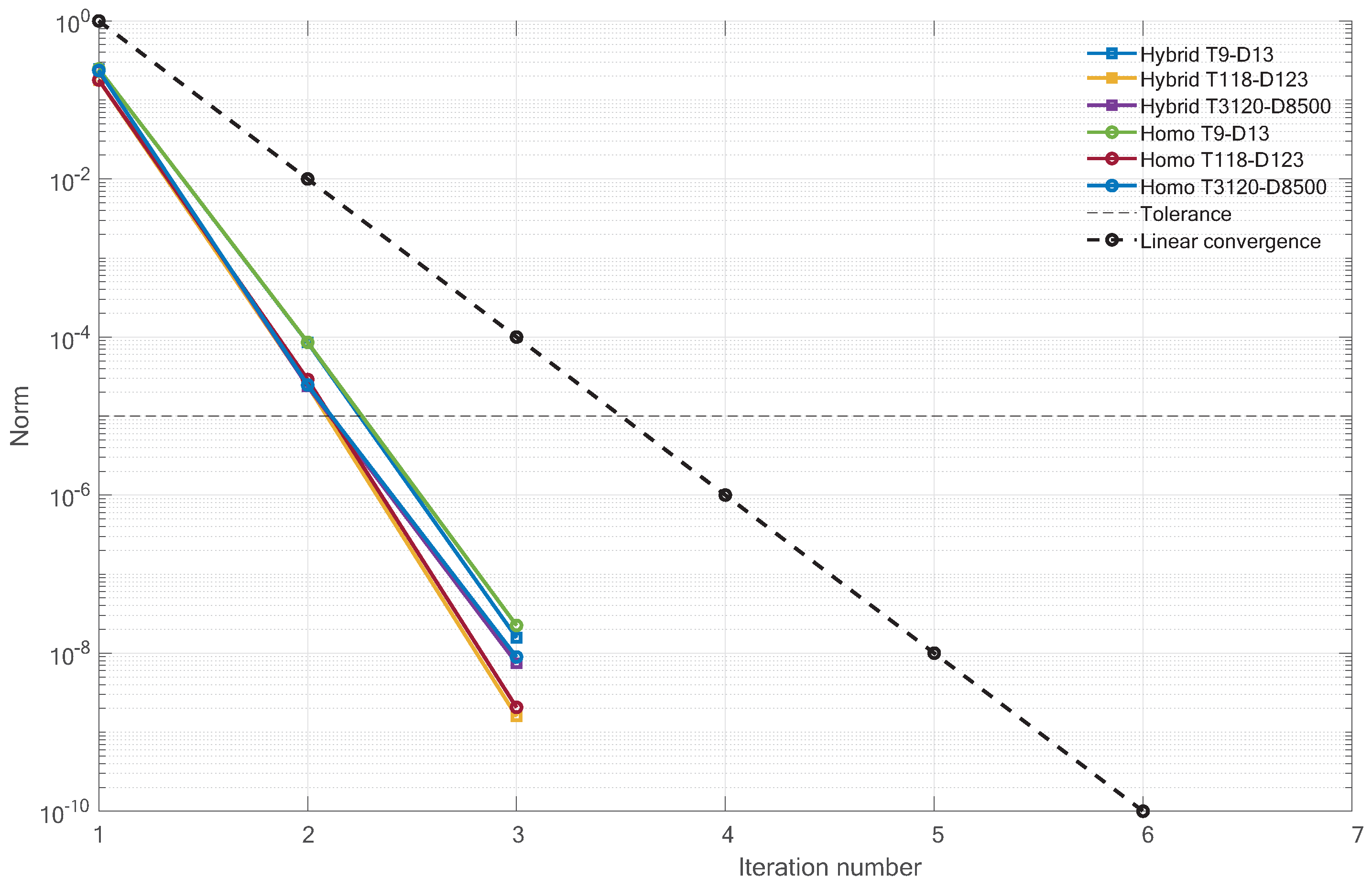
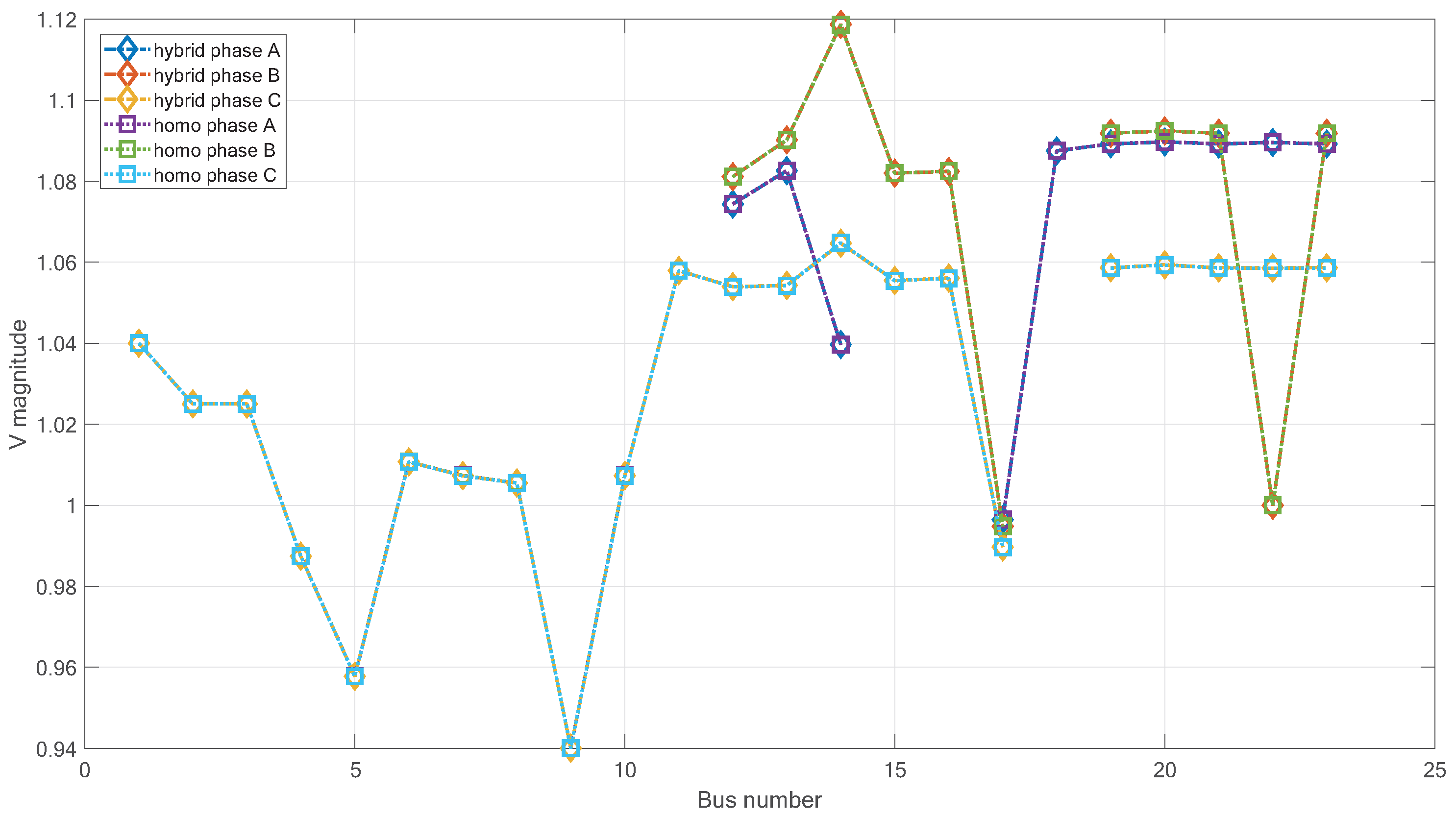
In this paper, we compared and assessed two types of stand-alone integration methods to solve the power flow problem. We classified them as unified and splitting methods and applied them to hybrid and homogeneous networks. This resulted in four different methods as the starting point of our comparison study and numerical assessment. We analyzed their accuracy and numerical performance—CPU time and number of iterations—using a Newton–Raphson solver together with an $LU$ factorization.

The numerical assessment showed that the unified methods are most favorable, which is in line with the expectations, stated in Section 3.3. As soon as the test cases become larger, the difference becomes more significant. Furthermore, it can be concluded that the methods applied to homogeneous networks take more CPU time than the methods applied to hybrid networks (1.5-times as much). The analysis of the addition of distributed generation and multiple distribution feeder showed that all the methods are relevant for real application.

Overall, it can be concluded that the interconnected method is the most favorable method at this moment, with the emphasis on this moment, because realistically sized networks have often multiple and larger distribution networks. The results between hybrid and homogeneous networks become then less significant. On top of that, these large networks require high-performance computing techniques such as Newton–Krylov methods and domain-decomposition techniques in a parallel or GPU environment. This makes the MSS methods more advantageous, although the developments for unified methods also continue in this field.

The current legislation determines the potential use case of the integration methods. In most countries, the usability of the unified methods is limited as complete network information is not allowed. The use of Newton–Krylov–Schwarz methods by the unified methods can help to share only the information of overlapping connecting buses between system operators, similar to the splitting methods. When system operators operate in geographically distinct locations, only the use of splitting methods is possible. The idea of the unified methods is still interesting for the analysis of separated networks where some imbalance occurs on certain lines of a merely balanced network.

As the developments in electricity network operation pushed by the energy transition are rapidly increasing the size and complexity of integrated power flow computations, we suggest focusing future work on efficient solvers such that the necessary computations can be performed in a reasonable amount of time. We list some concrete suggestions for future work. Firstly, regarding the unified methods, we recommend investigating in more detail which (combination of the) existing solvers are most efficient to solve integrated power systems and why, because the solvers that are currently used are built for separate load flow analysis. Secondly, we recommend to continue the study into iterative and parallel Newton–Krylov techniques for both the unified and splitting methods. As not much attention has been paid yet to these techniques, enough work can be performed on the adaptation of these techniques to integrated power flow computations. Finally, we suggest performing a similar numerical assessment of these techniques, but with more focus on the usability and applicability of these methods, as we expect that the numerical performance of these improved methods will become similar.