Dependence of Conjugate Heat Transfer in Ribbed Channel on Thermal Conductivity of Channel Wall: An LES Study

Abstract

A series of large eddy simulations was conducted to analyze conjugate heat transfer characteristics in a ribbed channel. The cross section of the rib is square and the blockage ratio is 0.1. The pitch between the ribs is 10 times the rib height. The Reynolds number of the channel is 30,000. In the simulations, the effect of the thermal resistance of the solid wall of the channel on convective heat transfer was observed in the turbulent flow regime. The numerical method used was based on the immersed boundary method and the concept of effective conductivity is introduced. When the conductivity ratio between the solid wall and the fluid (K*) exceeded 100, the heat transfer characteristics resembled those for an isothermal wall, and the cold core fluid impinging and flow recirculation mainly influenced the convective heat transfer. For K* ≤ 10, the effect of the cold core fluid impinging became weak and the vortices at the rib corners strongly influenced the convective heat transfer; the heat transfer characteristics were therefore considerably different from those for an isothermal wall. At K* = 100, temperature fluctuations at the upstream edge of the rib reached 2%, and at K* = 1, temperature fluctuations in the solid region were similar to those in the fluid region. The rib promoted heat transfer up to K* = 100, but not for K* ≤ 10. The Biot number based on the channel wall thickness appears to adequately explain the variation of the heat transfer characteristics with K*.

1. Introduction

Gas turbines are mainly used as prime movers for aircraft propulsion and natural gas power generation. Their thermal efficiency and output increase with their inlet temperature [1]. Current state-of-the-art turbine engines operate at inlet temperatures (1700 °C) well above the melting point of the material (1000 °C), and hence, the turbine blades are cooled by compressor bleed air (700 °C). Cooling air is supplied to the internal cooling passage of the turbine blade (Figure 1a), where ribs are installed to promote heat transfer. If the predicted temperature of the blade is out of 30 °C, the blade life can be halved, and therefore, local heat transfer by the rib and the blade temperature should be accurately predicted [2].

The effect of promoting heat transfer by using ribs has been studied under various conditions and by considering various variables over the past several decades. It has been reported that the channel blockage ratio, rib pitch (=p) [3], rib angle of attack [4], and rib shape [5,6] have a significant effect on performance. In the recirculating flow region behind the rib, heat transfer is not active. When the blockage ratio is increased, the pressure drop increases significantly, so the optimal values of blockage ratio and pitch exist [7]. It is recommended that the rib height (=e) be 10% of the channel height and the pitch be 10 times the rib height [8].

At a typical pitch of p/e = 10, since 90% of the channel wall is a bare surface, many studies have dealt with the heat transfer of the channel wall. Although rib heat transfer has received relatively little attention, on-rib heat transfer significantly contributes to the total heat transfer [6,9]. Most of the past studies have been performed under isothermal or iso-flux thermal boundary conditions [10]. In actual cooled turbine blades, solid conduction exists and is important for predicting the blade temperature [10,11]. In particular, heat transfer by the rib, where the conduction effect is concentrated, is not purely convective [12,13].

Iaccarino et al. [13] performed a Reynolds-averaged Navier–Stokes (RANS) simulation by adopting the k-ε v2f model and considering the conduction of the rib. They also imposed an iso-flux condition on the channel wall, despite conduction between the rib and the channel wall existing in actual cooled blades. Subsequently, studies conducted experiments on conjugate heat transfer including channel walls [14,15]. When conduction was considered, the average heat transfer coefficient decreased by 26% in the rib and 10% in the channel wall compared with the case of pure convection [15].

Using k-ε v2f improves [16], but in the ribbed channel problem, RANS underpredicts the heat transfer and does not accurately predict local peaks. Large eddy simulations (LESs) can solve these problems [17,18]. Furthermore, mechanisms for generating local peaks can be elucidated by observing instantaneous flow and thermal fields [18,19]. For studying the conjugate heat transfer of ribbed channels [14,15], Scholl et al. [20,21] performed a LES. The LES predicted that the heat transfer of the channel wall was in good agreement with the experiment, but the heat transfer coefficient at the front edge and back of the rib was higher than those observed in the experiment [20].

The difference observed between experimental and LES results at the edge of the rib indicates the possibility of an optical problem involving infrared camera images [22]. Additionally, the possibility of solid/fluid time disparity [23] caused by Scholl et al. [20,21] using the conduction–convection linkage as the heat transfer coefficient forward temperature back method was raised. Recently, Oh et al. [24] performed a fully coupled LES using the IBM (Immersed Boundary Method) for the same problem [13,14]. While the thermal response of a solid and a fluid has been shown to affect temporal changes in the temperature, it does not significantly affect the time-averaged heat transfer [24].

In the above studies [14,15,20,21,24], the blockage ratio was 0.3 and the thickness of the channel wall was the same as the rib height. In actual turbine blades, the typical blockage ratio is about 0.1, and the wall thickness is usually 2 to 7 times the rib height [25,26]. Ahn et al. [27] performed a fully coupled LES of a ribbed channel with a blockage ratio of 0.1 by applying the IBM. They also set the channel wall thickness to be thrice the ribs to consider an appropriate length scale when defining the Biot number (Bi). They found that Bi was below 0.1, and the amount of reduction in the conjugate heat transfer compared with pure convection was predicted to be 3%.

The reasons for the effect of conduction being small (3%) are the blockage ratio and the thermal conductivity of the blade material, which is 500 to 600 times that of air [27]. On the basis of dimensional analysis, Cukurel and Arts [15] showed that the heat transfer characteristics of a ribbed channel with a conducting wall can be expressed as

Nu = f(Re, K*, Bi),

(1)

where the thermal conductivity ratio K* (=k_s/k_f) is important for conjugate heat transfer. The blade material and coolant (air) are predetermined and therefore not actively considered. Recently, as 3D printing has been reviewed as a production technique for turbine blades [28,29], it has become possible to have a turbine blade with different thermal conductivities. Recently, as a new gas turbine cycle [30,31] has been studied as a countermeasure against global warming, cooling fluids with thermal conductivities different from that of air, such as carbon dioxide and water vapor, are being studied [32,33].

The effect of the thermal conductivity ratio has been partially addressed in previous studies related to ribbed channels. Iaccarino et al. [13] compared cases with K* = 0.1, 1, and 100, but their results were RANS results and they did not consider wall conduction. Oh et al. [24] only verified their code for laminar flow over a flat plate in the range of K* = 0.01 to 1, and they did not report the effect of K* in the ribbed channel. In the current study, we observed the effect of the thermal conductivity ratio on the turbulent heat transfer of the ribbed channel for K* = 1, 10, 100, and 566.26.

In this study, a channel wall with a thickness thrice the rib height was considered in the calculation area and a fully coupled LES was performed using the IBM. The thermal conductivity ratio was analyzed for 1, 10, and 100 cases with 566, which is a typical value for a gas turbine blade, and the results were compared. On the basis of the time average temperature field and heat transfer distribution, it was examined whether the mechanism responsible for promoting heat transfer under pure convection conditions is valid even when the conductivity ratio is different. Furthermore, conjugate heat transfer characteristics for different K* values were observed through the instantaneous flow and thermal fields. Finally, the thermal performance of a ribbed channel according to the thermal conductivity ratio and the Biot number is discussed.

2. Numerical Methods

In the simulation, an in-house code was used. This code was based on the finite volume incompressible Navier–Stokes solver [31] at Stanford University, USA. All spatial derivatives were discretized by the central difference with second-order accuracy. The semi-implicit fractional step method based on the Crank–Nicolson and Runge–Kutta methods with third-order accuracy was used as the time integration method. The code was revised to deal with solids in the flow field with the IBM [32] and supplemented to solve the convective heat transfer between solids and fluids [33]. Later, it was revised twice, once to perform an LES of turbulent heat transfer [18,19], and again to handle conjugate heat transfer (CHT) [34].

The computational domain analyzed in this study is presented in Figure 1b. Ribs with a square cross-section and a height (e) that was 0.1 of the channel height (H) are arranged at intervals of 10 e on the upper and lower sides of the channel. By comparing the computational domain, including three periods in the x direction and one including single period, the same time average result was obtained, and finally, the computational area was set to include single period as shown in Figure 1c. The spanwise domain was set to be 2.5 π e, for which zero fall-off was observed with two-point correlation in a smooth channel simulation [18,19]. The thickness of the solid wall was set to be three times e, which corresponds to 30% of H.

Periodic boundary conditions were imposed in the main flow (x) and spanwise (z) directions. In the wall normal direction (y), no slip conditions or isothermal conditions were imposed on the upper and lower surfaces in the computational domain. The grid system comprised 128, 256, and 48 meshes in the x, y, and z directions (Figure 1c). A nonuniform grid was used in the x and y directions, while a uniform grid was used in the z direction. This was similar to the resolution obtained by [35] for a grid independent solution by performing a resolution test on the LES of a ribbed duct.

The grid-filtered incompressible Navier–Stokes equation and energy equation were adopted as the dimensionless governing equations, and they can be expressed as follows [34]:

$$\frac{\partial {\overline{u}}_i}{\partial x_i}-ms=0,$$

(2)

$$\frac{\partial {\overline{u}}_i}{\partial t}+\frac{\partial {\overline{u}}_i{\overline{u}}_j}{\partial x_j}=-\frac{d\overline{p}}{d{x}_i}+\frac{1}{\mathrm{Re}} \frac{{\partial }^2{\overline{u}}_i}{\partial x_j\partial x_j}+\frac{\partial {\tau }_{ij}}{\partial x_j}+f_i,$$

(3)

$$\frac{\partial \overline{\theta }}{\partial t}+\omega \frac{\partial }{\partial x_j}\left({\overline{u}}_j\overline{\theta }\right)= \frac{C^{\ast }{K}^{\ast }}{\mathrm{Re} \mathrm{Pr}}\frac{{\partial }^2\overline{\theta }}{\partial x_j\partial x_j}+ \frac{\partial q_j}{\partial x_j}+\xi .$$

(4)

Under the assumption of fully developed flow, the mean streamwise pressure and temperature gradient were decoupled as follows to impose periodic boundary conditions in the streamwise direction [36]:

P(x, t) = −βx + p(x, t),

(5)

T(x, t) = γx + θ(x, t),

(6)

where β and γ are the mean streamwise pressure and temperature gradients, respectively. These two parameters were determined to satisfy the conservation of global momentum and energy, respectively [36].

In the energy equation, the thermal properties of the solid were distinguished from those of the fluid by defining the heat capacity ratio C* and the thermal conductivity ratio K*, and by introducing the concept of effective thermal conductivity (k_e). The effective thermal conductivity was determined to satisfy the continuity of temperature and heat flux at the interface [34]. The parameter ω was a convection correction factor, and it was 0 in the cell containing the solid–fluid boundary and 1 in the remaining cells when conduction between the solid and the fluid was considered. In Equation (4), ξ was introduced to maintain second-order accuracy in the cell containing the interface [34]. The code was verified through the CHT problem involving a ribbed duct and a circular cylinder [34].

Turbulent flow was analyzed using an LES. In Equations (3) and (4), τ_ij and q_j are the sub-grid scale turbulent stress and turbulent heat flux, respectively, and τ_ij was determined as a dynamic sub-grid model by using scale similarity and setting a test filter around the grid [37,38]. The dynamic sub-grid model provided better results than the constant model for the ribbed channel problem [35]. Similar to τ_ij, q_j was determined dynamically; this approach yields better results in problems where the flow and heat transfer are dissimilar [39]. The simulation were performed for 10,000 time steps to reach a steady state. After that, additional 10,000 time steps (t U_b/D_h = 5) were carried out to obtain the statistics.

Numerical analysis was performed with thermal conductivity ratios of 1, 10, 100, and 566.26 to examine the thermal resistance effect of the solid wall. The value 566.26 is the thermal conductivity ratio between the gas turbine blade material and air [22]. The remaining flow and geometry conditions are summarized in

Table 1. Parameters related to conjugate heat transfer.

	Present Study	Liou et al. [6]	Cukurel et al. [14,15]	Scholl et al. [20,21]
Method	LES	Hologram	IR Camera	LES
Re	30,000	10,200	40,000	40,000
Pr	0.71	0.71	0.71	0.71
K*	566.36	1368.8	618.32	618.32
C *	0.00031	0.00038	0.00031	0.00031
d/e	3	0.75	1	1

. In this study, an LES was performed to obtain the instantaneous flow field and turbulence statistics along with the time average flow and temperature field. Furthermore, the turbulent heat transfer on the fluid side and changes in temperature fluctuations on the solid side according to the thermal conductivity ratio were observed.

3. Results and Discussion

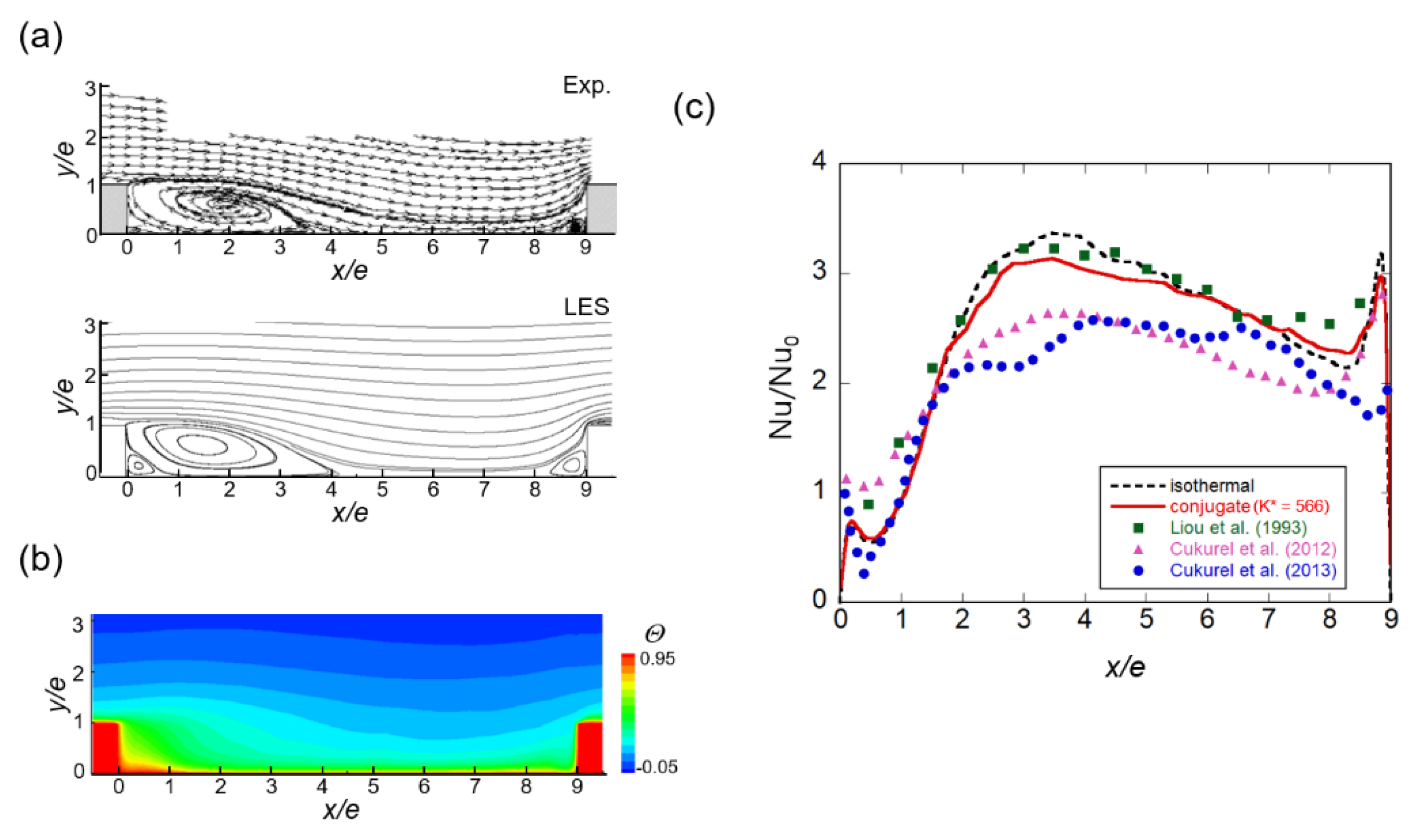
3.1. Code Validation Study

Figure 2a shows the time-averaged streamline in the ribbed channel. Similar to the streamlines [40] obtained with experimental data, recirculating cells exist behind the rib, and there is a secondary vortex between the recirculation flow and the back of the rib. There is a vortex on the front side of the rib and there is a separation bubble on the top side of the rib. While the LES-predicted flow field was almost identical to that observed in the experiment, the corner vortices occurring before and after the rib were predicted to be slightly larger compared with those in the experiment. This appears to be because of the difference between the blockage ratio and the channel aspect ratio. In the time-averaged temperature distribution under isothermal conditions (Figure 2b), a high-temperature region was formed behind the rib since heat transfer was not active.

Figure 2c shows a comparison of the heat transfer coefficient distribution at the channel wall with those in the literature (see Table 1). The heat transfer coefficient was compared with the Nusselt number ratio, where Nu₀ is the Nusselt number of a smooth channel wall obtained using the following Dittus–Boelter correlation:

$$N{u}_0=0.023 R{e}^{0.8} P{r}^{0.4}.$$

(7)

When wall conduction was considered (red solid line in Figure 2c), the local heat transfer change slightly decreased compared with that obtained through locally isothermal analysis (black dotted line in Figure 2c). Among the experimental data, it was in good agreement with that of Liou et al. [6] (green square), who adopted the same blockage ratio (=0.1). The results of Cukurel et al. [14,15] compared together had a blockage ratio of 0.3, and the pink triangle and blue circle show iso-flux and conjugate results, respectively. Although not as quantitatively consistent as [6], the tendency of the convective heat transfer to be higher than the conjugate heat transfer in the range of 2 < x/e < 4 and the reversal of this tendency downstream are identical to those in the present study.

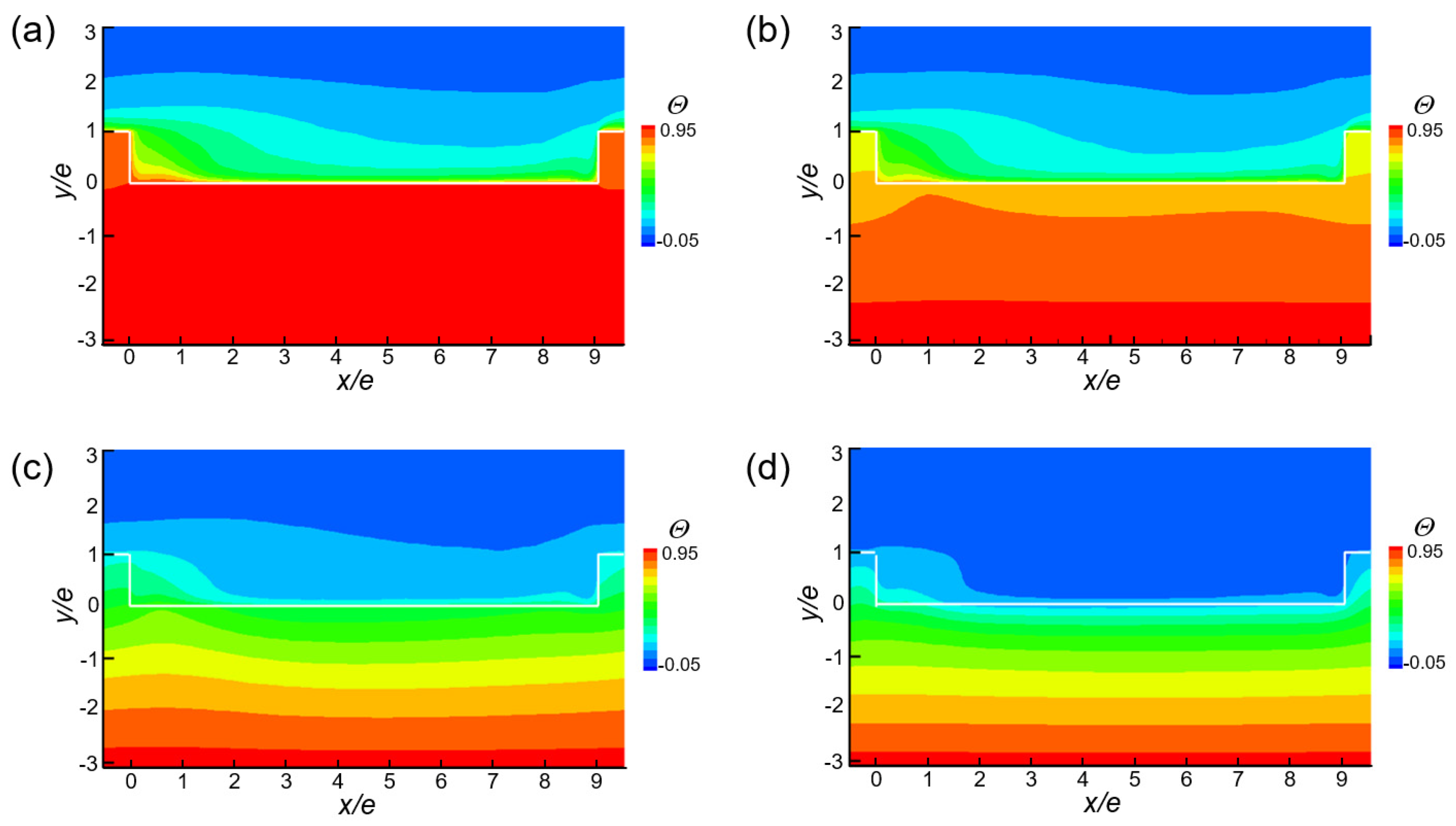
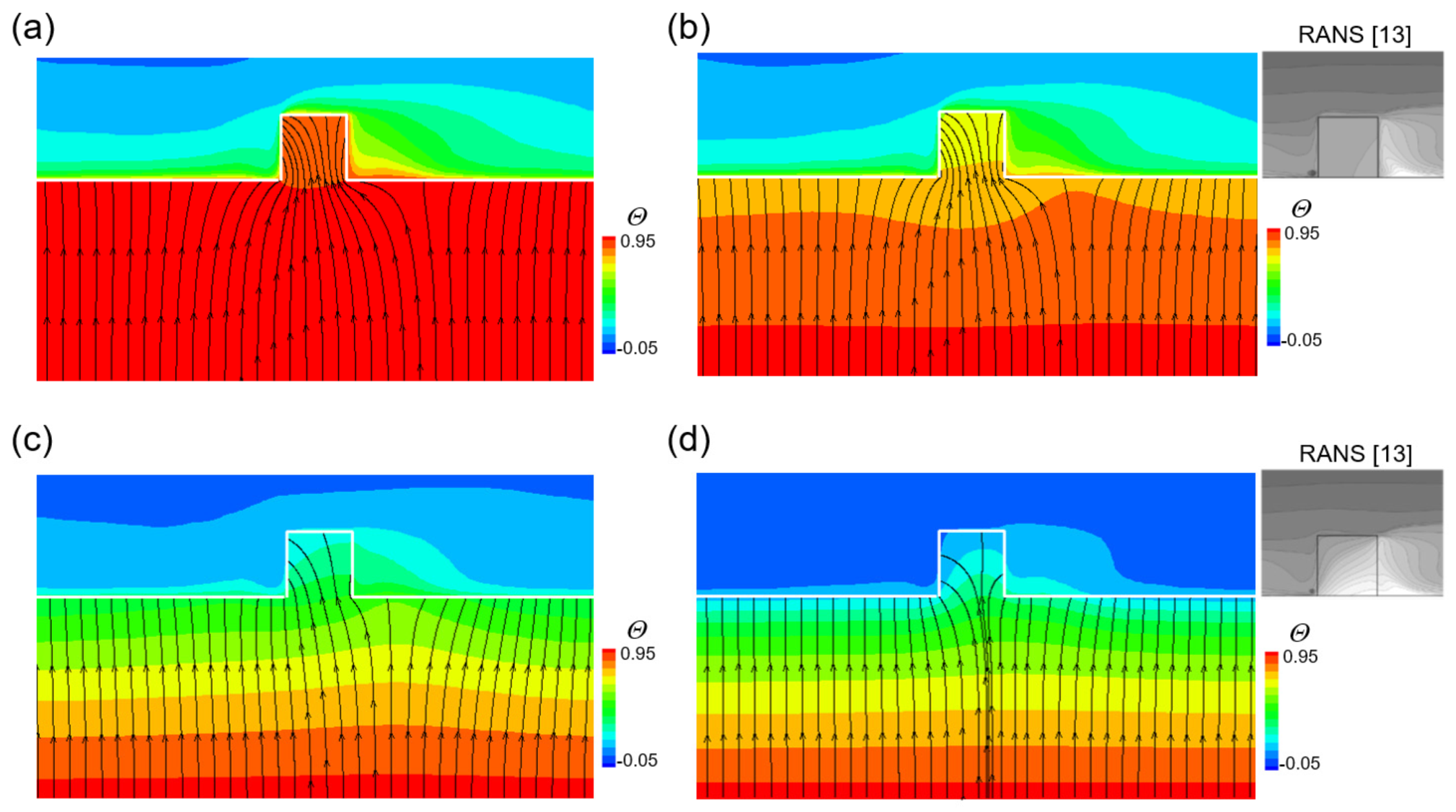
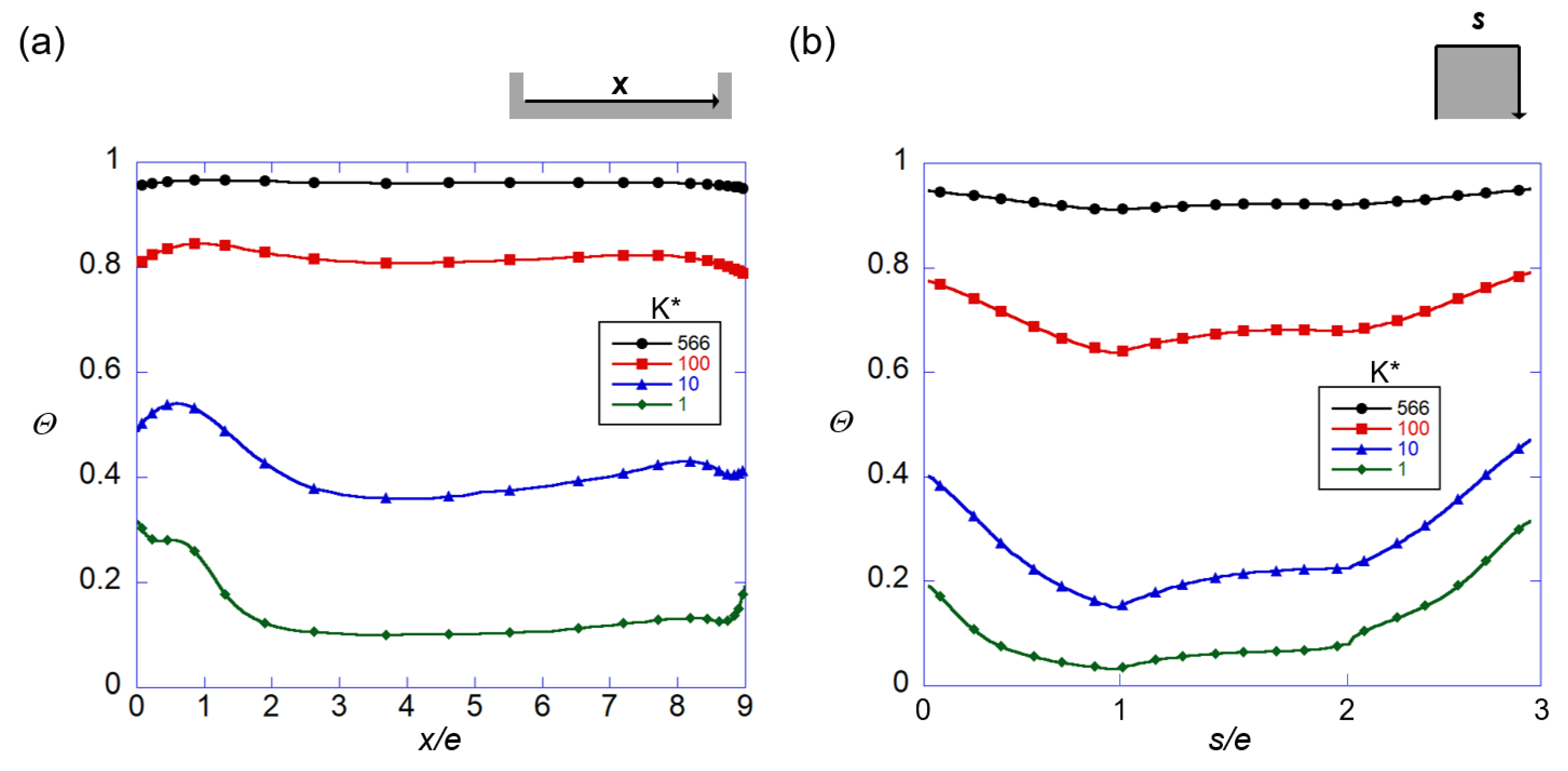
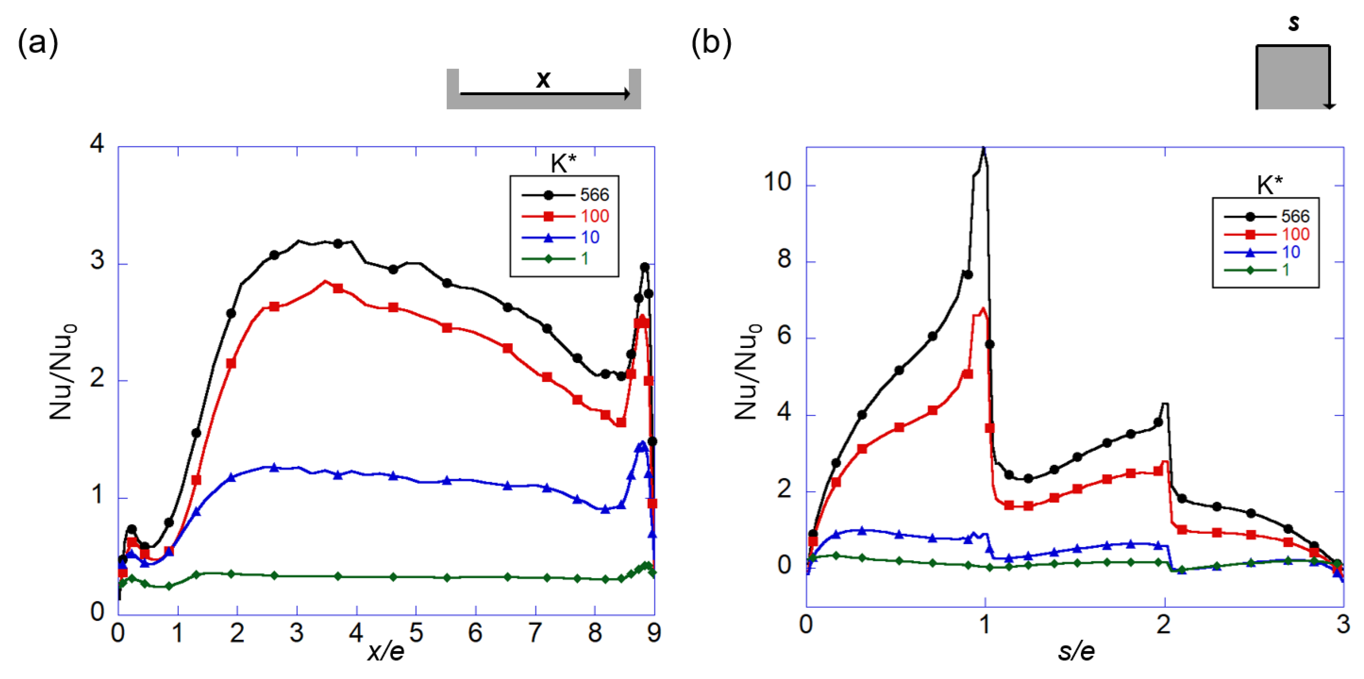
3.2. Time-Averaged Thermal Fields and Heat Transfer

The time-averaged temperature fields for different thermal conductivity ratios (K*) are compared in Figure 3. For a high conductivity ratio (K* ≥ 100), the temperature distributions are similar to those for the isothermal wall condition (Figure 3a,b). The fluid region accounts for most of the thermal resistance, and therefore, the temperature distribution inside the solid wall is uniform and the temperature in the fluid region near the solid–fluid interface varies.

On the other hand, in the case of low conductivity ratios (K* ≤ 10), the contour lines are narrowly packed in the solid region and the temperature distribution in the fluid region is relatively uniform since the thermal resistance inside the solid wall is greater than that of the fluid (Figure 3c,d).

Figure 4 shows the heat flux inside the solid wall for each thermal conductivity ratio; the contours are isotherms. In general, the thermal resistance of a fluid varies greatly spatially because of the recirculation of the flow and the collision of the cold core fluid [18,19]. On the other hand, the thermal resistance inside the solid wall is constant. When the thermal conductivity ratio is large (K* ≥ 100), the thermal resistance in the fluid dominates. Therefore, the heat flux vector inside the solid wall is concentrated on the rib and directed toward both edges of the rib (Figure 4a,b).

When the thermal conductivity ratio is small (K* ≤ 10), the thermal resistance inside the solid wall is dominant. Consequently, the heat flux vector flows toward the fluid in the wall normal direction (y), without being concentrated on the rib. In Figure 4c,d, the heat flux vector inside the rib is toward the upstream edge. However, the heat flux is smaller than that for a large thermal conductivity ratio. Furthermore, when the thermal conductivity ratio is 10 (Figure 4c), the fluid temperature is higher than that of the rib on the downstream side of the rib, and therefore, the heat flux cannot pass through the rib.

The cases of K* = 100 and 1 were compared with RANS data [13] by adopting the same thermal conductivity ratio. At K* = 100 (Figure 4b), the temperature inside the rib was almost uniform for both LES and RANS simulation. In the present LES, the isotherm inside the rib including the channel wall was close to the horizontal line, but in the RANS simulation in which only the conduction of the rib was considered, the isotherm inside the rib appeared in the diagonal direction. At K* = 1, both LES and RANS simulation increased the number of isotherms inside the rib. The number of isotherms of the LES including the channel wall was considerably smaller than that of the RANS simulation. In the RANS simulation, isotherms occurred in a diagonal direction, while in the LES, they occurred in the form of a parabola that was convex upwards. If K* = 100 or less, the conjugate effect can be accurately identified only when the channel wall is included in the computational domain.

Figure 5 shows the dependence of local temperature distributions at the solid–fluid interface on the thermal conductivity ratio. In the case of high conductivity ratios (K* ≥ 100), the temperature at the interface between the ribs (Figure 5a) is considerably close to the outer wall temperature and uniform in space since the solid wall tends to maintain a uniform temperature distribution. Similar behavior is observed on the rib surface (Figure 5b). However, the upstream edge of the rib has the lowest temperature because of the high heat transfer rate. This is clearly observed for K* = 100.

In the case of low conductivity ratios (K* ≤ 10), the temperature was considerably lower than that in the case of high conductivity ratios, and a relatively large temperature variation was observed. The reason is that the spatially nonuniform thermal resistance of the flow field mainly influenced the temperature at the interface. In particular, the temperature near the upstream corner of the rib increased (Figure 5a). For K* ≤ 10, the fluid impinging on the upstream face of the rib was not very cold compared with the solid wall. However, the corner vortex prevented heat transfer from the solid to the fluid, resulting in the temperature near the upstream corner of the rib increasing.

Figure 6 shows the effect of the thermal resistance of the solid wall on the local heat transfer. Nu₀ is the Nusselt number without ribs, given by Equation (7). The Nusselt number presented in Figure 6 was defined on the basis of D_h. In Figure 6a, the local heat transfer coefficient evidently increases (8 ≤ x/e ≤ 9) near the upstream corner for all thermal conductivity ratios as the cold core fluid collides with the rib. However, as the thermal conductivity ratio increases, the local heat transfer coefficient decreases noticeably and becomes spatially uniform. Quantitatively, the local heat transfer coefficient depends strongly on the thermal conductivity ratio, but its qualitative distribution does not significantly depend on the local thermal conductivity ratio. Except in the vicinity of the rib, heat conduction in the flow direction is not significant since the heat flux vector inside the solid is directed in the +y direction (Figure 4).

On the other hand, the local heat transfer distribution over the rib was strongly dependent on the thermal conductivity ratio (Figure 6b). Quantitatively, even at K* = 566.26, the heat transfer rate at both edges of the rib was considerably lower than that in the isothermal case, and the local difference was quite small. Nevertheless, for large thermal conductivity ratios (K* ≥ 100), the distribution of local heat transfer was qualitatively similar to that of the isothermal wall. However, when the thermal conductivity ratio became small (K* ≤ 10), the heat transfer distribution changed qualitatively. For large thermal conductivity ratios, the maximum value of heat transfer occurred at the upstream edge of the rib, while for small thermal conductivity ratios, the maximum value of heat transfer occurred near the upstream edge of the rib (s/e ≈ 0.2). Furthermore, in the vicinity of the downstream edge (s/e ≈ 2.1), as the temperature of the solid decreased below that of the fluid, a region with negative heat transfer was formed.

3.3. Turbulent Heat Transfer

Figure 7 shows turbulent heat flux contours. It is well known that turbulent heat flux is an important factor in determining heat transfer [18,19]. The turbulent heat flux was large near the two edges of the rib and around x/e = 4 near the wall. For all heat flux ratios, the distribution of turbulent heat flux was similar, but when the thermal conductivity ratio decreased, the value of turbulent heat flux decreased and the distribution of turbulent heat flux became spatially uniform. As shown in Figure 3, when the heat conduction ratio decreased, the temperature distribution on the fluid side became uniform and the turbulent heat transfer decreased. In particular, the peak of the turbulent heat flux near the wall disappeared for K* < 10.

Locally, the turbulent heat flux near the rib varied with the thermal conductivity ratio. As evident in Figure 7a,b, when the thermal conductivity ratio was large, the turbulent heat flux at the front face of the rib was almost uniform. On the other hand, when the thermal conductivity ratio was small, the effect of the corner vortex relatively increased, resulting in the turbulent heat flux at the corner exceeding that at the edge. Consequently, the heat transfer distribution near the rib varied with the thermal conductivity ratio (Figure 6).

Figure 8 shows temperature fluctuations inside the solid wall. As explained in the introduction, the thermal condition of the solid wall is an important factor in determining convective heat transfer. In particular, in the turbulent flow section, temperature fluctuations in the solid are important along with thermal resistance. When the thermal conductivity ratio exceeds 1, most temperature fluctuations are caused by turbulent flows in the fluid region. At K* = 100, the temperature fluctuation at the upstream edge of the rib reaches 2%. When K* is 10 or higher, the temperature fluctuation inside the solid increases with the thermal resistance of the solid. When the thermal conductivity ratio is 1, the effect of the flow on convective heat transfer decreases and the temperature fluctuation in the fluid region weakens. Consequently, the temperature fluctuation in the solid region becomes similar to that in the fluid region. Furthermore, the depth at which temperature fluctuations occur inside the solid becomes smaller than that for K* = 10 or 100. When the thermal conductivity ratio is 1, the influence of the corner vortices becomes significant, and therefore, the maximum temperature fluctuation occurs at the corners of the rib.

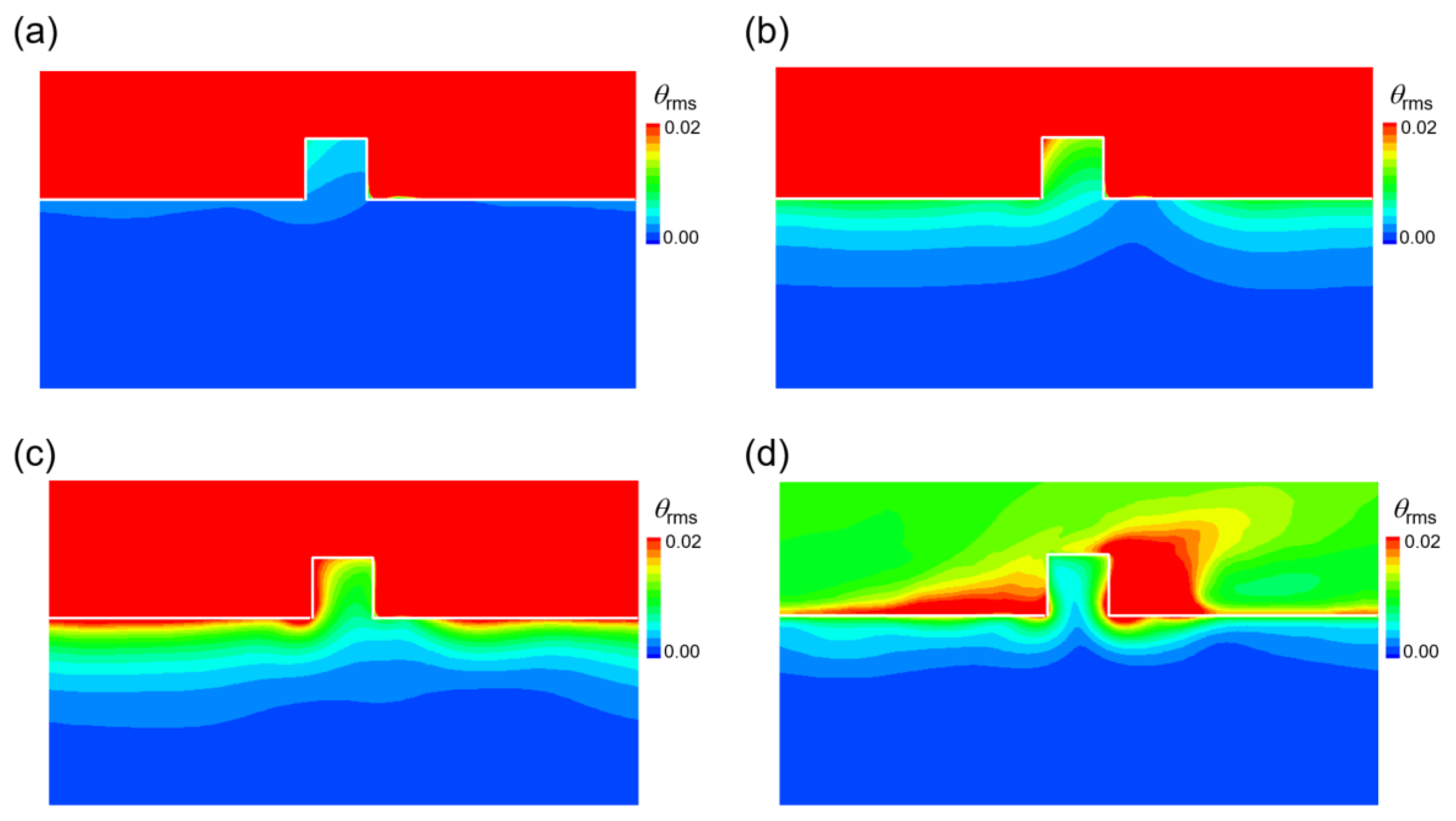
3.4. Instantaneous Thermal Fields

Figure 9 shows instantaneous temperature fields near the rib. When the thermal conductivity ratio was large, the temperature inside the solid wall exceeded that of the fluid at all interfaces (Figure 5). In those cases, the difference between the bulk temperature of the fluid and the temperature on the solid surface was large (Figure 5), and therefore, the cold core fluid impinging became an important heat transfer mechanism.

However, as the thermal resistance of the solid increased (K* ≤ 10), the temperature difference between the fluid and the solid decreased. Consequently, the impingement of the fluid did not significantly influence the convective heat transfer in the near-upstream region of the rib. In this case, the corner vortex at the upstream corner of the rib induced a temperature change and reduced the local thermal resistance, resulting in the convective heat transfer increasing near both corners of the rib. In particular, the effect of the secondary vortex generated after the rib was very different when the thermal conductivity ratio was small. As shown in Figure 9c, the fluid heated by the channel wall was supplied to the downstream face of the rib by the recirculation flow and the secondary vortex. Consequently, the heat transfer rate at the downstream face of the rib was negative. In the temperature field of Figure 9d, compared with the temperature field of Figure 9c, it is evident that the isotherms are more concentrated near the surface as the relative thermal resistance of the solid increases. Consequently, the top surface of the rib is not heated and remains cold, and the cold flow over the rib takes heat from the rib and the hot fluid behind the rib.

Figure 10 shows the local heat transfer distribution obtained for the instantaneous temperature field. Here, A, B, C and D represent the upstream corner, upstream edge, downstream edge, and downstream corner of the rib, respectively. At K* = 566.26, the cold fluid flowing along the wall collides with the rib, greatly promoting heat transfer to the upstream face of the rib. This can be confirmed by the repeated occurrence of high heat transfer after the corner at the location of the streak with a high heat transfer coefficient on the channel wall based on A, which corresponds to the upstream corner of the rib. At edge B, as the flow separates and recombines, spots with high heat transfer coefficient occur on the downstream side of the top of the rib. The downstream face of the rib is partially supplied with recombined cold fluid and has a high heat transfer coefficient, but the overall heat transfer is greatly reduced compared with the upstream face. In the downstream corner D, a locally negative heat transfer coefficient (white area in the contour) is observed. For K* = 100, the above-mentioned trend is maintained, but the heat transfer coefficient is reduced overall.

As the thermal conductivity ratio decreases (K* ≤ 10), the heat transfer rate decreases and becomes uniform overall. As the heat transfer rate decreases, the area of negative heat transfer (the white area in Figure 10) also widens. In the case of K* = 10 (Figure 10c), a negative heat transfer coefficient appears on the downstream side and along the downstream corner (D). For K* = 1, it appears along the downstream corner (C) but not at the downstream corner. This appears to be because the cold fluid flowing over the top of the rib cools the rib, as discussed in the context of Figure 9.

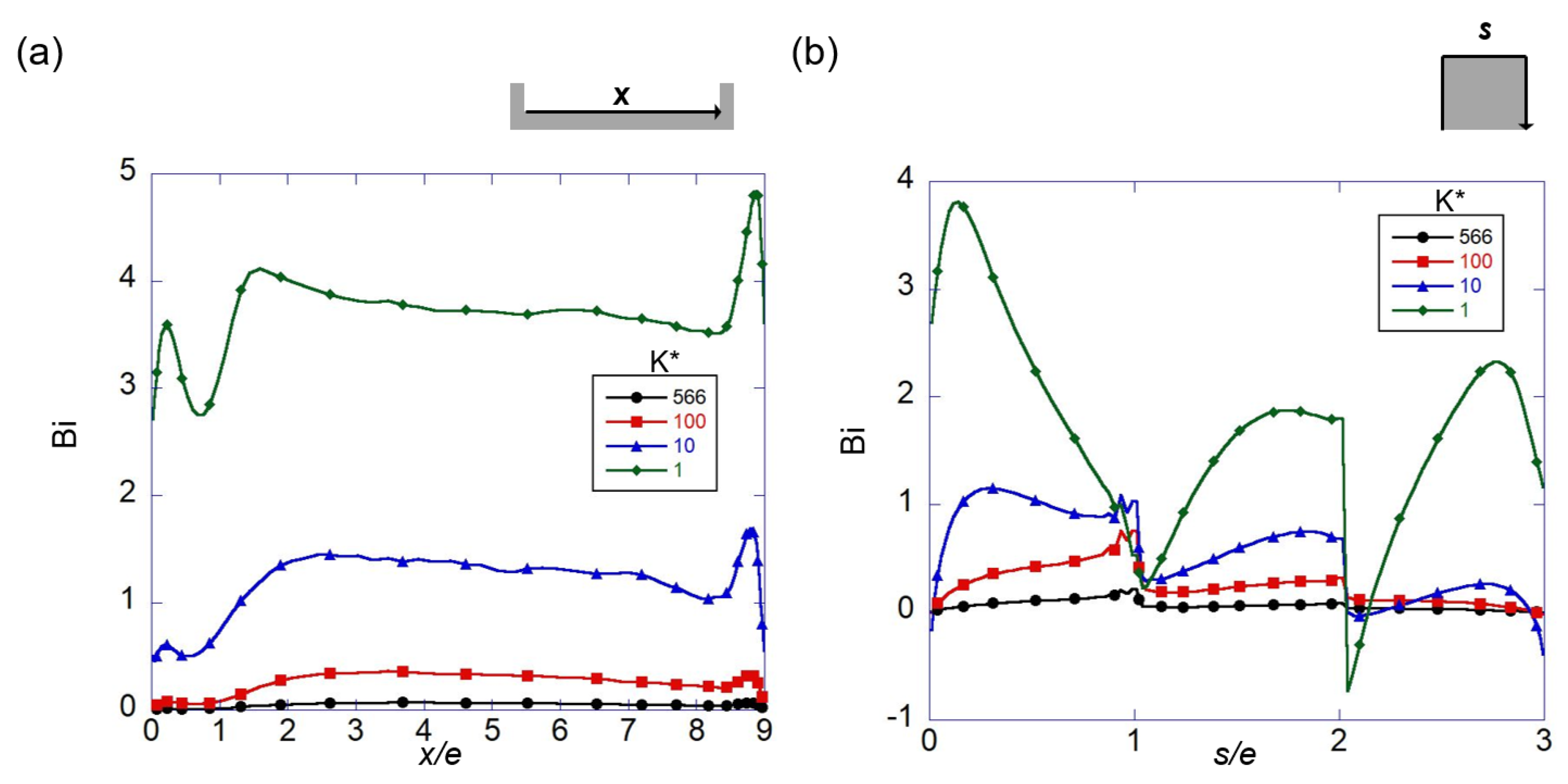
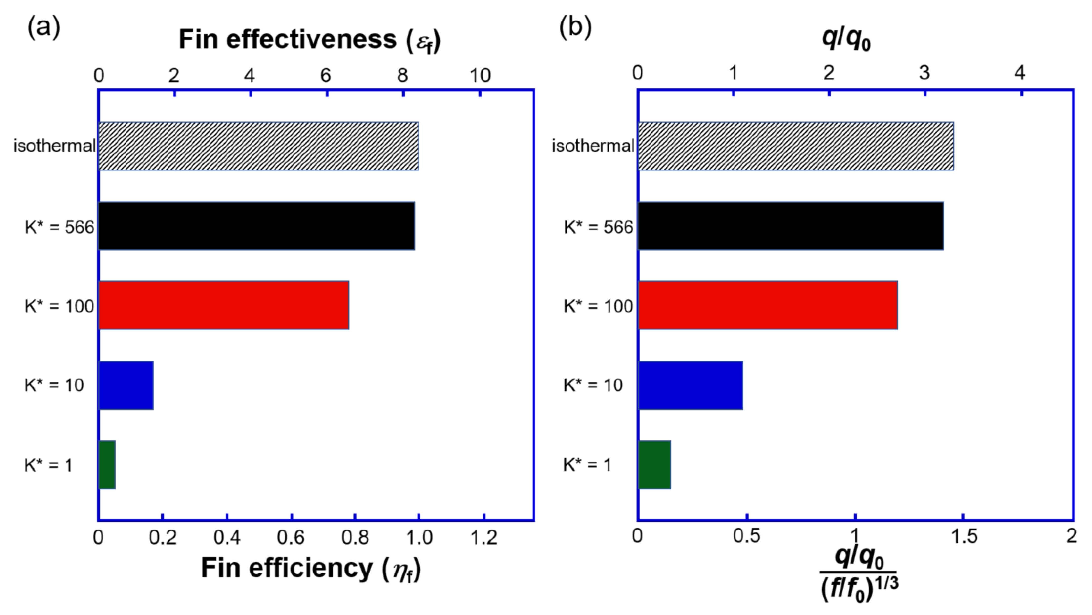
3.5. Thermal Performance and Biot Number

Since ribs can be considered to be extended surfaces or fins, the performance of fins was analyzed. Fin performance is evaluated by examining the fin effectiveness and fin efficiency [41]. The fin effectiveness is defined as follows:

$${\epsilon }_f=\frac{q_{rib,conj}}{h_{conv}{A}_{c,b}\left(T_w-T_b\right)}.$$

(8)

Fins are judged to be effective when their effectiveness is 2 or more [41], and this condition is satisfied when K* is 100 or higher (see Figure 11a).

The fin efficiency is defined as follows [41]:

$${\eta }_f=\frac{q_f}{q_{max}}=\frac{q_{rib,conj}}{h_{conv}{A}_{rib}\left(T_w-T_b\right)}.$$

(9)

Since numerator is identical to q_rib,conj, it shows the same trend as the fin effectiveness. In actual gas turbine materials (K* = 566), the fin efficiency is close to 100%, but at K* = 100 it decreases to 78%. At K* = 10, the fin efficiency is less than 20%, and the fin does not perform its intended function properly.

The total heat transfer rate (q) is shown in Figure 11b; q₀ is the heat transfer rate in the smooth channel for pure convection, and it is obtained from the Dittus–Boelter equation (Equation (7)). Figure 11b shows that the overall heat transfer rate decreases significantly as K* decreases. For K* = 566.26, there is no significant difference from the isothermal conditions, but for K* = 100, the overall heat transfer rate decreases by about 17%. At K* = 10, it is less than 1/3, and at K* = 1 it is considerably smaller than that in the isothermal smooth channel.

Thermal performance considering both heat transfer and pressure drop is defined by Equation (10), where f stands for frication factor [10].

$$\mathrm{Thermal} \mathrm{performance}=\frac{q/q_0}{{\left(f/f_0\right)}^{1/3}}.$$

(10)

Thermal performance is proportional to the total heat transfer rate as the flow field (i.e., friction factor) does not change even when the conductivity changes. For the heat transfer enhancement to be greater than the pressure drop penalty, the value of thermal performance should exceed 1, but this criterion is satisfied only when K* = 100 or higher. If K* = 10 or lower, the rib is not effective in promoting heat transfer.

Figure 12 shows the variation of the local Biot number with the conductivity ratio. The Biot number on the coolant side, which is within the scope of this study, is defined by Equation (11), using the thickness of the solid wall (d) as the characteristic length [42]:

$$\mathrm{Bi}=\frac{h_{conj}d}{k_{\mathrm{s}}}=\frac{\mathrm{Nu}}{K^{\ast }}\frac{d}{D_h}.$$

(11)

In a cooled gas turbine blade, Bi is typically around 0.3 [43]. If the Biot number is less than 0.1, the fluid domain accounts for most of the thermal resistance, similar to the isothermal case [43]. Ahn et al. [27] reported that under typical gas turbine blade conditions, the Biot number is less than 0.1 (black circles in Figure 12) and reflects heat transfer characteristics close to pure convection.

At K* = 100 (red squares), Bi exceeds 0.1 at 3 < x/e < 6 on the channel wall, making the conduction thermal resistance non-negligible (Figure 12a), and at the rib surface, Bi goes up to 0.6 at the upstream edge (Figure 12b). At K* = 10 (blue triangles), Bi is close to 1, and the thermal resistance of the solid is similar to that of the fluid. About half of the temperature drop is expected in the solid region. The data for K* = 10 in Figure 5 shows that θ is around 0.4, confirming that the Biot number is an appropriate indicator. At K* = 1 (green diamonds), Bi exceeds 1 in most regions, resulting in a higher temperature drop in solids than in fluids, consistent with the results presented in Figure 3, Figure 4 and Figure 5.

4. Conclusions

In this study, a CHT analysis including heat conduction in a ribbed channel was performed, and the effect of the thermal resistance of a solid wall was discussed on the basis of simulation data. The main results can be summarized as follows.

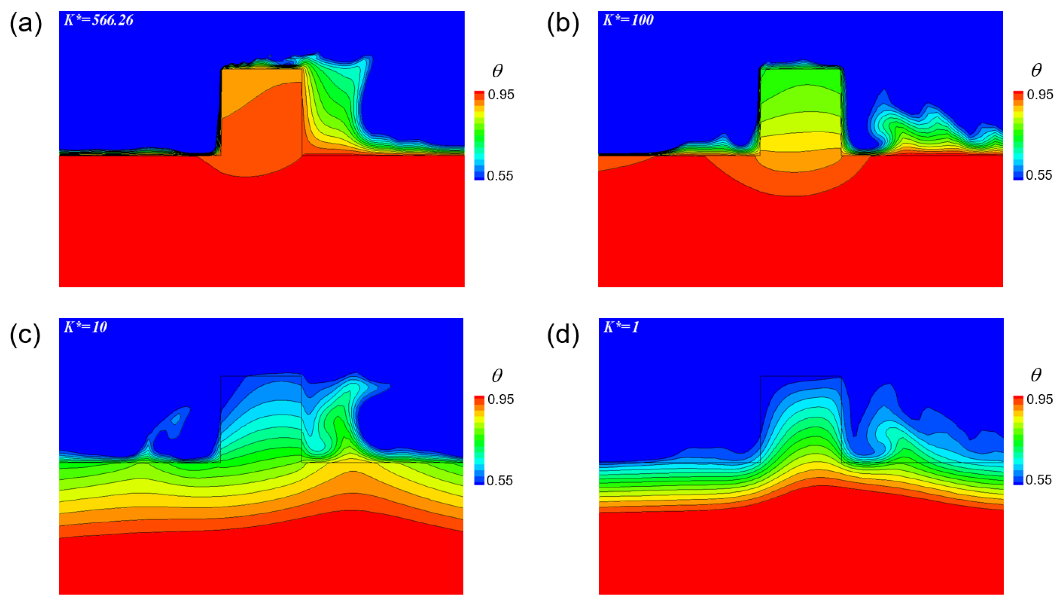
• When the thermal conductivity ratio was large (K* ≥ 100), the heat transfer characteristics were similar to those in isothermal conditions. In this case, the impingement of the cold core fluid into the rib and recirculation of the flow mainly affected the convective heat transfer. The heat flux from the solid wall was concentrated on the rib and directed toward both edges of the rib.
• When the thermal resistance of the solid increased (K* ≤ 10), the effect of cold core fluid impingement on the rib decreased, and the two vortices located at the corners played an important role in heat transfer. In this case, the temperature distribution of the solid wall that was affected by the two corner vortices determined the convective heat transfer. In particular, on the downstream face of the rib, a region with negative heat transfer appeared.
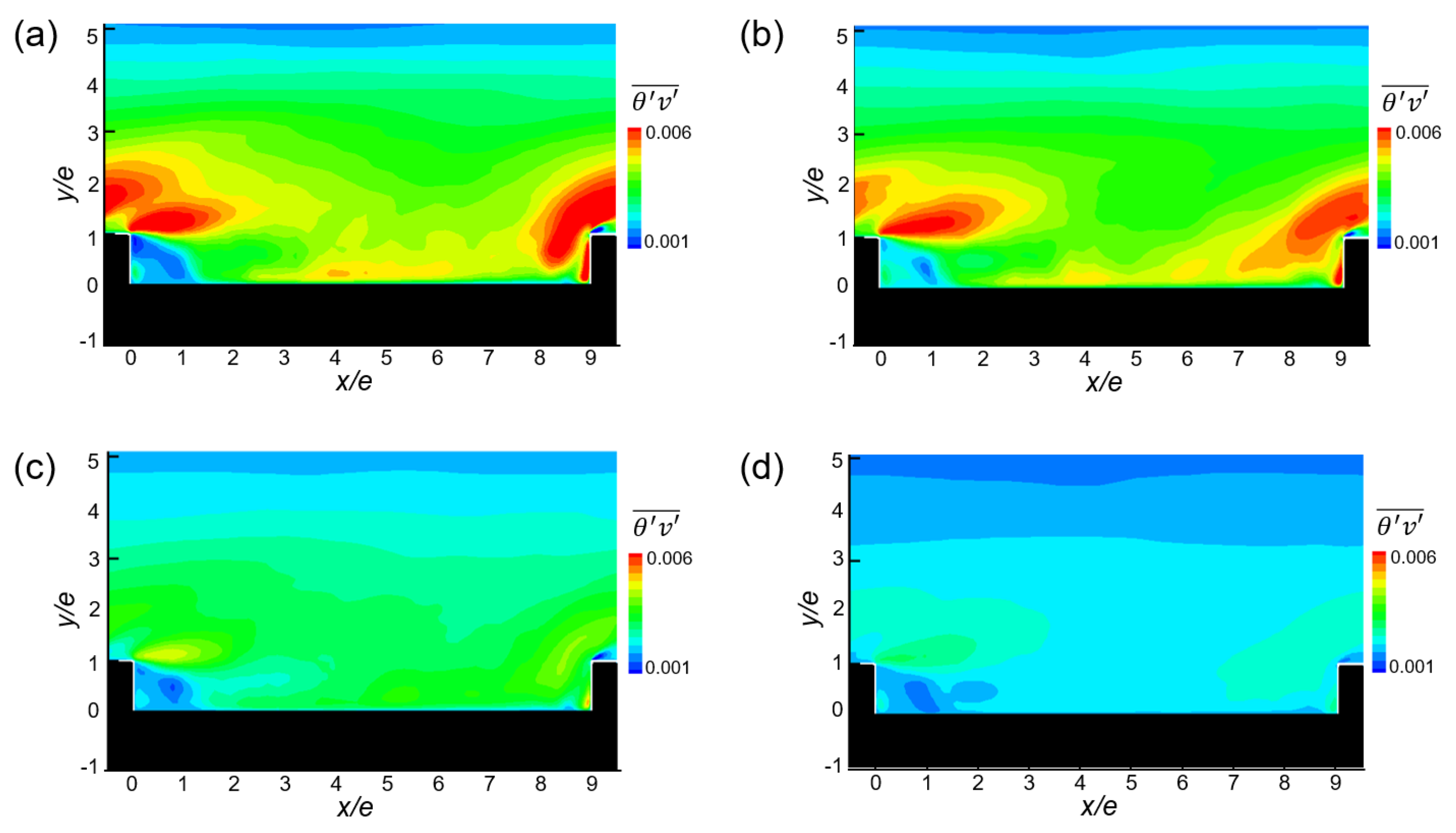
• For K* ≤ 10, the turbulent heat flux on the front face of the rib was concentrated at a corner, and the turbulent heat flux whose peak occurred near the channel wall disappeared.
• At K* = 100, the temperature fluctuation at the upstream edge of the rib reached 2%, and at K* = 1, the temperature fluctuation in the solid region was at a level similar to that in the fluid region.
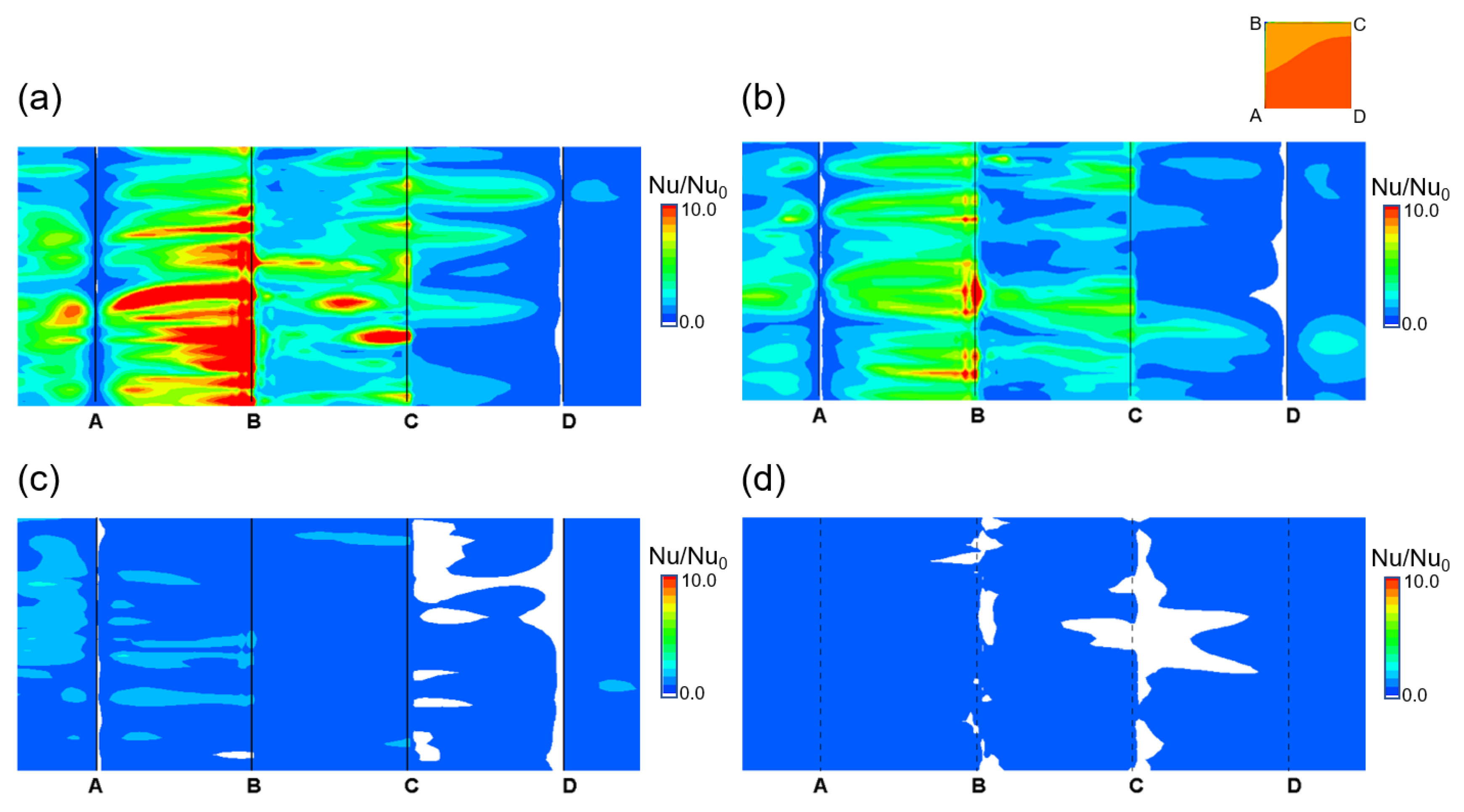
• Below K* = 100, heat transfer enhancement was significantly reduced by conduction. Up to K* = 100, the rib promoted heat transfer, but below K* = 10, it did not promote heat transfer.
• Compared with the thermal resistance of the solid and fluid for the CHT of the ribbed channel, the Biot number that was defined on the basis of the thickness of the channel wall appropriately represented the heat transfer characteristics. In other words, for K* = 100 or higher, the Biot number at the channel wall was considerably smaller than 0.1, but at K* = 1, it was considerably larger than 1, which was consistent with the thermal performance of the rib.

References

1. Srinivasan, V.; Simon, T.W.; Goldstein, R.J. Synopsis. In Heat Transfer in Gas Turbine Systems; The New York Academy of Science: New York, NY, USA, 2001; pp. 1–10. [Google Scholar]
2. Han, J.C. Fundamental Gas Turbine Heat Transfer. ASME J. Therm. Sci. Eng. Appl. 2013, 5, 021007. [Google Scholar] [CrossRef]
3. Han, J.C.; Park, J.S. Developing Heat Transfer in Rectangular Channels with Rib Turbulators. Int. J. Heat Mass Transf. 1988, 31, 183–195. [Google Scholar] [CrossRef]
4. Park, J.S.; Han, J.C.; Huang, S.; Ou, S.; Boyle, R.J. Heat Transfer Performance Comparisons of Five Different Rectangular Channels with Parallel Angled Ribs. Int. J. Heat Mass Transf. 1992, 35, 2891–2903. [Google Scholar] [CrossRef]
5. Ruck, S.; Arbeiter, F. Detached Eddy Simulation of Turbulent Flow and Heat Transfer in Cooling Channels Roughened by Variously Shaped Ribs on One Wall. Int. J. Heat Mass Transf. 2018, 118, 388–401. [Google Scholar] [CrossRef]
6. Liou, T.M.; Hwang, J.J. Effect of Ridge Shapes on Turbulent Heat Transfer and Friction in a Rectangular Channel. Int. J. Heat Mass Transf. 1993, 36, 931–940. [Google Scholar] [CrossRef]
7. Han, J.C.; Huh, M. Recent Studies in Turbine Blade Internal Cooling. Heat Transf. Res. 2010, 41, 803–828. [Google Scholar]
8. Kim, H.M.; Kim, K.Y. Design Optimization of Rib-Roughened Channel to Enhance Turbulent Heat Transfer. Int. J. Heat Mass Transf. 2004, 47, 5159–5168. [Google Scholar] [CrossRef]
9. Taslim, M.E.; Wadsworth, C.M. An Experimental Investigation of the Rib Surface-Averaged Heat Transfer Coefficient in a Rib-Roughened Square Passage. ASME J. Turbomach. 1997, 119, 381–389. [Google Scholar] [CrossRef]
10. Coletti, F.; Scialanga, M.; Arts, T. Experimental Investigation of Conjugate Heat Transfer in a Rib-Roughened Trailing Edge Channel with Corssing Jets. ASME J. Turbomach. 2012, 134, 041016. [Google Scholar] [CrossRef]
11. Ju, Y.; Feng, Y.; Zhang, C. Conjugate Heat Transfer Simulation and Entropy Generation Analysis of Gas Turbine Blades. ASME J. Eng. Gas Turbine Power 2021, 143, 081012. [Google Scholar] [CrossRef]
12. Yusefi, A.; Nejat, A.; Sabour, H. Ribbed Channel Heat Transfer Enhancement of an Internally Cooled Turbine Vane Using Cooling Conjugate Heat Transfer Simulation. Therm. Sci. Eng. Progress 2020, 19, 100641. [Google Scholar] [CrossRef]
13. Iaccarino, G.; Ooi, A.; Durbin, P.A.; Behnia, M. Conjugate Heat Transfer Predictions in Two-dimensional Ribbed Passages. Int. J. Heat Fluid Flow 2002, 23, 340–345. [Google Scholar] [CrossRef]
14. Cukurel, B.; Arts, T.; Selcan, C. Conjugate Heat Transfer Characterization in Cooling Channels. J. Therm. Sci. 2012, 21, 286–294. [Google Scholar] [CrossRef]
15. Cukurel, B.; Arts, T. Local Heat Transfer Dependency on Thermal Boundary Condition in Ribbed Cooling Channel Geometries. ASME J. Heat Transf. 2013, 135, 101001. [Google Scholar] [CrossRef]
16. Ooi, A.; Iaccarino, G.; Durbin, P.A.; Behnia, M. Reynolds Averaged Simulation of Flow and Heat Transfer in Ribbed Ducts. Int. J. Heat Fluid Flow 2002, 23, 750–757. [Google Scholar] [CrossRef]
17. Duchaine, F.; Gicquel, L.; Grosnickel, T.; Koupper, C. Large-Eddy Simulation of the Flow Developing in Static and Rotating Ribbed Channels. ASME J. Turbomach. 2020, 142, 041003. [Google Scholar] [CrossRef]
18. Ahn, J.; Choi, H.; Lee, J.S. Large Eddy Simulation of Flow and Heat Transfer in a Channel Roughened by Square or Semicircle Ribs. ASME J. Turbomach. 2005, 127, 263–269. [Google Scholar] [CrossRef]
19. Ahn, J.; Choi, H.; Lee, J.S. Large Eddy Simulation of Flow and Heat Transfer in a Rotating Ribbed Channel. Int. J. Heat Mass Transf. 2007, 50, 4937–4947. [Google Scholar] [CrossRef]
20. Scholl, S.; Verstraete, T.; Duchaine, F.; Gicquel, L. Influence of the Thermal Boundary Conditions on the Heat Transfer of a Rib-Roughened Cooling Channel Using LES. J. Power Energy 2015, 229, 498–507. [Google Scholar] [CrossRef]
21. Scholl, S.; Verstraete, T.; Duchaine, F.; Gicquel, L. Conjugate Heat Transfer of a Rib-Roughened Internal Turbine Blade Cooling Channel Using Large Eddy Simulation. Int. J. Heat Fluid Flow 2016, 61, 650–664. [Google Scholar] [CrossRef]
22. Fedrizzi, R.; Arts, T. Determination of the Conjugate Heat Transfer Performance of a Turbine Blade Cooling Channel. Quant. InfraRed Thermogr. J. 2004, 1, 71–88. [Google Scholar] [CrossRef]
23. Patil, S.; Tafti, D.K. Large-Eddy Simulation with Zonal Near Wall Treatment of Flow and Heat Transfer in a Ribbed Duct for the Internal Cooling of Turbine Blades. ASME J. Turbomach. 2013, 135, 031006. [Google Scholar] [CrossRef]
24. Oh, T.K.; Tafti, D.K.; Nagendra, K. Fully Coupled Large Eddy Simulation-Conjugate Heat Transfer Analysis of a Ribbed Cooling Passage Using the Immersed Boundary Method. ASME J. Turbomach. 2021, 143, 041012. [Google Scholar] [CrossRef]
25. Halila, E.E.; Lenahan, D.T.; Thomas, T.T. High Pressure Turbine Test Hardware Detailed Design Report; NASA CR-167955; NASA: Washington, DC, USA, 1982; pp. 18–68.
26. Romeyn, A. High Pressure Turbine Blade Fracture CFM56-3C1 Engine Test Cell, 7 July 2004; ATSB Transport Safety Investigation Report; Australian Transport Safety Bureau: Canberra, Australia, 2006; pp. 7–8.
27. Ahn, J.; Song, J.C.; Lee, J.S. Fully Coupled Large Eddy Simulation of Conjugate Heat Transfer in a Ribbed Channel with a 0.1 Blockage Ratio. Energies 2021, 14, 2096. [Google Scholar] [CrossRef]
28. Neuberger, H.; Hernandez, F.; Ruck, S.; Arbeiter, F.; Bonk, S.; Rieth, M.; Stratil, L.; Muller, O.; Volker, K.-U. Advances in Additive Manufacturing of Fusion Materials. Fusion Eng. Des. 2021, 167, 112309. [Google Scholar] [CrossRef]
29. Bang, M.; Kim, S.; Park, H.S.; Kim, T.; Rhee, D.-H.; Cho, H.H. Impingement/Effusion Cooling with a Hollow Cylinder Structure for Additive Manufacturing: Effect of Channel Gap Height. Int. J. Heat Mass Transf. 2021, 175, 121420. [Google Scholar] [CrossRef]
30. Ditaranto, M.; Heggset, T.; Berstad, D. Concept of Hydrogen Fired Gas Turbine Cycle with Exhaust Gas Recirculation: Assessment of Process Performance. Energy 2020, 192, 116646. [Google Scholar] [CrossRef]
31. Choi, H.; Moin, P. Effects of the Computational Time Step on Numerical Solutions on Turbulent Flow. J. Comp. Phys. 1994, 113, 1–4. [Google Scholar] [CrossRef]
32. Kim, J.; Kim, D.; Choi, H. An Immersed Boundary Finite Volume Method for Simulations of Flow in Complex Geometries. J. Comp. Phys. 2001, 171, 132–150. [Google Scholar] [CrossRef]
33. Kim, J.; Choi, H. An Immersed Boundary Finite Volume Method for Simulation of Heat Transfer in Complex Geometries. KSME Int. J. 2004, 18, 1026–1035. [Google Scholar] [CrossRef]
34. Song, J.C.; Ahn, J.; Lee, J.S. An Immersed-Boundary Method for Conjugate Heat Transfer Analysis. J. Mech. Sci. Technol. 2017, 31, 2287–2294. [Google Scholar] [CrossRef]
35. Tafti, D.K. Evaluating the Role of Subgrid Stress Modeling in a Ribbed Duct for the Internal Cooling of Turbine Blades. Int. J. Heat Fluid Flow 2005, 26, 92–104. [Google Scholar] [CrossRef]
36. Patankar, S.V.; Liu, C.H.; Sparrow, E.M. Fully Developed Flow and Heat Transfer in Ducts Having Streamwise-Periodic Variations of Cross-Sectional Area. ASME J. Heat Transf. 1977, 99, 180–186. [Google Scholar] [CrossRef]
37. Germano, M.; Piomelli, P.; Moin, P.; Cabot, W.H. A Dynamic Sub-grid Scale Eddy Viscosity Model. Phys. Fluids 1991, A3, 1760–1765. [Google Scholar] [CrossRef] [Green Version]
38. Lilly, D.K. A Proposed Modification of the Germano Sub-grid Scale Closure Model. Phys. Fluids 1992, A4, 633–635. [Google Scholar] [CrossRef]
39. Kong, H.; Choi, H.; Lee, J.S. Dissimilarity Between the Velocity and Temperature Fields in a Perturbed Turbulent Thermal Boundary Layer. Phys. Fluids 2001, 13, 1466–1479. [Google Scholar] [CrossRef]
40. Casarsa, L.; Arts, T. Experimental Investigation of the Aerothermal Performance of a High Blockage Rib-Roughened Cooling Channel. ASME J. Turbomach. 2005, 127, 580–588. [Google Scholar] [CrossRef]
41. Incropera, F.P.; Dewitt, D.P.; Bergman, T.L.; Lavine, A.S. Principles of Heat and Mass Transfer, 1st ed.; Wiley: Hoboken, NJ, USA, 2017; pp. 153–158. [Google Scholar]
42. Ramachandran, S.G.; Shih, T.I.-P. Biot Number Analogy for Design of Experiments in Turbine Cooling. ASME J. Turbomach. 2015, 137, 061002. [Google Scholar] [CrossRef] [Green Version]
43. Jung, E.Y.; Chung, H.; Choi, S.M.; Woo, T.K.; Cho, H.H. Conjugate Heat Transfer on Full-coverage Film Cooling with Array Jet Impingement with Various Biot numbers. Exp. Therm. Fluid Sci. 2017, 83, 1–8. [Google Scholar] [CrossRef]
Figure 1. Computational domain and grid system: (a) schematic diagram of the internal cooling passage; (b) the computational domain; and (c) the grid system.
Energies 14 05698 g001
Figure 2. Time-averaged flow and thermal fields for the isothermal wall: (a) comparison of time-averaged streamlines with particle image velocimetry measurement data of Casarsa et al. [40], (b) the time-averaged temperature field, and (c) the Nusselt number ratio on the channel wall between ribs.
Energies 14 05698 g002
Figure 3. Time-averaged thermal fields: (a) K* = 566.26, (b) K* = 100.00, (c) K* = 10.00, and (d) K* = 1.00.
Energies 14 05698 g003
Figure 4. Heat flux vectors inside the solid wall: (a) K* = 566.26, (b) K* = 100.00, (c) K* = 10.00, and (d) K* = 1.00.
Energies 14 05698 g004
Figure 5. Local temperature distribution at the solid–fluid interface: (a) the temperature along the interface between the ribs and (b) the temperature on the rib.
Energies 14 05698 g005
Figure 6. Effect of thermal resistance on local convective heat transfer along the solid–fluid interface: (a) heat transfer along the interface between the ribs and (b) heat transfer on the rib.
Energies 14 05698 g006
Figure 7. Turbulent heat flux θ v ¯ contours for (a) K* = 566.26, (b) K* = 100.00, (c) K* = 10.00, and (d) K* = 1.00.
Energies 14 05698 g007
Figure 8. Temperature fluctuations (θrms) for (a) K* = 566.26, (b) K* = 100.00, (c) K* = 10.00, and (d) K* = 1.00.
Energies 14 05698 g008
Figure 9. Instantaneous thermal fields near the rib for (a) K* = 566.26, (b) K* = 100.00, (c) K* = 10.00, and (d) K* = 1.00.
Energies 14 05698 g009
Figure 10. Instantaneous local heat transfer: (a) K* = 566.26; (b) K* = 100.0; (c) K* = 10.0; and (d) K* = 1.0.
Energies 14 05698 g010
Figure 11. Thermal performance: (a) fin performance of the rib and (b) the total heat transfer rate.
Energies 14 05698 g011
Figure 12. Local Biot number variations: (a) on the channel wall and (b) on the rib.
Energies 14 05698 g012