A Two-Parameter Model for Water-Lubricated Pipeline Transportation of Unconventional Crudes

Abstract

Water-lubricated flow technology is an environmentally friendly and economically beneficial means of transporting unconventional viscous crudes. The current research was initiated to investigate an engineering model suitable to estimate the frictional pressure losses in water-lubricated pipelines as a function of design/operating parameters such as flow rates, water content, pipe size, and liquid properties. The available models were reviewed and critically assessed for this purpose. As the reliability of the existing models was not found to be satisfactory, a new two-parameter model was developed based on a phenomenological analysis of the dataset available in the open literature. The experimental conditions for these data included pipe sizes and oil viscosities in the ranges of 25–260 mm and 1220–26,500 mPa·s, respectively. A similar range of water equivalent Reynolds numbers corresponding to the investigated flow conditions was 10³–10⁶. The predictions of the new model agreed well with the experimental results. The respective values of the coefficient of determination (R²) and the root mean square error (RMSE) were 0.90 and 0.46. The current model is more refined, easy-to-use, and adaptable compared to other existing models.

1. Introduction

One of the most challenging aspects in the process value chain of unconventional oils is transporting the extracted oils economically to a central processing facility from different remote production sites [1,2]. The conventional methods of transportation such as dilution, heating, or emulsion usually require reducing the effective viscosity to bring down the frictional pressure losses in the pipeline to an acceptable limit. An alternative means of transporting unconventional oils is the lubricated pipe flow (LPF). The more viscous oil is separated from the pipe wall with less viscous water by forming an annular flow pattern while flowing through a pipeline [3,4,5]. This flow system does not require any chemical-intensive expensive process for reducing the oil viscosity. The frictional pressure losses for the LPF were found to be comparable to that of transporting only water under similar process conditions. This flow technology has a proven capacity of significantly reducing the pump power for transporting unconventional viscous oils.

The LPF systems can be classified into three categories [2,6]:

(1)

core annular flow (CAF);

(2)

self-lubricated flow (SLF); and

(3)

water-assisted flow (WAF).

The CAF is an idealized concept of LPF. It refers to the formation of a viscous oil core continuously surrounded by a water annulus throughout the pipe, inhibiting the formation of a fouling oil layer on the pipe wall. Most of its reported applications have been in lab-scale pipelines under rigorously controlled process conditions to avoid fouling the wall with the viscous oil, whereas SLF and WAF refer to the types of LPF that are found in its industrial- and/or pilot-scale applications. The SLF is the pipeline transportation of bitumen froth with the application of LPF technology. Additional water is not required for SLF, as a froth typically contains bitumen, water, and sediments with volumetric concentrations of 60%, 30%, and 10%, respectively. The oil-rich core is exposed to the pipe wall at times causing wall-fouling in a SLF pipeline. This phenomenon renders the water lubrication a discontinuous function of pipe length. In the WAF, the frequency of the oil core touching pipe-wall is less frequent and the annular flow regime is more stable compared to SLF. Adding 20 to 30 vol% of water is necessary to produce the WAF regime, which involves varying degrees of wall-fouling as the viscous core may intermittently contact the pipe wall. It is possible to minimize the contact frequency and produce continuous water-assisted flow in practice by controlling the flow conditions.

The benefits of LPF have been appreciated ever since a CAF-based study was published by Russel and Charles [7]. Numerous further studies have been published to date. A fraction of these investigations addressed the difficult task of modeling the frictional pressure losses in different water-lubricated pipelines. Previously proposed models can be grouped into two categories [6,8,9]:

• single-fluid models;
• and two-fluid models.

An engineering approach was used in the single-fluid models for the prediction of pressure gradients by characterizing the multiphase flow in a water-lubricated pipeline with a single-phase flow of a hypothetical fluid. The corresponding Fanning friction factor (f) was regarded to have a power–law relationship with an equivalent Reynolds number (Re), f = K/Reⁿ, where K and n are constants. Examples of such models include Arney et al. [1], Rodriguez et al. [5], and Joseph et al. [10]. The hypothetical fluid for these models was either water or its properties, which correlated to the properties of the lubricated oil and the lubricating water. On the other hand, the two-fluid models were typically proposed for the idealized CAF in a smooth pipe made of glass, Plexiglass, or Perspex. The two-fluid models implement a mechanistic approach for the modeling and attempt to take into consideration the actual mechanism of friction losses in a CAF pipeline (see, e.g., [4,11,12,13,14,15]). However, this kind of model does not apply to SLF and WAF.

The industrial applications of LPF have had limited success in transporting non-conventional oils. The main constraint was the unavailability of a model that could provide accurate and reliable predictions for friction losses. A dependable and easy-to-use model is necessary to facilitate the efficient application of this flow technology. The most prominent of the existing models were assessed in this study. The current selection included the notable models proposed by Arney et al. [1], McKibben et al. [3], Rodriguez et al. [5], Joseph et al. [10], and Shi et al. [16]. The respective performances of these models were analyzed based on a set of experimental data collected from the literature [6,17]. Both the accuracy and reliability of the predictions of these models were found to be unsatisfactory. Consequently, a simpler, adaptable, and easy-to-use model was developed based on a phenomenological analysis for the frictional pressure losses in a WAF system. The efficacy of the current model was examined statistically by comparing its predictions to that of the previous models.

2. Materials and Methods

2.1. Experimental Data

Three independent datasets published in the literature were used for the current study [6,17]. The experiments were conducted in two high-quality research facilities: (1) Pipe Flow Technology Center, Saskatchewan Research Council (SRC), Saskatoon, SK, Canada; and (2) Process Systems Engineering Laboratory, Cranfield University (CU), Cranfield, UK. The experimental setup in SRC consisted of several recirculating pipelines made of stainless steel (SS). On the other hand, the experimental setup in CU was designed as a “once-through” flow line constructed with clear poly-vinyl chloride (PVC) material, Perspex. The experimental data are summarized below in

Table 1. Summary of the experimental conditions.

Data Source	Pipe Construction Material	Pipe Diameter (mm)	Average Velocity (m/s)	Oil Viscosity (mPa·s)	Water Viscosity (mPa·s)	Water Fraction (-)
[6]	SS	103.3 264.8	1.0 1.5 2.0	1220 1300 1400 16,600 26,500	0.67 0.72 0.89	0.17–0.43
[17]	PVC	26	0.19–1.728	3300 5600	1.27 1.00	0.30–0.79

.

2.2. Modeling Approach

2.2.1. Phenomenological Analysis

The ideal CAF is non-existent in any full-scale pipeline as it requires the entire pipe wall to remain water-wet during oil transport. The actual application of CAF or a fully developed WAF flow regime in a pipeline can be characterized by the following conditions:

• separation of the oil-rich core from the pipe wall by a thin water annulus;
• high viscosity and, therefore, negligible shear in the core;
• laminar or plug flow condition of the core;
• turbulent water annulus subjected to high shear;
• sporadic contacts between the wavy oil core and the pipe wall, thus forming a durable oil film on the pipe wall known as wall-fouling;
• entrapment of the turbulent water annulus between the stationary wall-fouling layer and the high-speed oil core; and
• turbulent water annulus resulting in an unusual roughness on the wall-fouling layer that further intensifies the shear in the annulus.

That is, WAF refers to the water-lubricated flow condition in which the pipe wall is coated with the viscous oil being transported through the pipeline. The frictional shear that ensues in such a complex multiphase flow system indeed has significant contributions from the turbulent water annulus, the laminar oil core, and the stationary wall-fouling layer characterized by an atypical surface roughness [8,15,18]. A phenomenological assessment was implemented in the current study to consider these contributing factors while modeling the WAF friction losses.

The pressure loss (ΔP/L) is known to be directly related to the wall shear stress (${\tau }_w$), Fanning friction coefficient (f), the internal diameter of the pipe (D), average fluid velocity (V), and fluid density (ρ) for the steady flow of an incompressible fluid in a pipeline as follows:

$$\frac{∆P}{L}=\frac{4{\tau }_w}{D}=f\frac{2V^2\rho }{D}$$

(1)

Based on Equation (1), an equivalent friction coefficient (f_waf) was defined for the WAF with the following equation:

$$f_{waf}={\left(\frac{∆P}{L}\right)}_{waf}\frac{D}{2V^2{\rho }_w}$$

(2)

Additionally, two pairs of equivalent Reynolds number (Re) and corresponding friction factors (f) were adapted as follows:

$$R{e}_w=\frac{DV{\rho }_w}{{\mu }_w}$$

(3)

$$f_w=\frac{0.079}{R{e}_w^{0.25}}$$

(4)

$$R{e}_o=\frac{DV{\rho }_o}{{\mu }_o}$$

(5)

$$f_o=\frac{16}{R{e}_o}$$

(6)

In Equations (3)–(6), Re_w is the water equivalent Re; Re_o is the oil equivalent Re; f_w is the water equivalent f; f_o is the oil equivalent f; ρ_w is the water density; ρ_o is the oil density; μ_w is the water viscosity; and μ_o is the oil viscosity. Equation (4) is Blasius law, while Equation (6) represents the f-Re correlation for laminar flow. Similar correlations have been used by previous researchers [1,3,5,10,16].

The magnitude of WAF friction losses is in between the similar energy consumptions for the single-phase transportations of heavy crude oil and water under comparable flow conditions [1,2,3,4,5,6,7,8,9,10,11,12,13,14,15,16,17,18,19]. This observation is illustrated in Figure 1, where values of three equivalent friction coefficients (f_waf, f_o, and f_w) are plotted against two equivalent Reynolds numbers (Re_w and Re_o). It is evident from the figure that f_waf can be expressed as a function of f_o, f_w, Re_w, and Re_o. The parameter f_waf includes both f_w and a fraction of f_o, as $f_{waf}=f_w+x{f}_o$. The fractional component x is a non-linear function of Re_w and Re_o. Based on this observation, we propose the following correlation:

$$f_{waf}=f_w+R{e}_o^{n}R{e}_w^k{f}_o=0.079R{e}_w{}^{-0.25}+16R{e}_o{}^{\left(n-1\right)}R{e}_w{}^k$$

(7)

where n and k are the coefficients that should be regressed based on a dataset.

2.2.2. Data Regression

The WAF data were divided into two sets based on the construction material of the pipelines: (1) SS data [6] and (2) PVC data [17]. Each dataset was divided further into two subsets: (1) modeling data and (2) test data. A total of 75% of the data was used for modeling while the remaining 25% was used for testing. The values of (n, k) were tuned based on the modeling dataset, and the test dataset was used to evaluate the model performance. The details of the data apportioning are summarized in

Table 2. Classification of data for regression.

Pipe Construction Material	Subset	Number of Data Points (%)	Pipe Diameter (mm)	Average Velocity (m/s)	Oil Viscosity (mPa·s)	Water Fraction (-)
SS	Modeling	36 (77%)	103.3 264.8	1.0 1.5 2.0	1300 1400 26,500	0.17–0.43
	Test	11 (23%)	103.3	1.0 1.5 2.0	1220 16,600	0.24–0.42
PVC	Modeling	21 (72%)	26	0.188–1.719	5600	0.24–0.79
	Test	8 (28%)	26	0.264–1.728	3300	0.19–0.68

.

The curve fitting toolbox version 3.5.11 available in MATLAB R2020A was used for the regression. The tool uses the method of least squares for fitting the data based on the Trust–Region algorithm, which minimizes the sum squared value of the residuals, $r_i$ (i.e., the difference between the observed value of the response), $f_{waf,i}$, and the corresponding fitted value, ${\widehat{f}}_{waf,i}$ [20]. The sum of the squares of the errors is given by the following equation:

$$L={\displaystyle \sum }_{i=1}^N{r}_i^2={\displaystyle \sum }_{i=1}^N{\left(f_{waf,i}-{\widehat{f}}_{waf,i}\right)}^2$$

(8)

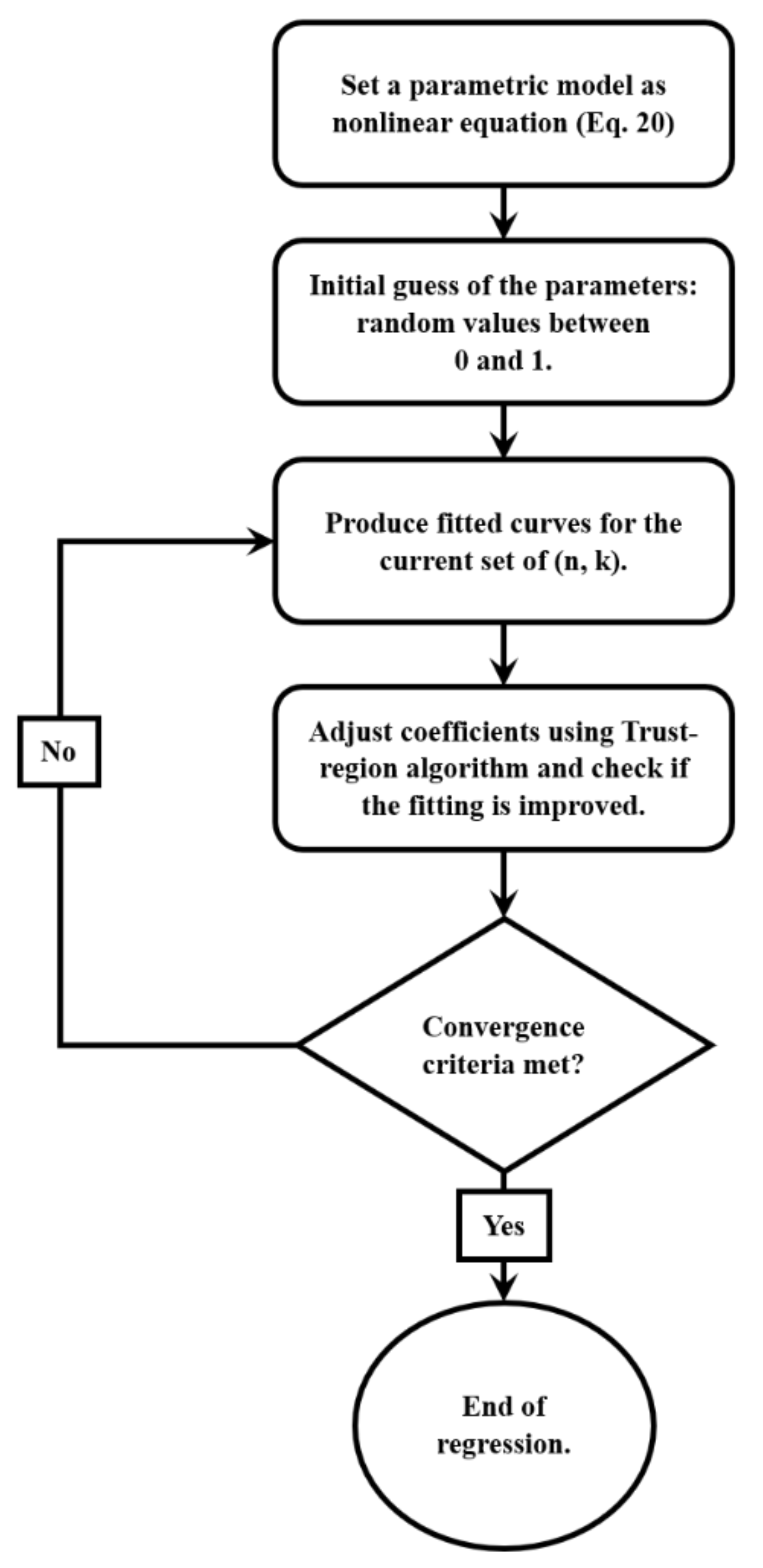
where N is the number of modeling data points used for the regression. An iterative approach presented in Figure 2 was necessary to fit the nonlinear model (Equation (7)). The iteration started with an initial guess to produce a fitted curve. The coefficients were then repeatedly adjusted until the convergence criteria were satisfied.

3. Results

3.1. Regression Output

The outcome of the current regression analysis (i.e., the optimum values of model co-efficient) were n = 0.4805 and k = 0.6196. Based on these values, Equation (7) can be rewritten as:

$$f_{waf}=0.079R{e}_w{}^{-0.25}+16R{e}_w{}^{0.6196}R{e}_o{}^{-0.5195}$$

(9)

Equation (9) represents the proposed model of the current study. It should be used in conjunction with Equation (2) to estimate the frictional pressure losses in a WAF pipeline.

3.2. Model Output

The performance of the current model is demonstrated in Figure 3. The experimental and predicted values of f_waf are presented against Re_w in this figure for the SS and PVC datasets separately. The current WAF model can predict both the trend and the magnitude of the friction factor within an acceptable error limit. The predicting accuracies for the modeling and test datasets are comparable, which proves its robustness.

4. Discussion

4.1. Performance of Existing Models

The current study was initiated with the aim to ascertain the best model for WAF pressure losses. Efforts were undertaken to develop a new model as the existing models failed to produce satisfactory predictions. In this regard, the predicting performance of the current model is discussed in comparison to the outcomes of the existing models.

4.1.1. Arney et al.’s Model

Arney et al. [1] developed a single fluid model based on a comprehensive CAF database. The material of construction for the lab-scale experimental pipeline was pragmatically selected as glass, which is hydrophilic and oleophobic. A glass pipe is known to be hydrodynamically smooth. The model is presented with Equations (10)–(14).

$$\frac{\mathsf{\Delta }P}{L}=f\frac{2{\rho }_c{V}^2}{D}$$

(10)

$$f=\frac{0.079}{R{e}_a{}^{0.25}},\hspace{1em}R{e}_a>4000$$

(11)

$$R{e}_a=\frac{{\rho }_{c}DV}{{\mu }_w}$$

(12)

$${\rho }_c=H_w{\rho }_w+\left(1-H_w\right){\rho }_o$$

(13)

$$H_w=C_w\left[1+0.35\left(1-C_w\right)\right]$$

(14)

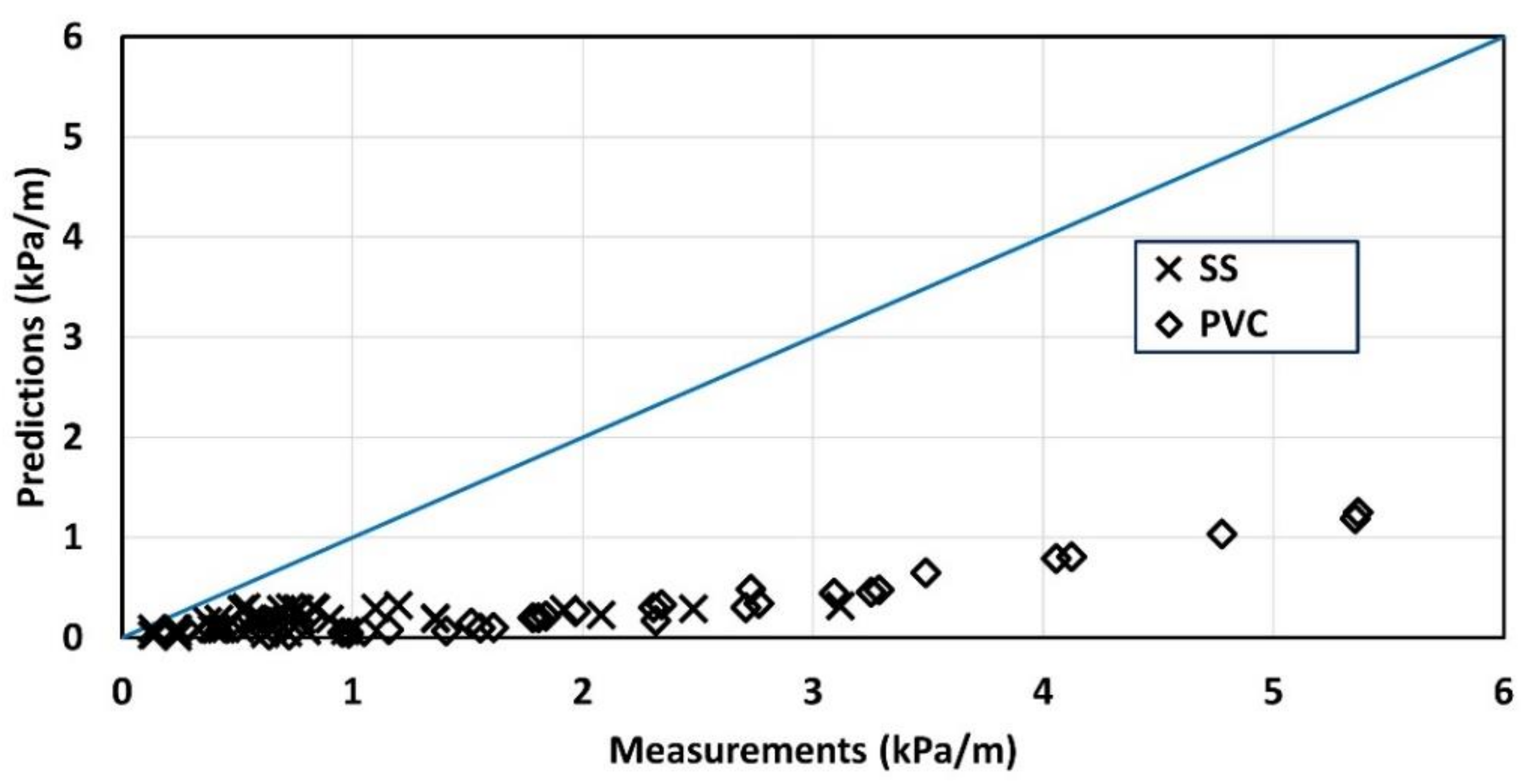
In Equations (10)–(14), ρ_c is the density of a model-specific hypothetical fluid; Re_a is an equivalent Re; H_w is the water hold-up; and C_w is the input water fraction. This CAF model was applied to the current WAF dataset to test its performance in predicting CWAF pressure losses. The results are presented in Figure 4. As shown in the figure, Arney et al. significantly underpredicted the experimental measurements. This is because it cannot address the issue of wall fouling, which is present in a WAF pipeline and increases the hydrodynamic roughness significantly.

4.1.2. Joseph et al.’s Model

Joseph et al. [10] studied the self-lubricated pipeline transportation of bitumen froth. The high internal shear released a part of the water inside the froth, resulting in a lubricating layer and forming an intermittent CAF regime with a noticeable layer of bitumen fouling the pipe wall. Based on the lab-scale and pilot-scale experiments, a single fluid model was proposed. The semi-empirical model used a Blasius-type correlation that relates the friction factor to a water equivalent Reynolds number as follows:

$$f=\frac{0.079K_j}{R{e}_w^{0.25}}$$

(15)

$$\frac{\mathsf{\Delta }P}{L}=f\frac{2{\rho }_w{V}^2}{D}$$

(16)

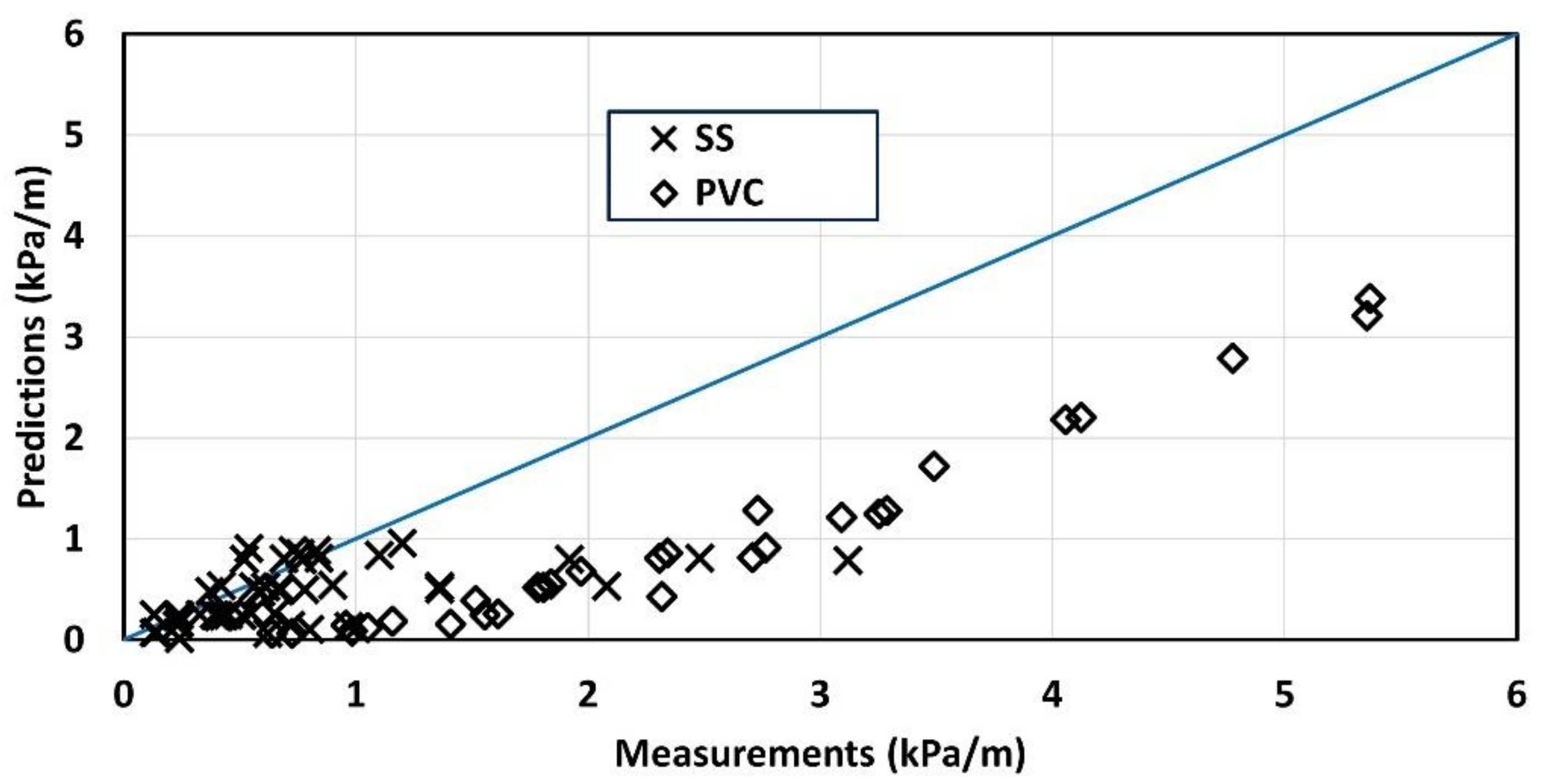
where K_j = 23 (at 35–47 °C) and 16 (at 49–58 °C). The constant $K_j$ was considered a function of temperature only. The effect of water fraction on $K_j$ was not considered. For a set of flow conditions, the value of friction loss predicted using this model was usually 15–40 times higher than the similar energy consumption for transporting only water under identical flow conditions. That is, the energy requirement for SLF was much higher. This is primarily due to the significant wall-fouling as well as the high frequency of contact between the core and the pipe wall. This is why this model significantly overpredicted the actual values of pressure losses as it was applied to the current WAF dataset (Figure 5).

4.1.3. Rodriguez et al.’s Model

Rodriguez et al. [5] developed a semi-mechanistic model using both lab- and pilot-scale data for the horizontal CAF of heavy oils. The effects of annular flow regimes, kinetics, buoyancy, and wall conditions including fouling were considered for the modeling. PVC pipes were used in the laboratory, while a steel pipe was used in the field. By analyzing the data in a semi-mechanistic approach, a friction loss model was proposed as follows:

$$f=\frac{\mathrm{b}}{4}{\left(\frac{{\mathsf{\rho }}_{\mathrm{w}}\mathrm{VD}}{{\mathsf{\mu }}_{\mathrm{w}}}\right)}^{-\mathrm{n}}{\left[1-\left(1-\frac{{\mathsf{\rho }}_{\mathrm{o}}}{{\mathsf{\rho }}_{\mathrm{w}}}\right)\frac{1}{1+\mathrm{s}\frac{{\mathrm{U}}_{\mathrm{w}}}{\mathrm{V}}}\right]}^{1-\mathrm{n}}{\left(1-\frac{1}{1+\mathrm{s}\frac{{\mathrm{U}}_{\mathrm{w}}}{\mathrm{V}}}\right)}^{-\mathrm{n}}{\left[1+\left(\mathrm{s}-1\right)\frac{1}{1+\mathrm{s}\frac{{\mathrm{U}}_{\mathrm{w}}}{\mathrm{V}}}\right]}^{\mathrm{n}-2}$$

(17)

where $\mathrm{b}$ and n are the empirical constants; s is the slip ratio; and ${\mathrm{U}}_{\mathrm{w}}$ is the water superficial velocity. The following values of $\mathrm{b}$ and n were determined empirically with an actual dataset:

n = 0.25

b = 0.16 (less fouled pipe wall)

= 0.76 (highly fouled pipe wall)

The slip ratio (s) was correlated to oil hold up (H_o) and superficial velocities (U_o and U_w) with non-linear relationships as follows:

$$U_o\left(1-H_o\right)-1.17U_w{H}_o-0.02H_o^{1.79}=0$$

(18)

$$s=1.17+\frac{0.05}{V_w}{H}_o^{0.8}$$

(19)

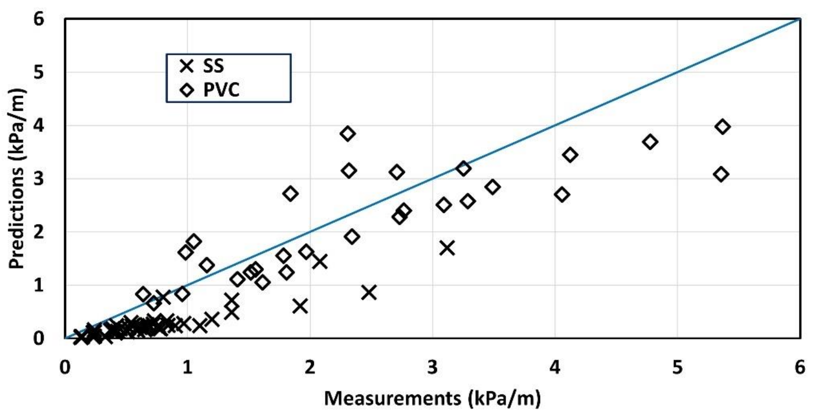
An iterative solution using Equations (18) and (19) is required for s, as it is implicitly correlated to H_o. Even though the application of this correlation is more complicated and time-consuming compared to Arney et al. and Joseph et al., its performance was better in predicting the WAF pressure losses to some extent (Figure 6). This is because the dataset used to formulate Rodriguez et al. was developed based on the flow conditions that involved both smooth and fouled pipe walls. Nevertheless, its performance cannot be considered satisfactory as it failed to predict either the trend or the magnitude of the current WAF data.

4.1.4. McKibben et al.’s Model

McKibben et al. [3] proposed a phenomenological model based on decade-long research dedicated to the WAF phenomena. The flow tests were conducted using SS pipes. More than 400 WAF datasets were analyzed to propose the following correlation:

$$f=15{\left(Fr\right)}^{-0.5}{f}_{\mathrm{w}}^{1.3}{f}_{\mathrm{o}}^{0.32}{\mathrm{C}}_{\mathrm{w}}^{-1.2}$$

(20)

$$Fr=\frac{\mathrm{V}}{\sqrt{\mathrm{gD}}}$$

(21)

where Fr is the Froude number and g is the gravitational acceleration. The water equivalent friction factor, f_w, and the oil equivalent friction factor, f_o, were defined earlier with Equations (4) and (6), respectively. This model is supposed to consider the effects of buoyancy, inertia, oil viscosity, water fraction, and wall-fouling. As applied to the current WAF dataset (Figure 7), it provided better performance compared to the models discussed earlier. However, it involved over predictions and a high degree of uncertainty.

4.1.5. Shi et al.’s Model

Shi et al. [16] studied the pressure gradients in the water-lubricated flow of viscous oil. During the flow tests, a CAF regime with wall-fouling (i.e., a WAF regime) was identified as the dominating flow category for the following ranges of superficial velocities:

U_o: 0.04–0.56 m/s; U_w: 0.03–1 m/s

An empirical model for friction losses was developed using the data acquired from the experimental study. A simplified form of the model is presented as follows:

$$f=\frac{b}{4}{\left(\frac{DV\left(\raisebox{1ex}{$U_o{\rho }_o$}\!\left/ \!\raisebox{-1ex}{$V$}\right.+\left(1-\raisebox{1ex}{$U_o$}\!\left/ \!\raisebox{-1ex}{$V$}\right.\right){\rho }_w\right)}{\frac{{\mu }_w}{1-\raisebox{1ex}{$U_o$}\!\left/ \!\raisebox{-1ex}{$V$}\right.}}\right)}^{-n}$$

(22)

This is a modified version of a CAF model proposed earlier by Bannwart [21]. The values of the model constants (b, n) were (0.066, 0.047) for the Bannwart model. The magnitude of these constants had to be augmented by orders of magnitude to fit with the WAF data. For Shi et al., the values of (b, n) were (6228, 1.1). Although it provided better results compared to other models (Figure 8), its performance cannot be considered satisfactory due to the considerable uncertainty and dispersion in the predictions. It should also be noted that a part of the current dataset, namely, the PVC data, was used to develop this model.

4.2. Classification of the Existing Models

The performances of the models discussed earlier were evaluated further on a single platform based on two dimensionless parameters, f_waf and Re_w. The values of f_waf were determined using the experimental measurements and the predicted values of ΔP/L (Equation (2)). The existing models were divided further into two categories based on their respective origins and predicting capabilities as follows.

4.2.1. Non-WAF Models

Arney et al. [1], Joseph et al. [10], and Rodriguez et al. [5] did not propose the respective models for any WAF systems. As mentioned previously, these models were developed for the following usages:

Arney et al.: idealized CAF with continuous lubrication and without any wall-fouling;

Joseph et al.: SLF with a high degree of wall-fouling and intermittent water lubrication; and

Rodriguez et al.: non-ideal CAF with an unknown degree of wall-fouling.

The hydrodynamic effect of the wall-fouling layer was not appropriately addressed in these pioneering studies. Hence, these models failed to reproduce the trend in WAF friction losses. Arney et al. significantly underestimated the experimental results, while the same results were over-predicted by Joseph et al. It is interesting to note that Rodriguez et al. could predict the data better than the CAF and SLF model. This is because it was developed for imperfect CAF pipelines where wall-fouling could not be resisted even after undertaking efforts to do so.

4.2.2. Water-Assisted Flow Models

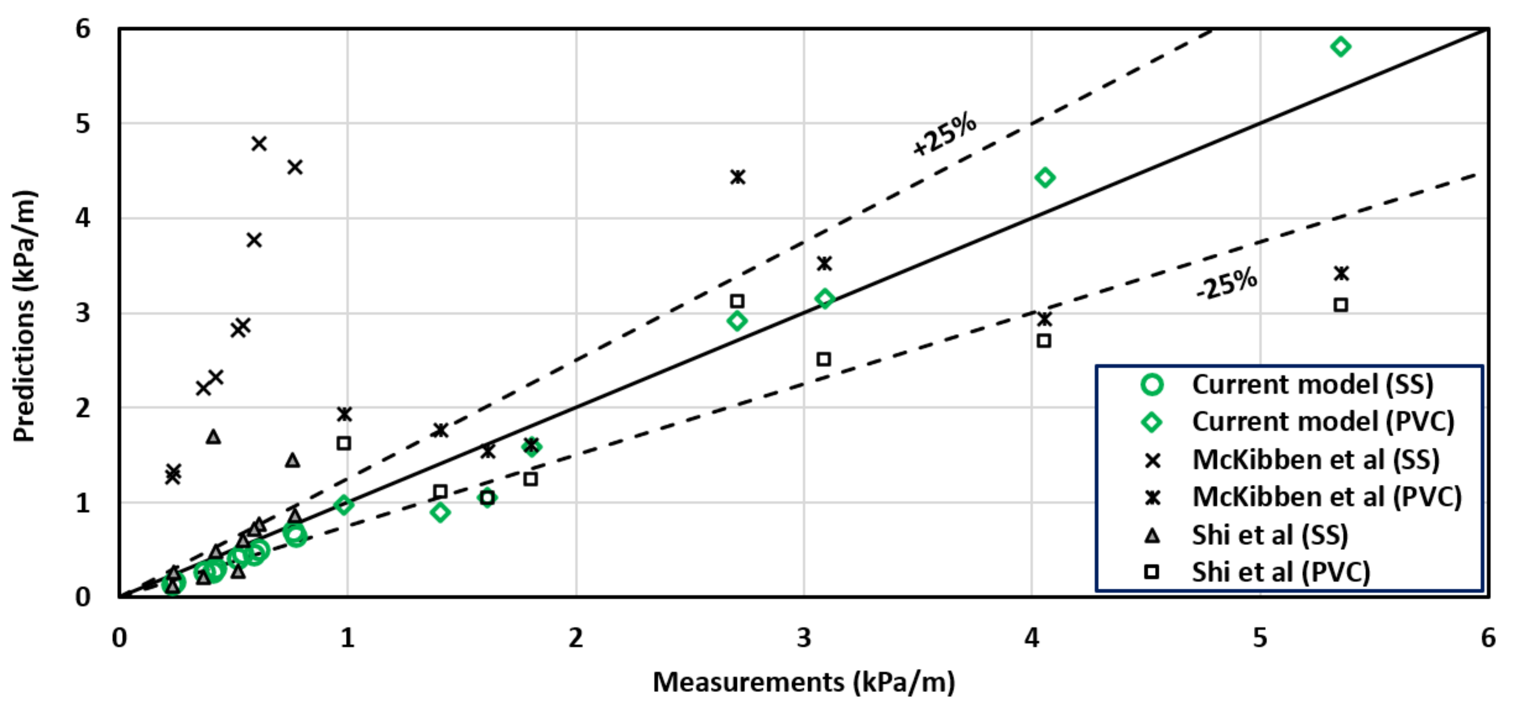
The models of Shi et al. and McKibben et al. were developed for WAF systems. Unlike non-WAF models, both models can replicate the trend in experimental data appreciably well (Figure 9).

Although Shi et al. can estimate the magnitude of the data produced using a PVC pipe (CU data), its performance is poor for steel pipes (SRC data). This type of disagreement underscores its empirical nature. McKibben et al., on the other hand, produces better results for both SRC and CU data. This model was developed based on a phenomenological approach, instead of an absolute empirical inference. The contribution of wall fouling to the WAF frictional shear was considered by covering a wide variety of lab- and pilot-scale flow conditions. Nevertheless, its predictions involve notable deviations from the actual measurements. The most significant shortcoming of McKibben et al. is its higher number of coefficients (Equation (20)) compared to other similar models. It is a five-parameter model and not adaptable to the flow conditions beyond its boundary limit as that would necessitate tuning five coefficients. Moreover, both WAF models are incapable of addressing the non-linearity of the data.

4.3. Performance of the Current Model

The prediction accuracy of the current model in comparison to other WAF models is presented in Figure 9. It endorses a direct comparison of the WAF models based on the test dataset. Most of the data points could be predicted by the current model within an error margin of ±25%, which is noticeably less than that of the other models. Moreover, it produces the least dispersion or variability of the predictions and can address the non-linearity of the data.

4.4. Statistical Analysis

Acceptance of a model heavily depends on its validation. Instead of relying only on the visual endorsement or a single statistical measurement, the current model was validated by exploiting a selected number of statistical parameters [22,23,24,25,26,27,28,29,30,31]. Only the test datasets were used for the present statistical analysis that allowed us to compare the performances of the WAF models objectively.

4.4.1. Coefficient of Determination

The coefficient of determination illustrates the goodness of the data fitting quantitatively. The corresponding R² expresses the predicting strength of a model and its capability to reduce the variation of the regression. It was defined as follows [22]:

$$R^2=1-\frac{{{\displaystyle \sum }}_{i=1}^N{\left[{\left(\raisebox{1ex}{$∆P$}\!\left/ \!\raisebox{-1ex}{$L$}\right.\right)}_{pred,i}-{\left(\raisebox{1ex}{$∆P$}\!\left/ \!\raisebox{-1ex}{$L$}\right.\right)}_{exp,i}\right]}^2}{{{\displaystyle \sum }}_{i=1}^N{\left[{\left(\raisebox{1ex}{$∆P$}\!\left/ \!\raisebox{-1ex}{$L$}\right.\right)}_{pred,i}-\overline{{\left(\raisebox{1ex}{$∆P$}\!\left/ \!\raisebox{-1ex}{$L$}\right.\right)}_{exp,i}}\right]}^2}$$

(23)

where N is the total number of data points; ${\left(\raisebox{1ex}{$∆P$}\!\left/ \!\raisebox{-1ex}{$L$}\right.\right)}_{pred,i}$ is the predicted values of pressure gradient or friction loss; ${\left(\raisebox{1ex}{$∆P$}\!\left/ \!\raisebox{-1ex}{$L$}\right.\right)}_{exp,i}$ is the experimentally measured values of pressure loss; and $\overline{{\left(\raisebox{1ex}{$∆P$}\!\left/ \!\raisebox{-1ex}{$L$}\right.\right)}_{exp,i}}$ is the arithmetic average of measured pressure gradients. The magnitude of R² varies within a range of 0 to 1. R² = 1 indicates that 100% of the variation of the predicted pressure gradients can be attributed to the experimental values, while R² = 0 shows the absolute incompetence of the model in explaining any variability of the data [23].

Respective values of R² for the WAF models are presented in

Table 3. Coefficient of determination and root mean square error of water-assisted flow models.

Models	R2	RMSE
McKibben et al.	0.15	2.21
Shi et al.	−0.11	0.80
Current model	0.85	0.45

. The proposed model performed appreciably better than other models as it yielded the highest value of $R^2$ (R² = 0.85). That is, it could significantly minimize the differences between the measured and predicted values of the WAF pressure gradients. The values of R² for other models were either negative or less than 0.2, which means that these are not applicable to predict the trend and magnitude of the data with acceptable precision.

4.4.2. Root Mean Square Error

The root-mean-square error (RMSE), also called the residual standard deviation, is the standard deviation of the residual values [24]. It measures how scattered the residuals are and quantifies the concentration of the data around the prediction line. RMSE = 0 signifies the absence of errors in the regression (i.e., all measured values to coincide with the predictions). A similar condition is also represented by $R^2$ = 1. The RMSE was calculated using the following relation [22]:

$$RMSE=\sqrt{\frac{1}{N}{\displaystyle \sum }_{i=1}^N{\left[{\left(\raisebox{1ex}{$∆P$}\!\left/ \!\raisebox{-1ex}{$L$}\right.\right)}_{exp,i}-{\left(\raisebox{1ex}{$∆P$}\!\left/ \!\raisebox{-1ex}{$L$}\right.\right)}_{pred,i}\right]}^2}$$

(24)

The values of RMSEs are reported in Table 3. The lowest value of RMSE was for the current model. Higher RMSEs for other models underscore their inherent incapability of yielding reliable predictions.

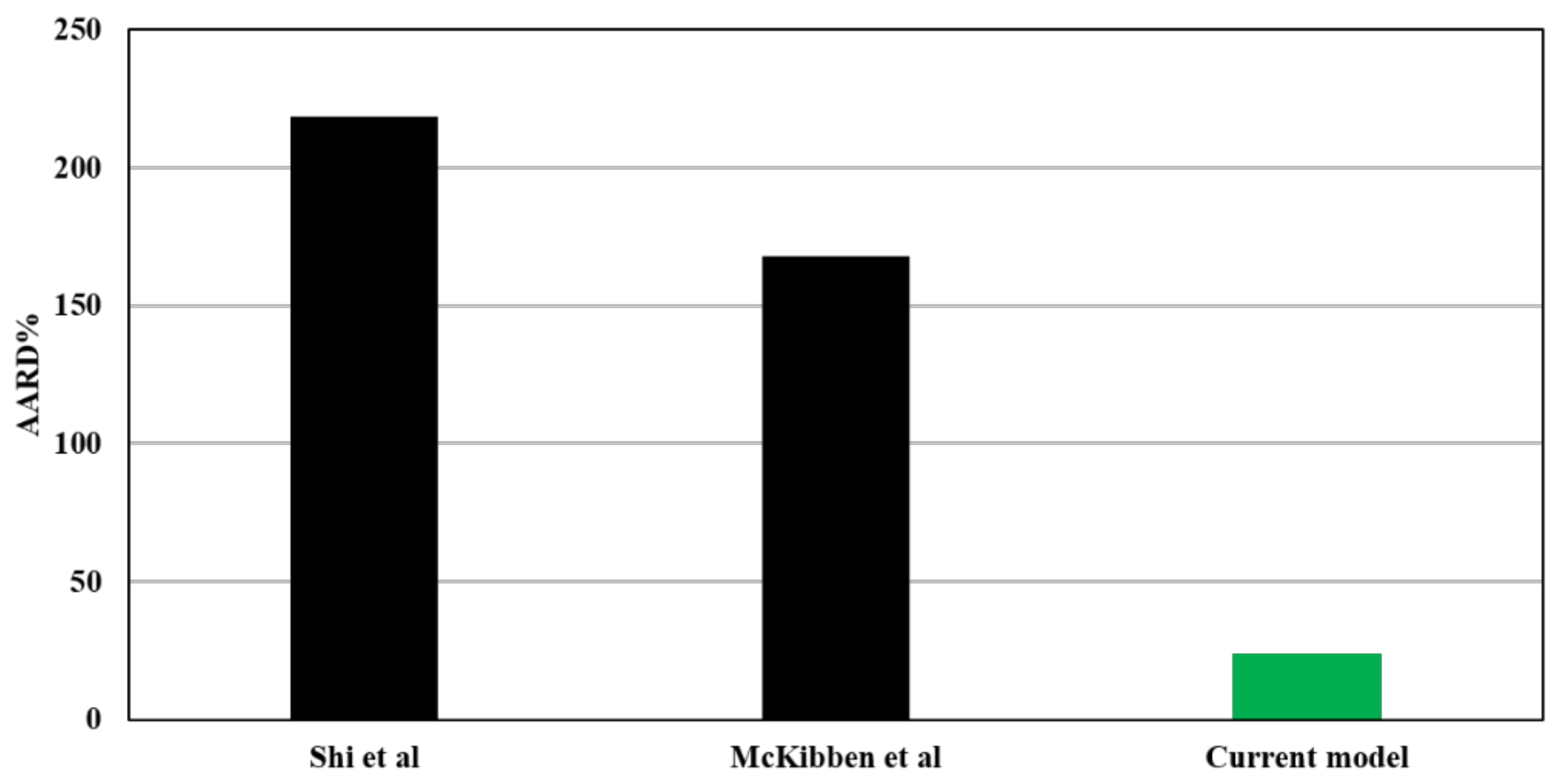
4.4.3. Average Absolute Relative Deviation

The average absolute relative deviation (AARD) measures the average magnitude of the difference between the predictions and the measurements. It provides a quantitative idea of the extent of the dispersion and the relative amount of deviation [25]. The following equation was used to calculate AARD [22]:

$$AARD=\frac{1}{N}{\displaystyle \sum }_{i=1}^N\frac{\left|{\left(\raisebox{1ex}{$∆P$}\!\left/ \!\raisebox{-1ex}{$L$}\right.\right)}_{exp,i}-{\left(\raisebox{1ex}{$∆P$}\!\left/ \!\raisebox{-1ex}{$L$}\right.\right)}_{pred,i}\right|}{{\left(\raisebox{1ex}{$∆P$}\!\left/ \!\raisebox{-1ex}{$L$}\right.\right)}_{exp,i}}$$

(25)

Figure 10 shows the comparative values of AARD for different models. The proposed model produced the lowest magnitude of AARD (i.e., its predictions were least dispersed).

5. Conclusions

The purpose of the current study was to find a reliable model that can be used to design WAF pipelines. As part of the research, the most relevant models available in the literature were reviewed and analyzed using independent datasets. The performance of these models could not be considered as satisfactory, as some of these models were found to be complicated and most of those were susceptible to process conditions. The predicting capabilities of the previous models were not satisfactory. A new two-parameter model was developed with a phenomenological analysis of the data. The current study can be summarized as follows:

(1)

Two separate sets of pressure gradient data were collected from the literature. Stainless steel and PVC pipelines were used to generate the data. The experimental pipe sizes varied within a broad range of 25 mm to 265 mm. The oil viscosity and the water fraction were also changed over wide ranges of 1.22–26.5 Pa.s and 0.1–0.79, respectively.

(2)

The proposed model could be implemented for the SS and PVC datasets. It provided satisfactory predictions for both datasets, which proves its robustness and adaptability. The model estimates were within ±25% of the experimental measurements.

(3)

The R² was significantly higher, while the RMSE and the AARD were considerably lower for the current model compared to other models.

The model proposed in this study was, thus, validated to be adaptable and capable of producing reliable predictions. It was developed by applying a simple regression algorithm. Efforts are underway to apply artificial intelligence-based data regression techniques such as machine learning algorithms.

References

1. Arney, M.S.; Bai, R.; Guevara, E.; Joseph, D.D.; Liu, K. Friction factor and holdup studies for lubricated pipelining-I. Experiments and correlations. Int. J. Multiph. Flow 1993, 19, 1061–1076. [Google Scholar] [CrossRef]
2. Hart, A. A review of technologies for transporting heavy crude oil and bitumen via pipelines. J. Pet. Explor. Prod. Technol. 2014, 4, 327–336. [Google Scholar] [CrossRef] [Green Version]
3. McKibben, M.; Sanders, S.; Gillies, R. A new method for predicting friction losses and solids deposition during the water-assisted pipeline transport of heavy oils and co-produced sand. In Proceedings of the SPE Heavy Oil Conference-Canada, Calgary, AB, Canada, 11–13 June 2013. [Google Scholar] [CrossRef]
4. Ho, W.S.; Li, N.N. Core-annular flow of liquid membrane emulsion. AIChE J. 1994, 40, 1961–1968. [Google Scholar] [CrossRef]
5. Rodriguez, O.M.H.; Bannwart, A.C.; de Carvalho, C.H.M. Pressure loss in core-annular flow: Modeling, experimental investigation and full-scale experiments. J. Pet. Sci. Eng. 2009, 65, 67–75. [Google Scholar] [CrossRef]
6. Rushd, M.M.A.S. A New Approach to Model Friction Losses in the Water-Assisted Pipeline Transportation of Heavy Oil and Bitumen. Ph.D. Thesis, University of Alberta, Edmonton, AB, Canada, 2016. [Google Scholar] [CrossRef]
7. Russell, T.W.F.; Charles, M.E. The effect of the less viscous liquid in the laminar flow of two immiscible liquids. Can. J. Chem. Eng. 1959, 37, 18–24. [Google Scholar] [CrossRef]
8. Rushd, S.; McKibben, M.; Sanders, R.S. A new approach to model friction losses in the water-assisted pipeline transportation of heavy oil and bitumen. Can. J. Chem. Eng. 2019, 97, 2347–2358. [Google Scholar] [CrossRef]
9. Rushd, S.; Sultan, R.A.; Mahmud, S. Modeling Friction Losses in the Water-Assisted Pipeline Transportation of Heavy Oil. In Processing of Heavy Crude Oils: Challenges and Opportunities; Gounder, R.M., Ed.; IntechOpen: London, UK, 2019. [Google Scholar] [CrossRef] [Green Version]
10. Joseph, D.D.; Bai, R.; Mata, C.; Sury, K.; Grant, C. Self-lubricated transport of bitumen froth. J. Fluid Mech. 1999, 386, 127–148. [Google Scholar] [CrossRef] [Green Version]
11. Oliemans, R.V.A.; Ooms, G. Core-Annular Flow of Oil and Water through a Pipeline. In Multiphase Science and Technology; Hewitt, G.F., Delhaye, J.M., Zuber, N., Eds.; Springer: Berlin/Heidelberg, Germany, 1986. [Google Scholar] [CrossRef]
12. Crivelaro, K.C.; Damacena, Y.T.; Andrade, T.H.; Lima, A.G.; Farias Neto, S.R. Numerical simulation of heavy oil flows in pipes using the core-annular flow technique. WIT Trans. Eng. Sci. 2009, 63, 193–203. [Google Scholar] [CrossRef] [Green Version]
13. de Andrade, T.H.F.; Crivelaro, K.C.O.; de Farias Neto, S.R.; de Lima, A.G.B. Numerical Study of Heavy Oil Flow on Horizontal Pipe Lubricated by Water. In Materials with Complex Behaviour II; Öchsner, A., da Silva, L., Altenbach, H., Eds.; Springer: Berlin/Heidelberg, Germany, 2012. [Google Scholar] [CrossRef]
14. Kaushik, V.V.; Ghosh, S.; Das, G.; Das, P.K. CFD simulation of core annular flow through sudden contraction and expansion. J. Petrol. Sci. Eng. 2012, 86, 153–164. [Google Scholar] [CrossRef]
15. Shi, J.; Gourma, M.; Yeung, H. CFD simulation of horizontal oil-water flow with matched density and medium viscosity ratio in different flow regimes. J. Petrol. Sci. Eng. 2017, 151, 373–383. [Google Scholar] [CrossRef] [Green Version]
16. Shi, J.; Lao, L.; Yeung, H. Water-lubricated transport of high-viscosity oil in horizontal pipes: The water holdup and pressure gradient. Int. J. Multiph. Flow 2017, 96, 70–85. [Google Scholar] [CrossRef] [Green Version]
17. Shi, J. A study on High-Viscosity Oil-Water Two-Phase Flow in Horizontal Pipes. Ph.D. Thesis, Cranfield University, Cranfield, UK, 2015. [Google Scholar]
18. Rushd, S.; Sanders, R.S. A parametric study of the hydrodynamic roughness produced by a wall coating layer of heavy oil. Pet. Sci. 2017, 14, 155–166. [Google Scholar] [CrossRef] [PubMed] [Green Version]
19. McKibben, M.J.; Gillies, R.G.; Shook, C.A. Predicting pressure gradients in heavy oil-water pipelines. Can. J. Chem. Eng. 2000, 78, 752–756. [Google Scholar] [CrossRef]
20. Branch, M.A.; Coleman, T.F.; Li, Y. Subspace, interior, and conjugate gradient method for large-scale bound-constrained minimization problems. SIAM J. Sci. Comput. 1999, 21, 1–23. [Google Scholar] [CrossRef]
21. Bannwart, A.C. Modeling aspects of oil–water core–annular flows. J. Pet. Sci. Eng. 2001, 32, 127–143. [Google Scholar] [CrossRef]
22. Halali, M.A.; Azari, V.; Arabloo, M.; Mohammadi, A.H.; Bahadori, A. Application of a radial basis function neural network to estimate pressure gradient in water–oil pipelines. J. Taiwan Inst. Chem. Eng. 2016, 58, 189–202. [Google Scholar] [CrossRef]
23. Rudolf, J.F.; William, J.W.; Ping, S. Regression Analysis: Statistical Modeling of a Response Variable, 2nd ed.; Elsevier: Amsterdam, The Netherlands, 2006; p. 459. [Google Scholar]
24. Chai, T.; Draxler, R.R. Root mean square error (RMSE) or mean absolute error (MAE)?-Arguments against avoiding RMSE in the literature. Geosci. Model Dev. 2014, 7, 1247–1250. [Google Scholar] [CrossRef] [Green Version]
25. Blaikie, C.N. Descriptive Analysis—Univariate Looking for Characteristics. In Analyzing Quantitative Data from Description to Explanation; Sage Publications: London, UK, 2003; pp. 47–88. [Google Scholar] [CrossRef] [Green Version]
26. Alizadehdakhel, A.; Rahimi, M.; Sanjari, J.; Alsairafi, A.A. CFD and artificial neural network modeling of two-phase flow pressure drop. Int. Commun. Heat Mass Transf. 2009, 36, 850–856. [Google Scholar] [CrossRef]
27. Zabihi, R.; Mowla, D.; Karami, H.R. Artificial intelligence approach to predict drag reduction in crude oil pipelines. J. Pet. Sci. Eng. 2019, 178, 586–593. [Google Scholar] [CrossRef]
28. Boostani, M.; Karimi, H.; Azizi, S. Heat transfer to oil-water flow in horizontal and inclined pipes: Experimental investigation and ANN modeling. Int. J. Therm. Sci. 2017, 111, 340–350. [Google Scholar] [CrossRef]
29. Meeker, W.Q.; Hahn, G.J.; Escobar, L.A. Statistical Intervals: A Guide for Practitioners and Researchers; John Wiley & Sons: Hoboken, NJ, USA, 2017; pp. 23–36. [Google Scholar]
30. Bewick, V.; Cheek, L.; Ball, J. Statistics review 7: Correlation and Regression. Crit. Care 2003, 7, 451–459. [Google Scholar] [CrossRef] [PubMed] [Green Version]
31. Brahimi, T. Using Artificial Intelligence to Predict Wind Speed for Energy Application in Saudi Arabia. Energies 2019, 12, 4669. [Google Scholar] [CrossRef] [Green Version]
Figure 1. Comparative presentation of equivalent friction factor for the water-assisted flow of a 6450 mPa·s heavy crude in a 53 mm stainless steel pipeline [19] as a function of (a) Rew and (b) Reo.
Energies 14 05665 g001
Figure 2. A block diagram showing the regression procedure used to determine (n, k).
Energies 14 05665 g002
Figure 3. Predictions of the current model: (a) stainless steel dataset; (b) poly-vinyl chloride PVC dataset.
Energies 14 05665 g003
Figure 4. Performance of Arney et al. in predicting the pressure losses in water-assisted flow pipelines.
Energies 14 05665 g004
Figure 5. Performance of Joseph et al. in predicting the pressure losses in water-assisted flow pipelines.
Energies 14 05665 g005
Figure 6. Performance of Rodriguez et al. in predicting the pressure losses in water-assisted flow pipelines.
Energies 14 05665 g006
Figure 7. Performance of McKibben et al. in predicting the pressure losses in water-assisted flow pipelines.
Energies 14 05665 g007
Figure 8. Performance of Shi et al. in predicting the pressure losses in water-assisted flow pipelines.
Energies 14 05665 g008
Figure 9. Comparative presentation of the prediction accuracies of the water-assisted flow models for the test datasets.
Energies 14 05665 g009
Figure 10. Comparison of average absolute relative deviation (AARD%) values for water-assisted flow models.
Energies 14 05665 g010