Abstract
Harmonic resonances are part of the power quality (PQ) problems of electrified railways and have serious consequences for the continuity of service and integrity of components in terms of overvoltage stress. The interaction between traction power stations (TPSs) and trains that causes line resonances is briefly reviewed, showing the dependence on infrastructure conditions. The objective is monitoring of resonance conditions at the onboard pantograph interface, which is new with respect to the approaches proposed in the literature and is equally applicable to TPS terminals. Voltage and current spectra, and derived impedance and power spectra, are analyzed, proposing a compact and efficient method based on short-time Fourier transform that is suitable for real-time implementation, possibly with the hardware available onboard for energy metering and harmonic interference monitoring. The methods are tested by sweeping long recordings taken at some European railways, covering cases of longer and shorter supply sections, with a range of resonance frequencies of about one decade. They give insight into the spectral behavior of resonances, their dependency on position and change over time, and the criteria needed to recognize genuine infrastructure resonances from rolling stock emissions.
1. Introduction
Railways are being used worldwide as an efficient and effective transportation infrastructure for people and goods, both long distance and within an urban context. Peculiarly, the traction supply arrangement differs from three-phase industrial networks in several aspects: AC railways are single phase operated at the medium voltage (MV) level, they have a physical extension typical of a transmission network but separated into smaller sections for most AC railways, the traction line feeds power to distributed moving loads (the trains), and the interaction between traction power stations (TPSs) and trains causes a variety of power quality (PQ) phenomena that are relevant to internal operation and disturbance to third parties [1]. In particular, as mainly focused on by the EN 50388 standards [2,3] regarding the interaction between rolling stock and the supply traction line, harmonic distortion and, in general, conducted emissions may cause local disturbances to signaling and control devices as well as supply line distortion, instability, and overvoltages. The first have been subject to extensive research for PQ indexes and criteria [1], as well as compensation strategies and implementations [4,5,6,7,8]. The latter are the objectives of recent research aimed at defining the conditions for line instability, harmonic resonances, consequences in terms of excessive distortion, and insulation breakdown [9,10,11,12,13].
Supply traction lines of some tens of km or longer, with significant capacitive loading due to MV cables, transformers, and trains (with their own onboard devices), exhibit a wide range of resonance phenomena, occurring in the frequency interval of a hundred of Hz up to some kHz, depending on the supply arrangement and length [14]. Traction systems in use today are mostly operated at 25 kV 50/60 Hz and 15 kV 16.7 Hz with different supply schemes. The supply sections of the latter are much longer, with extensive earthing bringing the resonant frequency of the line in the lower part of the considered frequency range, namely one or a few hundred Hz. The 2 × 25 kV systems have shorter supply sections with resonances in the kHz range [15,16,17,18,19,20,21], according to recent investigations for a series of resonance incidents [1,9]. As shown in [9,22], in a real scenario the response of the line may be quite complex.
The behavior of the traction line impedance with fixed feeding points (the TPSs) and moving loads (the trains) was initially analyzed, among others, in [14], proposing simple one-dimensional models based on transmission-line theory and indicating the high-level conditions for line resonance, as recalled by [9]. Basically, a line resonance occurs when the inductive and capacitive reactance terms with opposite signs are nearly equal in amplitude and compensate, leading to extreme conditions of very small or very large terminal impedance, depending on whether such elements are series or parallel connected. As for elementary resonant circuits, series and parallel resonances lead to situations of current or voltage amplification at the resonant frequency.
A real system is a more complex and articulated combination of series and parallel connected elements. The overall traction line can be subdivided into different sub-circuits that are relevant to define and analyze propagation of harmonics and coupling onto a range of affected systems. The harmonics propagate along the pantograph and catenary system and along the return circuit, pertaining to the so-called hot and cold paths. The cold path is relevant for induced and conducted disturbance onto signaling and communication systems that share the track with the traction supply circuit; the studied circuit must include an accurate model of the return circuit, of common to differential signal transformation, and of local resonances. The hot path, conversely, concerns mainly the traction supply and overhead distribution system with an overall return along the return circuit and earth; the studied circuit is relevant for distortion shared by the TPSs and trains, and propagated back onto the high voltage feeding line and then into the public grid.
Resonances can occur between the elements interconnected by the long traction line over a broad frequency range, concretizing as low-frequency and high-frequency oscillations (identified as LFOs and HFOs, respectively). Recalling the EN 50388 standards [2,3] and the interpretation given in [9], it may be said that LFOs are related to system instability [23], mostly caused by delay and phase rotation along the line [24] and interaction of active controls onboard rolling stock, applying power factor compensation [25,26]. This led to the catastrophic blackout of the Swiss network in April 1995 (as reported in [25,27]) and significant research activity among the infrastructure owners, manufacturers, and scholars. A comprehensive list of incidents caused by network resonances is reported in [1] and a detailed list of those which occurred in China is reported in [9].
HFOs, along with causing overvoltages, are sometimes interpreted as a PQ problem, where network resonances are excited by the rolling stock harmonic emissions and by transient phenomena, such as the electric arc at pantograph [28]. Network resonances are of course subject to variability depending on loading and the relative position and the type of trains in the supply section, although the theory of the one-dimensional transmission line suggests that main resonances do not depend on train position [9,14]. Such slight variability, in particular for secondary resonances, was observed during tests carried out in a well-documented system, the test ring at Velim in Czechia, where the influence of train position every 500 m, including traction supply cables, was investigated [29]. The longer the traction supply section between two TPSs, the lower the main resonant frequency, as theoretically demonstrated in [14] and taken up and commented by [9].
The consequence of parallel resonances occurring in the hot path is an increase in the distortion injected back into the public grid and, most of all, line voltage amplification, with potentially catastrophic effects:
- excessive instantaneous voltage may trigger TPS overvoltage protections, possibly causing cascaded tripping and the collapse of a large portion of the railway’s electric network,
- overvoltage stress in terms of single or repeated overvoltages of varying intensity that may cause the failure of surge arresters, likely resulting in a short circuit through the failed unit and a sudden TPS out-of-service due to protection tripping.
Series resonances may also occur [15], where the propagation of distortion involves the TPS and the upstream network, resulting in an increased distortion injected into the public grid. Sainz et al. traced correspondences between these resonances and the zeros of the pantograph impedance Zp. In general, major series resonance should occur in the lower part of the HFO range, where the series resistance is lower and the risk of excitation by low-order harmonics is higher, and consequences are thus worse.
As HFOs are caused by the resonance of TPS and the line while accounting for distributed and lumped capacitance terms, and are excited by rolling stock emissions, two approaches may be identified for harmonic and resonance suppression: ground-based suppression and on-board suppression [9]. Among ground-based suppression techniques, use of passive and active filters installed at TPSs is the most common solution [30], although some network’s reconfigurations may also be considered in order to shift the resonance frequency and reduce the factor of merit. On-board suppression may be achieved by installing passive filters, which may be exposed to excessive stress when an entire line section with resonance excited by nearby trains occurs [9]. On-board suppression most often relies on the modification of the converter modulation, rather than a revolutionary change of topology [31].
Converter control can be initiated and adapted if continuous monitoring of the pantograph quantities and of incipient line resonances is provided. Similarly, critical situations and the necessity of suppression implementation for a given line may be assessed if pantograph quantities are available and evaluated. In fact, this work discusses practical conditions for detection of resonance conditions from a railway vehicle perspective, using information available at the pantograph electric interface. Other measurement techniques have been proposed in the past [9,30,32], using purposely developed equipment located at TPS. The focus here instead is on the observability of resonance phenomena from the pantograph interface, to provide a distributed monitoring system that can be, in principle, installed onboard all the trains of the network.
The work is structured as follows: Section 2 describes the quantities and conditions for resonance to occur; Section 3 goes into the details of the detection and interpretation of harmonic resonances; Section 4 reports the results obtained from measured data collected during test runs in Switzerland and France, thus covering both 16.7 Hz and 50 Hz traction supply systems.
2. Network Resonance
As shown in [9], the system may be analyzed by means of multiconductor transmission line (MTL) equations, representing the overall network as a meshed set of series and parallel connected branches, to which lumped circuits (such as the TPS and the train as well as auxiliary transformers, including the pole mounted step-down transformers considered in [16]) may be attached at nodes. Although often neglected, MV connecting cables between TPS and the traction line may give a significant additional capacitance, which can bring the “natural” resonance of the supply section to a lower frequency (see considerations on the relevance of such parameters for exact fitting of measured frequency response in [29]). Similarly, adding capacitance to the train, as for the roof’s HV cable joining the two pantographs or a separate capacitor for arcing emission reduction [28], reduces the resonance frequency.
For the analysis of the hot path there is in general no need of a detailed model of the conductors forming the return path (the “cold path”); conversely, studying track-connected signaling circuits requires attention to track balance and rail-to-rail and rail-to-earth parameters. The hot path is often studied using simplification of conductors at the same potential into equivalent conductors [33], as considered also in [9] (see refs no. 92 and 93 there). However, the accuracy of the simplification worsens with increasing frequency [33,34], so that while this approach may be used for load flow studies and electromechanical simulation, it could lead to errors when frequencies of one to some kHz are considered, as they are for HFOs.
Network resonances depend on the studied transfer function and may be different if considering different quantities:
- the TPS voltage to evaluate the occurrence of overvoltages and the impact of TPS equipment,
- the line current flowing through the TPS transformer, as a PQ phenomenon impacting on the feeding network upstream,
- the pantograph voltage as a measure of parallel resonance along the line and the chance of interfering with the operation of the onboard converters,
- the pantograph current providing direct information on the exchanged active and reactive power and disturbance to track signaling, if interpreted as a return current.
Considering, in particular, the effect of the additional capacitance provided by the high-voltage cables wayside and onboard, the local train-based measurement of line resonances becomes more relevant.
Focusing on the source of the distortion exciting the traction line resonances and on the available measurements from the locomotive (or electro-train), the impedance is modeled at the pantograph-line interface, as carried out in [9,14]. The simplified schematic is shown in Figure 1.
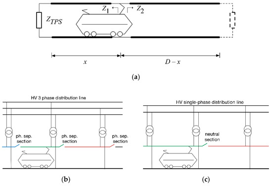
Figure 1.
(a) Simplified equivalent circuit for the AC traction line seen at the pantograph port; (b) single-side supply scheme typical of 25 kV 50/60 Hz systems; (c) portion of an interconnected network typical of 15 kV 16.7 Hz systems.
The frequency response of a railway line depends first of all on its length, and in particular on the length of the supply section, when this is electrically separated from the adjacent sections. The 50/60 Hz systems have the necessity of strict separation of each supply section, being derived from the national grid by loading alternatively two of the three phases (each supply section has thus a phase rotation of 120° electrical degrees); this is achieved by the phase separation sections, more commonly altogether named “neutral sections”. Conversely, 16.7 Hz systems have in several countries (such as Switzerland) a dedicated single-phase distribution and transmission network upstream, so that a phase separation is not, in principle, necessary. Then, mainly exigencies of network stability and continuity of service require the use of some neutral sections, more separated than for 50/60 Hz systems. To fix the ideas, the length for a 50/60 Hz high-speed line is in the order of 40 km, whereas for 16.7 Hz systems it may be in the order of a hundred km.
From the point of view of HFO modeling, this has two consequences:
- A longer supply section implies that HFOs begin in principle at a lower frequency, although a direct proportionality between length for the two systems is not correct, as there are differences in the traction conductors and per-unit-length parameters.
- The ideal equivalent circuit arrangement for 50/60 Hz and 16.7 Hz systems differs in that the former always has one TPS at one end of the line and the other end is left floating against the neutral section, whereas for the latter there may be configurations with more than one TPS with a piece of line terminated on a TPS at each end, without electrical separation. These two cases are shown below for completeness.
The impedance resulting from the parallel combination of the left and right sections at the pantograph connection point gives the following known expressions, having assumed a typical single-side supply scheme, as in 25 kV systems (see Figure 1a):
The resonance condition results from:
Now, in [9] a purely inductive ZTPS is assumed and the tanh( ) function is simplified with its own argument, so that (3) reduces to:
having indicated with C the total capacitance of the line. The first objection may be that the inductance of the line has disappeared, but neglecting the shunt conductance as sensible for the overhead conductors of the traction supply, the term in and in simplify in the fraction (small letters indicate per-unit-length parameters).
For a system without phase separation points and longer supply sections separated by some neutral sections, as in the case of 16.7 Hz railways (shown in Figure 1c), the two-terminal impedance condition at many locations are those of ZTPS at each side. This is a simplification that neglects the two adjacent line sections beyond the considered TPSs that are assumed to represent a low-impedance termination.
At resonance, inductive and capacitive terms compensate, leaving a line impedance with resistive behavior [35,36]. The resistive term should then be determined quite accurately, and the skin effect should be taken into account for a correct estimate of damping and height of the impedance peaks. Similarly, the depth of anti-resonance (or series resonance) points depends on the series resistance, chiefly influenced by skin effect in the traction supply conductors. For traction line conductors, skin effect is prominent in the running rails [37,38], whereas overhead conductors are not appreciably affected, being made of metals with negligible magnetic permeability in addition to their smaller cross section. Transformers at TPS and on-board can increase the overall line loss and may introduce some proximity effect within their windings; this explains the fact that stray inductance (that by definition represents the uncoupled magnetic field in air and is a linear term) is slightly frequency dependent.
3. Resonance Detection
Network impedance and resonance measurement methods may be broadly classified in active and passive methods, the former actively applying test signals to the network, whereas the latter listens passively to the accessible electrical quantities [39,40,41]. Active methods are invasive, necessitate precautions to interface the test signal generator to the high-voltage railway traction supply [9] and are more suited for ground installation, rather than onboard. Measuring line impedance and resonance effects without injecting a test signal, but exploiting the accessible electrical quantities at the pantograph interface, has the drawback instead of increased noise, incoherence between various spectral components of the same quantity, and a more jagged and noisy impedance curve.
The selected approach for onboard implementation is a passive method measuring electrical quantities at pantograph and mimicking an expert’s behavior when observing an ideal display that contains a set of signal characteristics extracted from the original input quantities. Such characteristics correspond to the spectrum components of the pantograph voltage and current, together with other derived quantities (impedance and power terms). Investigated criteria regard the abnormal increase in some spectrum components, together with their specific behavior vs. time. The approach considers the analogous behavior of adjacent spectrum components in order to discard isolated components, possibly caused by onboard power converters, that do not match the assumption of a limited factor of merit and broader resonance peaks.
3.1. Selected Pantograph Quantities and Basic Fourier Analysis
With the objective of detecting incipient resonances in real time using on-board instrumentation, as discussed in Section 2, the quantities that are accessible at the pantograph interface are Vp and Ip, the frequency domain spectra of the pantograph voltage and current, obtained from the corresponding vp and ip time waveforms. The same approach can then be transferred to the TPS, where the available quantities are the line voltage Vl and each feeder current If,k, or the total line current Il.
Spectra are calculated with a short-time Fourier transform (STFT) approach, with care to use P ≥ 2 periods of the fundamental f1 for demonstration purposes to set a frequency resolution df = f1/P that has the following advantages:
- it attenuates rapid transients lasting less than one cycle,
- it displays well even and odd harmonics with at least one intermediate bin between each of them; we should remember, however, that odd harmonics prevail and have a behavior coherent with the train’s operating conditions, so that they are even more separated and exempt from significant spectral leakage from the adjacent components,
- it allows the use of tapering windows with a broad main lobe (such as flat-top), as the resulting reduction in frequency resolution is less than a factor of 2 anyway with respect to the implicit rectangular window.
In any case, the signals can be analyzed with a percentage of overlap p ≥ 50%, ensuring a time resolution down to the fundamental period without hindering the desirable real-time response and frequency resolution.
3.2. Resonance Conditions
Resonance of an electrical circuit is defined as the situation at a given frequency where inductive and capacitive reactance in a loop are equal in magnitude and opposite in sign so that they cancel each other, resulting in an exchange of energy between the two, stored alternatively in the magnetic field of the inductive parts and the electric field of the capacitive parts. The resulting oscillation is internal to the loop and the externally visible effect is that of extremely small or large resistive impedance for series and parallel resonances, respectively.
A HFO condition occurs at the maxima of pantograph impedance Zp as a parallel resonance; the line voltage resonance then occurs if there corresponds a significant current excitation close to the identified resonance frequency. A series resonance occurs at the zeros of the same Zp, causing a maximization of the current flowing back down to the TPS, and possibly upstream. In both cases, the resistance of the return circuit due to the skin effect in the running rails [37,38] plays a major role and reduces the factor of merit, especially when observing the increase in minima and reduction in maxima of the Zp curve.
Practically speaking, with values of the factor of merit Q in the order of 10, the bandwidth δf around the ideal resonance frequency fr, which is proportional to 1/Q, so about 10%, will represent an interval with non-negligible width, bracketing more than one harmonic component, when fr is of the order of magnitude of one or more kHz. This is confirmed by the voltage spectra shown in [18,20,21] and discussed later in Section 4.
δf = fr / Q
The lower the Q factor, the lower the peak at resonance and the less relevant the effect of such resonance and the necessity to detect it.
At resonance (parallel or series one) the reactive components compensate and the net resulting impedance has a real value. This condition translates into the voltage Vh and current Ih phasors at the resonance frequency being in phase.
From a harmonic power flow point of view this is equivalent to a cancellation of the harmonic reactive power term Qh at the said resonance frequency, maximizing the harmonic active power fraction. Remember that the term “harmonic reactive power” results from the direct multiplication of voltage and current phasors at the same frequency, neglecting distortion power terms resulting from mixed multiplication of voltage and current phasors at different frequencies [35,36]. It is not meant by this that the active power term Ph is maximum overall, but its fraction taken with respect to the total harmonic apparent power Ah = √(Ph2+Qh2) (namely the harmonic displacement factor dh = Ph/Ah) is. This is clear as all low-order harmonics are characterized by large values of apparent power and consequently, in proportion, active power as well, as demonstrated in [42]. The use of dh allows a normalized weighting of the active power flow at all frequencies without problems of scale, with which resonance conditions may be characterized and identified.
What is also observed is that the harmonic power flow at the resonant frequency is prevalently active (theoretically only active power would flow in relation to circuit losses). As the analysis is carried out at the characteristic harmonics of the traction supply fundamental that might not coincide with the observed resonant frequency, the cancellation of the harmonic reactive power terms may be only approximate.
However, cancellation of reactive power at a given harmonic is a necessary, but not sufficient, condition for identification of network resonances, series or parallel. In fact, there are transient situations, as identified in the polar plots of the harmonic active and reactive power components in [42], for which the reactive power term may be temporarily very small with active power prevailing. This behavior was investigated in [43] to identify suitable PQ source indicators, focusing in particular on the sign and intensity of the active power indicator.
The harmonic active power Ph has thus proven itself as a valid indicator of power flow and behavior of harmonic power sources, as well as of resonance conditions, with a better discernibility than for voltage and current quantities alone. As the product of the two quantities, it has better scale properties than their quotient, i.e., the pantograph impedance Zp.
The transient conditions mentioned, in any case, last namely for a limited amount of time and are often related to the train’s operating conditions, whereas network resonances are more persistent and may depend only slightly on train position. Thus, an additional criterion to reject the vast majority of such transients is that the identified resonance condition last longer than the typical transient duration, that may be assumed to be some seconds, based on practice [42].
In addition, recalling the considerations on the factor of merit Q, a network resonance will affect several frequency bins at which there will be a significant increase in the harmonic power factor, whereas a loco emission is often limited to one or few harmonics.
From the definition of HFO it is understood also that a network parallel resonance as such should be accompanied by some amount of voltage amplification. Series resonances instead should be characterized by low voltage components and correspondingly current amplification.
3.3. Detection Criteria
Regarding criteria for detection, all harmonic components and the basic frequency resolution may be used, as well as grouped harmonics and a band-pass approach.
The most direct approach is based on detecting an excessive distortion of Vp that would cause the increase in the peak and rms values of the waveform. Alternatively, the attention may be focused on the peak and rms values of the waveform in an attempt to avoid the Fourier analysis. The peak value is nevertheless exposed to transients that would be detected as false positives; the rms value instead requires a calculation whose complexity is approximately that of a FFT implementation. In addition, the use of harmonic spectra allows the implementation of additional criteria, as the presence of adjacent harmonics and harmonic grouping.
Therefore, a time interval where some distortion threshold is exceeded is marked as a first candidate for resonance detection, although the excessive voltage distortion may be caused by an excess of current distortion due, e.g., to a particular operating point of the rolling stock power system. Confirmation comes from the corresponding assessment of current distortion at the same harmonics, verifying that it does not exceed a suitable threshold. This is equivalent to the verification of a sufficiently large Zp to justify the increased distortion observed in Vp, in turn not caused by an increase in Ip.
A set of rules is given identifying the criteria for the identification of resonance conditions, HFO, and their time behavior.
Rule 1: a resonance condition configures around the peaks of Zp, the local maxima of the network impedance curve at the pantograph interface; frequency bins satisfying such a condition form the set Hr,1 (set of indexes h satisfying rule 1).
Rule 2: HFO is triggered if the rolling stock has emissions exciting the resonance and if this is visible in the Vp spectrum, peaking around the resonance frequency.
Rule 3: an incipient HFO situation with an increase in a voltage component Vp,h* can be prevented, once distinguished from a momentary increase in a current component Ip,h* (e.g., caused by a transient operation of onboard converters), for which the ratio Zp = Vp/Ip is taken into account.
In general, the identification of the resonance is made on a semi-quantitative basis, where the detection of a fractional increase in Zp and Vp is sufficient (as it will be demonstrated in Section 5 with experimental data); the uncertainty requirement for the measurement of the pantograph quantities is thus not demanding and fits existing transducers and instrumentation already installed for monitoring purposes.
As observed in practice, converters’ emissions in the kHz range may be accompanied by a slight increase in Zp, due, for example, to the inductive behavior of the onboard transformer through which such emissions flow. However, such an increase is limited to a few spectral lines, so that it might be distinguished from a HFO due to the apparent larger Q factor. To make the interpretation of the Zp spectrum easier and less prone to errors, a robust check is carried out by combining the Zp spectrum with the distribution of dh values, resulting in the filtered impedance Z′p. A convenient threshold dthr = 0.9 was determined with some trial and error, with respect to the discernibility and interpretability of the resulting graphs, but also inspired from the often adopted value of 0.9 as a limit for the fundamental displacement factor (or power factor in general) in AC railways and distribution networks. Such threshold value, as commented below, may be slightly increased [36,42], but its physical meaning remains; it cannot be too close to unity as the frequency resolution limits the capability of capturing the ideal reactive power cancellation at resonance.
Rule 4: a HFO is confirmed if dh ≥ dthr (dthr = 0.9 is a convenient threshold, but other values, maybe slightly larger, are possible); frequency bins satisfying such condition form the set Hr,4 (set of indexes h satisfying rule 4).
The intersection of sets Hr,1 and Hr,4 indicates the frequency interval that satisfies both rules 1 and 4: Hr = Hr,1 ∩ Hr,4. This effectively removes many extraneous points and makes easier the interpretation of 2-D STFT spectrum of Z′p.
The confirmation of a HFO condition with parallel resonance comes from a local increase in voltage distortion components. To this aim, the Vp spectrum is scaled by normalizing it with respect to the fundamental value at the same time instant (), and for an exigency of scale, only harmonic values are displayed, discarding the fundamental and the larger low-frequency components.
A further confirmation, as anticipated at the end of Section 3.2, is the time duration for which the same hypothetical resonance condition (holding all rules 1 to 4 so far) persists for a preset time interval.
Rule 5: a HFO is confirmed if the bins in the set Hr defined above remain in the set for a sufficient time duration set to TH,min.
From , it is possible to evaluate the overall distortion as total harmonic distortion (THD), just by taking the rooted sum of squares:
This approach is in line with [18], but it is ineffective in practice if the real behavior of the AC railway and rolling stock is considered:
- Low-order harmonics are ubiquitous in AC railways [1,4,42], and may or may not be produced by the rolling stock used for tests, depending on the type of the on-board converters; modern 4QCs (four-quadrant converters) are not, in general, a source of low-order harmonics. Low-order harmonics have the largest amplitude of all voltage spectrum components in AC railways, and they would mask the effect in the overall THD of higher-order components at resonance.
- High-order components at HFO frequencies do not always correspond to the main emission components of rolling stock, but are excited by lesser distortion components, such as some of the lateral bands of 4QC emissions.
For a scale problem (avoiding the influence of low-order harmonics) and for selectivity with respect to the emission patterns of various types of rolling stock, it is thus advisable to limit the calculation of THD to frequency bands, starting from a conveniently large minimum frequency and with an extension that preserves some accuracy and sensitivity for detection of incipient resonance conditions. This concept corresponds to the proposal of evaluating harmonics and supraharmonics in power systems implementing a wavelet bank [44] or, equivalently, the ripple of DC grids in bands, using intervals for the STFT indexes or, equivalently, a bank of pass-band filters [45].
Such bands Hi may have an extension of some or several hundred Hz, that should be selected taking into account that the two AC railways with different fundamental frequency will populate differently each interval, with a denser harmonic sequence for 16.7 Hz systems. It is in fact unavoidable that 50/60 Hz components are more spaced apart and contribute less terms within the same bandwidth; a minimum number of harmonics per frequency band should be decided to bracket the whole harmonic group of a 4QC emission (whose spread as per pulse-width modulation theory depends on the output frequency).
Conversely, resonances are related to the geometry and electrical characteristics of the infrastructure and not to the fundamental frequency, for which the same band representation would fit both systems. From this, it is evident that a meaningful and effective representation of voltage distortion must trade off between these two exigencies.
In the following, the index i = 0 will indicate the THD for the first band between the fundamental and 500 Hz, selected as a convenient frequency value to separate low-order distortion from the first emission components of modern onboard converters. All other bands Hi are numbered consecutively starting from i = 1.
Frequency-limited harmonic distortion profiles calculated using real measured data are rarely smooth, as they collect adjacent spectrum components of mixed origin. Some deal of numeric smoothing is thus necessary to ease readability, as will be shown at the end of Section 4.
4. Results and Discussion
Long data records taken along some AC railway systems are considered for the verification of the rules and conditions discussed so far. The considered systems represent modern railways with quite different topologies, as described in [46], where the origin and the characteristics of data are also clarified:
- 15 kV 16.7 Hz system (Switzerland) with a passenger train in normal service hauled by a Re460 locomotive (nominal power about 6 MW, single pantograph), traveling at commercial speed of about 130 km/h and frequent stops,
- 2 × 25 kV 50 Hz system (France), featuring a large-power high-speed train (TGV Dasye) with almost double nominal power (about 12 MW), double pantograph and higher speed (about 250 km/h). Power demand in the French system is quite large and in some cases this leads to the installation of additional substations or booster solutions to compensate voltage drops, reducing the length of supply sections.
The collection through one or two pantographs does not influence the quantities subject to the present study. Pantograph and voltage current waveforms may occasionally be affected by arcing, whose effects disappear as long as spectra are the result of a calculation over many periods, or they are subject to averaging during post-processing; neutral sections instead have a clear impact as the two pantograph quantities drop to zero. Other mechanical oscillations have no direct effect on the analysis, except for the mentioned occasional arcing. For the double-pantograph TGV train, the overall current Ip is the result of the sum of the two individual pantograph currents Ip1 and Ip2.
The measurement system was described in [47], together with a quantification of the uncertainty that is summarized in Table 1.

Table 1.
Metrological characteristics of Vp and Ip sensors (Adapted with permission from ref. [47]. 2021 IEEE).
The contactless capacitive voltage divider was made of a helical winding making the secondary plate of the HV capacitor, with the first plate represented by a bare pantograph part at catenary voltage; such a device is intrinsically linear and has a large bandwidth, and its limitations are in the signal conditioning circuit that is discussed in [47]. The two Rogowski coils are derivative circuits corrected by the respective electronic integrator and signal conditioning circuitry. In each case, the uncertainty reported in Table 1 was estimated considering the characteristics of the signal conditioning circuitry and the available full-scale values.
The use of the condition of Rule 4 allows for exclusion during post-processing points in the time-frequency space that are not relevant from a resonance-tracking viewpoint. Such points in the following graphs are excluded and their position is set as white as the background (this was implemented using the feature NaN, “not a number”, in Matlab).
Three cases are considered in the following figures: a 1200 s run on the 16.7 Hz system in Figure 2, an 850 s run on the 50 Hz system in Figure 3, and a zoom of a 16.7 Hz system situation that shows a time-varying anti-resonance. In each figure the information from top to bottom, left to right is displayed with the following scheme:
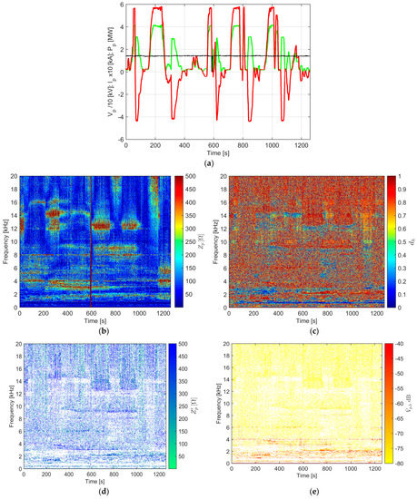
Figure 2.
Switzerland example: (a) voltage (black), current (green), and active power (red) profiles; (b) harmonic impedance Zp; (c) harmonic displacement factor dh; (d) filtered impedance Z′p; (e) normalized harmonic voltage .
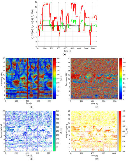
Figure 3.
France example: (a) voltage (black), current (green), and active power (red) profiles; (b) harmonic impedance Zp; (c) harmonic displacement factor dh; (d) filtered impedance Z′p; (e) normalized harmonic voltage .
- a diagram with voltage (black), current (green), and active power (red) profiles, scaled to accommodate them compactly in the same graph,
- two 2-D plots versus time and frequency of the harmonic impedance Zp and harmonic displacement factor dh using color-coded intensity,
- two post-processed 2-D plots, where the filtered impedance Z′p and normalized harmonic voltage are shown, using two different color maps for a matter of easy discernibility with the NaN arrangement mentioned.
In Figure 2a, a neutral section is clearly visible just before 600 s with Vp falling rapidly to 0, with zero current and power absorption as well. There are frequent phases of traction and braking that alternate during the trip, as this train was in normal passenger service.
It is possible to recognize some red areas for Zp (Figure 2b) corresponding to large values of impedance and, in principle, to line resonance situations, if confirmed by the Ph map (Figure 2c) with application of Rule 4. These areas are located, for example, at about 9 and 12 kHz and extend intermittently before and after the neutral section; the resonance at about 14.5 kHz, instead, disappears after the neutral section.
The persistent horizontal line at 4 kHz is well evident as a voltage harmonic in Figure 2e, but is not backed up by a corresponding large impedance value Z′p in Figure 2d, as this is, as known, an emission of another type of train running on the same line.
In Figure 3a two neutral sections are visible, at about 400 s and 600 s, again with a drop of pantograph current and absorbed power to zero. The phases of traction and braking appear to be milder (especially braking) than in the previous case of Figure 2a. Looking more closely, the absorbed power is almost double, as the train is a high-speed TGV train without intermediate train stops.
There are several red areas of Zp (Figure 3b), which however do satisfy Rule 4 (dh ≥ 0.9), as shown by comparing with Figure 3c. The persistent horizontal lines at about 2, 4, and 6 kHz in Figure 3e are not backed up by corresponding large impedance values of Z′p in Figure 3d, and they are in fact the harmonic emissions of a 4QC converter working at 2 kHz switching frequency.
It is interesting to observe two red areas of Zp with a shape that is typical of a line resonance at about 8–9 kHz and 10–11 kHz, at time 200 s and 300 s, respectively, but they do not pass the Rule 4 verification.
At some locations, this network shows a slight deviation from the theoretically grounded assumption that resonances do not depend on train position; this occurs between the two phase-separation sections, between 500 s and 650 s. Around 11–12 kHz an approximate U shape is barely visible in the Zp graph, and it is better highlighted when combined with Ph as per Rule 4, as shown in Figure 3d,e. A slight dependency on train position is in reality possible when the line is not straight, but rather a joint with a third line segment at a junction.
Anti-resonances are also clearly visible as between 10 and 12 kHz, ascending first and then descending, centered on 200 s.
Observing Figure 4b, there is a triangularly shaped set of low values (from 12 kHz to about 18 kHz and then back to 14 kHz) indicating an anti-resonance, as the harmonic power Ph is also maximum (Figure 4c), and the values of Z′p and are at their minimum (greenish and yellowish, respectively). The triangular anti-resonance begins and ends with slightly larger values of Z′p and , and at the vertex shows its minima. Correspondingly, there is a moderately large value of Z′p at about 12 kHz, making the base of this triangular area and showing distortion values that are moderately large (around –60 dB, that is 0.1%). In the original Zp map (Figure 4b), there is a larger red area of high impedance values that do not pass the confirmation dh test of Rule 4 and disappear when considering Z′p in Figure 4d.
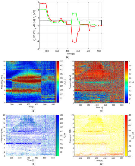
Figure 4.
Switzerland example with zoom of time-varying anti-resonance: (a) voltage (black), current (green), and active power (red) profiles; (b) harmonic impedance Zp; (c) harmonic active power Ph; (d) filtered impedance Z′p; (e) normalized harmonic voltage .
Starting from the previous tests’ cases, the behavior of the band limited THD was evaluated, as shown in Figure 5 for Switzerland and Figure 6 for France. Bands for calculation of THDi were selected depending on the characteristics of the spectrum, starting from a frequency of 500 Hz and separating the low-frequency interval from the successive bands Hi = 1 kHz located above it. THDi curves were smoothed before plotting using a moving average filter of order 11.
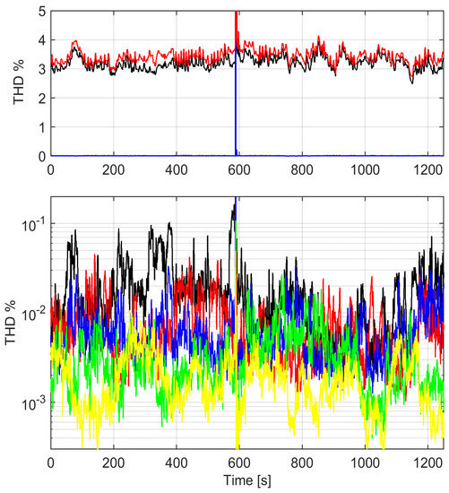
Figure 5.
Switzerland case of Figure 2 (16.7 Hz): harmonic distortion profiles THDi calculated at some frequency bands Hi = 1 kHz together with an indication of low-frequency distortion THD0 calculated over the first 500 Hz (H0 = 500 Hz). THD, THD0, THD1 (above); THD4, THD5, THD6, THD9, THD14 (below).
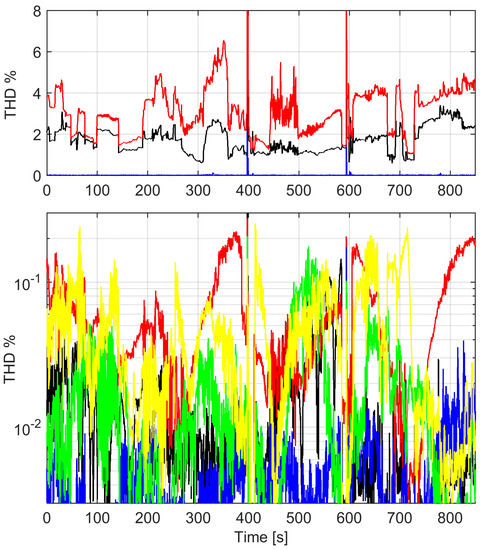
Figure 6.
France case of Figure 3 (50 Hz): harmonic distortion profiles THDi calculated at some frequency bands Hi = 1 kHz together with an indication of low-frequency distortion THD0 calculated over the first 500 Hz (H0 = 500 Hz). THD, THD0, THD1 (above); THD5, THD6, THD7, THD11, THD12 (below).
The two systems confirm their major differences, with the France AC network featuring higher distortion, and not only in the first low-frequency interval.
Resonance occurrence corresponds to time intervals with large THDi, although situations of increased rolling stock emissions also fall into this category and a clear distinction without Zp information is not possible. In addition, the prevalence of active harmonic power is an indicator that the distortion corresponds to a resonance situation, whereas without it intervals of current pulling might also be included.
The THD for Switzerland is all caused by network components in THD0, so below 500 Hz. Considering the high-frequency THD, it is evident that the THD channels of 1 kHz are not very selective in tracking resonances, as even THD14 can follow the two resonances at 13–14.5 kHz occurring in the intervals 650–800 s and 850–1000 s. The THD14 profile loses its dynamic due to other voltage components for which there is no prevalence of harmonic active power and where would have discarded. Similarly, THD9 misses the resonance at 9.5 kHz before 600 s and tracks it only between 600 and 950 s.
Observing France in Figure 6, THD7 captures two resonances at about 200 and 350 s, also visible in Figure 3e. At higher frequency, THD11 and THD12 track the two resonances at about 10.5 kHz, occurring in particular at 500 and 650 s. THD5 and THD6 should have tracked the discontinuous resonances occurring between 4.5 and 6.5 kHz, and they are partially successful, at the beginning and around 500–550 s.
5. Outline of Real-Time Implementation
The discussed method is based on electrical quantities available onboard (Vp and Ip) and processed by means of STFT, on which the ratio and the product are calculated to derive Zp and Ph, that, once normalized, gives dh. The involved operations are thus basic operations available in a wide range of microcontrollers and microprocessors. The processing to produce the figures in Section 4 was purposely performed using a large number of bins on the frequency axis with a 8 Hz frequency resolution for graphical reasons; what is discussed in the following is the optimization of time and frequency resolution, as well as the size of matrices to fit available memory and process data in real time. Real time is defined as a time frame suitable to feedback on the monitored system following the detection of events that trigger a control action. In the present case, the identification of an incipient major resonance condition with increasing overvoltage caused by distortion should trigger a change of the rolling stock operating conditions, besides tagging the chainage position for later inspection. An estimate of the real-time requirement can be based on experience and confirmed by plots of resonance conditions vs. time that are available in the literature; Figure 3 in [9] shows an almost linear increase in line voltage between 28 kV at 9:35 am and more than 30 kV at 9:36 am. A detection and action time of some seconds is thus suitable for real-time reaction to these types of phenomena.
The discussion begins with a flowchart and description of data structures (Figure 7).
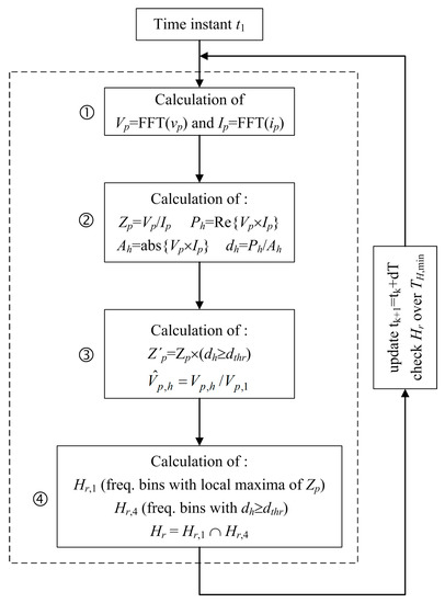
Figure 7.
Flowchart of the harmonic resonance detection method and data structures used to support estimate of computational and storage complexity.
The number of points N is determined by the sampling frequency fs and the frequency resolution df: N = fs/df (of course, N is an integer and should be rounded if needed). Then, the sampling frequency must be set to a minimum of twice the maximum frequency that is to be evaluated. In our case, we also reasoned on components that are slightly above 10 kHz, which implies fs ≥ 25 kSa/s (in Section 4 the value of fs was 50 kSa/s).
Keeping df = 16.7 Hz (T = 60 ms), the resulting N ranges between 1500 and 3000 for fs ranging between 25 and 50 kSa/s. Let’s assume the same fs of Section 4 and N = 3000.
Such calculation can be accommodated in any DSP or microcontroller with a math core. For the ongoing discussion, a basic 10 MFlops floating-point calculation speed may be considered, as reserved for running the algorithm (“Flops” stands for floating point operations per second); it is a small fraction of the whole DSP calculation performance in excess of several hundred MFlops (exemplified by [48,49] covering almost 20 years of DSP production). For complex operations, a factor of four should be considered for multiplication or division, and a factor of two for summation. A reserved 10 MWords memory area may be also assumed, having for simplicity indicated with “words” a unit suitable for a single-precision floating point number; although, in case of 32-bit words a double-precision floating point number requires two words. Similarly, this reference memory budget is a small fraction of the total system memory, that can range up to several hundred MB.
At every time instant tk the vectors Vp and Ip are calculated with a fast Fourier transform (FFT) of N points and the complexity, as known, is in the order of 1.5Nlog2N. This amounts to 52k Flops for the two N values, to be multiplied by four assuming all operations are complex multiplications, resulting in 2.1% of the 10 MFlops basic calculation speed. The occupied memory is 2N words for each complex vector, so 12 kWords, or 0.12%.
Calculation of Zp, then, requires (2 + 2 + 1)N for the absolute value of the numerator and denominator, separately, with two square roots (single CPU instruction with a math coprocessor) and a ratio of real vectors, so another 3N, which is in total 8N Flops (24 kFlops, or 0.24%). The necessary memory is 2N words as a complex vector.
Calculation of Ph requires the calculation of apparent power An (with the same complexity of Zp) and the extraction of the real part that has no complexity. The, for dh, reusing the pre-calculated An (that must be stored somewhere in memory, requiring 2N words, or 6 kWords), there is only the ratio of the absolute values of Pn and An, so N Flops.
Calculation of data structures Z′p and is accomplished by a comparison and flagging for the former (2N operations) and by a scalar division for the latter, in total 3N Flops, and the storage of two real vectors (2N words).
The check of Zp local peaks and large positive values of dh, with creation of sets Hr,1 and Hr,4, needs some amount of code, possibly implementing a local peak search with comparison with neighbors, so some number of operations that may be collectively estimated to about 10N. The storage is that of the new sets Hr,1 and Hr,4, and then the resulting Hr as intersection, in total up to 3N Words.
Calculations of the frequency vectors are repeated every dT seconds and the resulting vectors may be stored in adjacent memory areas to ease the comparison over the time axis. Time resolution is not demanding and dT may be chosen as a minimum equal to 300 ms for uniformity, between 16.7, 50 and 60 Hz systems, corresponding to 25 m of train movement at 300 km/h (equal to the length of one coach). Longer time intervals may be selected as well, easing computational and storage necessities and providing an adequate space resolution. Confirmation of persistence of a resonance, as commented in Section 4, is achieved if the conditions shown in Rules 1 to 4 persist, e.g., for tens of seconds, corresponding to about 1 km of traveled line at 300 km/h. Such an interval of observation Ttot represents the number of vectors stored in memory in a circular fashion, beyond which the oldest ones are replaced by the newest ones. The depth of the circular buffer will thus be B = Ttot/dT, corresponding to about 33 for the exemplified choices of dT and Ttot. Correspondingly, the number of repeated calculations over 1 s, M, is given by M = 1/dT, equal to three in the present case.
The check of persistency of membership of indexes to the set Hr (to last longer than TH,min) can be achieved with some logic operations, that collectively will not take more than N Flops at each time instant (in fact, Hr,1, Hr,4 and Hr are always quite sparse, possibly filled up to some % maximum).
By showing figures below 100% in the last row of Table 2, it is demonstrated that the allocated 10 MFlops and 10 MWords are sufficient for the implementation of the proposed method in real time. In case of increased requirements, e.g., a more complete representation or additional verifications, the computational and storage requirements should be scaled correspondingly.
Table 2.
Summary of estimated computational and memory budget (fs = 50 kSa/s, N = 3000). Algorithm steps are numbered as in the flowchart of Figure 7.
6. Conclusions
This work has discussed the problem of detection of resonances in AC railways in a rolling stock perspective, starting from the measured pantograph quantities (voltage and current) and using the derived quantities of pantograph impedance and harmonic active power. Suitable conditions are identified for the detection of resonance, focusing on parallel resonances, and a set of rules has been formulated. Local maxima of the pantograph impedance are detected and confirmed by a prevalent flow of harmonic active power, indicating the mutual cancellation of the harmonic reactive power terms. Such a condition for the harmonic active power also persists in the case of series resonance, for which minima of the pantograph impedance should be considered (an example is given in Figure 4). In both cases, further confirmation is obtained by the amplification of the harmonic components of voltage and current, respectively.
Rules are synthesized for the maxima of pantograph impedance Zp and for the normalized harmonic active power (called harmonic displacement factor dh) to be larger than a convenient threshold (which for the demonstration was set to 0.9). These criteria have then been validated by means of extensive experimental data measured in two different AC railway networks, one operated at 16.7 Hz (Switzerland) and one at 50 Hz (France).
The straightforward monitoring of voltage harmonic distortion was also included and compared to results in [18]. Although it is a useful indicator in general, it has issues of selectivity, due to the mix of voltage harmonic components with opposite or incoherent behavior not being able to reject those without a large active power fraction. It also always necessitates some degree of smoothing during post-processing to improve readability of obtained distortion profiles versus time. It has, however, a simple implementation, especially if implemented with a filter bank.
The comparison of voltage harmonic distortion over selected frequency bands with the results previously obtained with the pantograph impedance, combined with the harmonic displacement factor, has shown the superiority of the latter in terms of ability to locate and track resonance phenomena, avoiding the interference of spectral components of a reactive nature.
Author Contributions
Investigation, A.M. and L.S.; Methodology, A.M. and L.S.; Software, A.M. and L.S.; Writing—original draft, A.M.; Writing—review & editing, A.M. and L.S. All authors have read and agreed to the published version of the manuscript.
Funding
This research received no external funding.
Institutional Review Board Statement
Not applicable.
Conflicts of Interest
The authors declare no conflict of interest.
References
- Kaleybar, H.J.; Brenna, M.; Foiadelli, F.; Fazel, S.S.; Zaninelli, D. Power Quality Phenomena in Electric Railway Power Supply Systems: An Exhaustive Framework and Classification. Energies 2020, 13, 6662. [Google Scholar] [CrossRef]
- EN. Railway Applications—Power Supply and Rolling Stock—Technical Criteria for the Coordination between Power Supply (Substation) and Rolling Stock to Achieve Interoperability; EN 50388; CENELEC: Brussels, Belgium, 2013. [Google Scholar]
- EN. Railway Applications—Fixed Installations and Rolling Stock—Technical Criteria for the Coordination between Traction Power Supply and Rolling Stock to Achieve Interoperability—Part 1: General; EN 50388-1; CENELEC: Brussels, Belgium, 2017. [Google Scholar]
- Gazafrudi, S.M.M.; Tabakhpour, L.A.; Fuchs, E.F.; Al-Haddad, K. Power quality issues in railway electrification: A comprehensive perspective. IEEE Trans. Ind. Electron. 2015, 62, 3081–3090. [Google Scholar] [CrossRef]
- Roudsari, H.M.; Jamali, S.; Jalilian, A. Dynamic modeling, control design and stability analysis of railway active power quality conditioner. Electr. Power Syst. Res. 2018, 160, 71–88. [Google Scholar] [CrossRef]
- Panpean, C.; Areerak, K.; Santiprapan, P.; Areerak, K.; Shen Yeoh, S. Harmonic Mitigation in Electric Railway Systems Using Improved Model Predictive Control. Energies 2021, 14, 2012. [Google Scholar] [CrossRef]
- Morais, V.A.; Afonso, J.L.; Carvalho, A.S.; Martins, A.P. New Reactive Power Compensation Strategies for Railway Infrastructure Capacity Increasing. Energies 2020, 13, 4379. [Google Scholar] [CrossRef]
- Tanta, M.; Cunha, J.; Barros, L.A.M.; Monteiro, V.; Pinto, J.G.O.; Martins, A.P.; Afonso, J.L. Experimental Validation of a Reduced-Scale Rail Power Conditioner Based on Modular Multilevel Converter for AC Railway Power Grids. Energies 2021, 14, 484. [Google Scholar] [CrossRef]
- Song, K.; Wu, M.; Yang, S.; Liu, Q.; Agelidis, V.G.; Konstantinou, G. High-Order Harmonic Resonances in Traction Power Supplies: A Review Based on Railway Operational Data, Measurements, and Experience. IEEE Trans. Power Electron. 2020, 35, 2501–2518. [Google Scholar] [CrossRef]
- Jiang, X.; He, Z.; Hu, H.; Zhang, Y. Analysis of the Electric Locomotives Neutral-section Passing Harmonic Resonance. Energy Power Eng. 2013, 5, 546–551. [Google Scholar] [CrossRef]
- Liu, Q.; Sun, B.; Yang, Q.; Wu, M.; He, T. Harmonic Overvoltage Analysis of Electric Railways in a Wide Frequency Range Based on Relative Frequency Relationships of the Vehicle–Grid Coupling System. Energies 2020, 13, 6672. [Google Scholar] [CrossRef]
- Chu, X.; Lin, F.; Yang, Z. The Analysis of Time-Varying Resonances in the Power Supply Line of High Speed Trains. In Proceedings of the Internet Power Electronics Conference, Hiroshima, Japan, 18–21 May 2014. [Google Scholar] [CrossRef]
- Lutrakulwattana, B.; Konghirun, M.; Sangswang, A. Harmonic resonance assessment of 1 × 25kV, 50Hz traction power supply system for Suvarnabhumi airport rail link. In Proceedings of the 18th International Conference on Electrical Machines and Systems (ICEMS), Pattaya, Thailand, 25–28 October 2015. [Google Scholar]
- Holtz, J.; Kelin, H.J. The propagation of harmonic currents generated by inverter-fed locomotives in the distributed overhead supply system. IEEE Trans. Power Electron. 1989, 4, 168–174. [Google Scholar] [CrossRef]
- Sainz, L.; Monjo, L.; Riera, S.; Pedra, J. Study of the Steinmetz Circuit Influence on AC Traction System Resonance. IEEE Trans. Power Deliv. 2012, 27, 2295–2303. [Google Scholar] [CrossRef]
- Brenna, M.; Capasso, A.; Falvo, M.C.; Foiadelli, F.; Lamedica, R.; Zaninelli, D. Investigation of resonance phenomena in high speed railway supply systems: Theoretical and experimental analysis. Electr. Power Syst. Res. 2011, 81, 1915–1923. [Google Scholar] [CrossRef]
- Kolar, V.; Palecek, J.; Kocman, S.; Trung, T.Y.; Orsag, P.; Styskala, V.; Hrbac, R. Interference between Electric Traction Supply Network and Distribution Power Network Resonance Phenomenon. In Proceedings of the 14th International Conference on Harmonics and Quality of Power (ICHQP), Bergamo, Italy, 26–29 September 2010. [Google Scholar] [CrossRef]
- Lee, H.; Lee, C.; Jang, G.; Kwon, S. Harmonic analysis of the Korean high-speed railway using the eight-port representation model. IEEE Trans. Power Deliv. 2006, 21, 979–986. [Google Scholar] [CrossRef]
- Li, J.; Wu, M.; Molinas, M.; Song, K.; Liu, Q. Assessing High-Order Harmonic Resonance in Locomotive-Network Based on the Impedance Method. IEEE Access 2019, 7, 68119–68131. [Google Scholar] [CrossRef]
- Hu, H.; Shao, Y.; Tang, L.; Ma, J.; He, Z.; Gao, S. Overview of Harmonic and Resonance in Railway Electrification Systems. IEEE Trans. Ind. Appl. 2018, 54, 5227–5245. [Google Scholar] [CrossRef]
- Gao, S.; Li, X.; Ma, X.; Hu, H.; He, Z.; Yang, J. Measurement-Based Compartmental Modeling of Harmonic Sources in Traction Power-Supply System. IEEE Trans. Power Deliv. 2017, 32, 900–909. [Google Scholar] [CrossRef]
- Hu, H.; Tao, H.; Blaabjerg, F.; Wang, X.; He, Z.; Gao, S. Train–Network Interactions and Stability Evaluation in High-Speed Railways–Part I: Phenomena and Modeling. IEEE Trans. Power Electron. 2018, 33, 4627–4642. [Google Scholar] [CrossRef]
- Zhang, G.; Liu, Z.; Yao, S.; Liao, Y.; Xiang, C. Suppression of Low-Frequency Oscillation in Traction Network of High-Speed Railway Based on Auto-Disturbance Rejection Control. IEEE Trans. Transp. Electrif. 2016, 2, 244–255. [Google Scholar] [CrossRef]
- Hemmer, B.; Mariscotti, A.; Wuergler, D. Recommendations for the calculation of the total disturbing return current from electric traction vehicles. IEEE Trans. Power Deliv. 2004, 19, 1190–1197. [Google Scholar] [CrossRef]
- Meyer, M.; Schöning, J. Netzstabilität in grossen Bahnnetzen. Schweiz. Eisenb.-Rev. Eisenb.-Rev. Int. 1999, 7, 312–317. [Google Scholar]
- Pröls, M.; Strobl, B. Stabiltätskriterien für Wechselwirkungen mit Umrichteranlagen in Bahnsystemen. Elektr. Bahnen 2006, 104, 542–552. [Google Scholar]
- Mollerstedt, E.; Bernhardsson, B. Out of control because of harmonics an analysis of the harmonic response of an inverter locomotive. IEEE Control Syst. Mag. 2000, 20, 70–81. [Google Scholar] [CrossRef]
- Li, T.; Wu, G.; Zhou, L.; Gao, G.; Wang, W.; Wang, B.; Liu, D.; Li, D. Pantograph Arcing’s Impact on Locomotive Equipments. In Proceedings of the IEEE 57th Holm Conference on Electrical Contacts (Holm), Minneapolis, MN, USA, 11–14 September 2011. [Google Scholar] [CrossRef]
- Bongiorno, J.; Mariscotti, A. Experimental validation of the electric network model of the Italian 2 × 25 kV 50 Hz railway. In Proceedings of the 20th IMEKO TC4 Symposium on Measurements of Electrical Quantities, Benevento, Italy, 15–17 September 2014. [Google Scholar]
- Liu, Y.; Xu, J.; Shuai, Z.; Li, Y.; Peng, Y.; Liang, C.; Cui, G.; Hu, S.; Zhang, M.; Xie, B. A Novel Harmonic Suppression Traction Transformer with Integrated Filtering Inductors for Railway Systems. Energies 2020, 13, 473. [Google Scholar] [CrossRef] [Green Version]
- Zhang, R.; Lin, F.; Yang, Z.; Cao, H.; Liu, Y. A Harmonic Resonance Suppression Strategy for a High-Speed Railway Traction Power Supply System with a SHE-PWM Four-Quadrant Converter Based on Active-Set Secondary Optimization. Energies 2017, 10, 1567. [Google Scholar] [CrossRef]
- Liu, Q.; Li, J.; Wu, M. Field Tests for Evaluating the Inherent High-Order Harmonic Resonance of Traction Power Supply Systems up to 5000 Hz. IEEE Access 2020, 8, 52395–52403. [Google Scholar] [CrossRef]
- Mariscotti, A.; Pozzobon, P.; Vanti, M. Simplified modelling of 2 × 25 kV AT Railway System for the solution of low frequency and large scale problems. IEEE Trans. Power Deliv. 2007, 22, 296–301. [Google Scholar] [CrossRef]
- Pilo, E.; Rouco, L.; Fernández, A.; Abrahamsson, L. A Monovoltage Equivalent Model of Bi-Voltage Autotransformer-Based Electrical Systems in Railways. IEEE Trans. Power Deliv. 2012, 27, 699–708. [Google Scholar] [CrossRef]
- Bottenberg, A.; Debruyne, C.; Peterson, B.; Rens, J.; Knockaert, J.; Desmet, J. Network resonance detection using harmonic active power. In Proceedings of the 18th International Conference on Harmonics and Quality of Power (ICHQP), Ljubljana, Slovenia, 13–16 May 2018. [Google Scholar] [CrossRef]
- Mariscotti, A. Impact of Harmonic Power Terms on the Energy Measurement in AC Railways. IEEE Trans. Instrum. Meas. 2020, 69, 6731–6738. [Google Scholar] [CrossRef]
- Filippone, F.; Mariscotti, A.; Pozzobon, P. The Internal Impedance of Traction Rails for DC Railways in the 1-100 kHz Frequency Range. IEEE Trans. Instrum. Meas. 2006, 55, 1616–1619. [Google Scholar] [CrossRef]
- Mariscotti, A.; Pozzobon, P. Measurement of the Internal Impedance of Traction Rails at Audiofrequency. IEEE Trans. Instrum. Meas. 2004, 53, 792–797. [Google Scholar] [CrossRef]
- Robert, A.; Deflandre, T.; Gunther, E.; Bergeron, R.; Emanuel, A.; Ferrante, A.; Finlay, G.S.; Gretsch, R.; Guarini, A.; Iglesias, J.G.; et al. Guide for assessing the network harmonic impedance. In Proceedings of the 14th International Conference and Exhibition on Electricity Distribution (Part 1), Birmingham, UK, 2–5 June 1997. [Google Scholar] [CrossRef]
- Kannan, S.; Meyer, J. Recent Developments in Harmonic Resonance Detection in Low Voltage Networks using Impedance Measurement Techniques. In Proceedings of the 8th International Conference on Power Systems (ICPS), Jaipur, India, 20–22 December 2019. [Google Scholar] [CrossRef]
- Ritzmann, D.; Wright, P.S.; Holderbaum, W.; Potter, B. A method for accurate transmission line impedance parameter estimation. IEEE Trans. Instrum. Meas. 2016, 65, 2204–2213. [Google Scholar] [CrossRef]
- Mariscotti, A. Experimental characterization of active and nonactive harmonic power flow of AC rolling stock and interaction with the supply network. IET Electr. Syst. Transp. 2021, 11, 109–120. [Google Scholar] [CrossRef]
- Mariscotti, A. Behavior of Single-Point Harmonic Producer Indicators in Electrified AC Railways. Metrol. Meas. Syst. 2020, 27, 641–657. [Google Scholar] [CrossRef]
- Lodetti, S.; Bruna, J.; Melero, J.J.; Khokhlov, V.; Meyer, J. A Robust Wavelet-Based Hybrid Method for the Simultaneous Measurement of Harmonic and Supraharmonic Distortion. IEEE Trans. Instrum. Meas. 2020, 69, 6704–6712. [Google Scholar] [CrossRef]
- Mariscotti, A. Methods for Ripple Index evaluation in DC Low Voltage Distribution Networks. In Proceedings of the IEEE International Measurement Technology Conference IMTC, Warsaw, Poland, 1–3 May 2007. [Google Scholar] [CrossRef]
- Mariscotti, A. Data sets of measured pantograph voltage and current of European AC railways. Data Brief 2020, 30, 105477. [Google Scholar] [CrossRef] [PubMed]
- Mariscotti, A. Direct Measurement of Power Quality over Railway Networks with Results of a 16.7 Hz Network. IEEE Trans. Instrum. Meas. 2011, 60, 1604–1612. [Google Scholar] [CrossRef]
- Texas Instruments, SM320C6712 Floating Point Digital Signal Processors. September 2004. Available online: https://www.ti.com/lit/gpn/SM320C6712D-EP (accessed on 19 August 2021).
- Texas Instruments, TMS320C6652 and TMS320C6654 Fixed and Floating-Point Digital Signal Processor. October 2019. Available online: https://www.ti.com/lit/gpn/tms320c6652 (accessed on 19 August 2021).
Publisher’s Note: MDPI stays neutral with regard to jurisdictional claims in published maps and institutional affiliations. |
© 2021 by the authors. Licensee MDPI, Basel, Switzerland. This article is an open access article distributed under the terms and conditions of the Creative Commons Attribution (CC BY) license (https://creativecommons.org/licenses/by/4.0/).