Abstract
The solution of multiphysical problems in the field of electrical machines is a complex task that involves the modeling of a wide variety of coupled physical domains. Different types of models and solution methods can be used to model and solve the individual domains. In this paper a procedure for the methodical selection of the most suitable model for a given multiphysics task is presented. Furthermore, an approach for the selection of the most suitable variable machine parameters for a design optimization is presented. The model selection is presented on the basis of the electromagnetic calculation of an induction machine. For this purpose, models of different value ranges and levels of detail, such as analytical and numerical ones, are considered. The approach of the model selection is explained and applied on the basis of a coupled electromagnetic-thermal simulation of an exemplary induction machine. The results show that the model selection presented here can be used to methodically determine the most suitable model in terms of its value range, level of detail and computational effort for a given multiphysical problem.
1. Introduction
Complex tasks in the field of electrical machines usually comprise several physical domains and thus form a multiphysics problem. The aim of modeling and calculating multiphysics problems is to represent all physical effects of the individual domains that are relevant for the application. In a multiphysics problem, the individual domains can be independent or coupled. In [1], coupled problems are defined as those involving multiple domains and dependent variable sets that usually, but not necessarily, describe different physical effects, and where either no domain can be solved correctly independently of the other domains or none of the dependent variable sets can be eliminated explicitly. An example of such a coupled multiphysics problem is the thermal simulation of an operating point of an electrical machine. Here, among other things, the domains of electromagnetism and thermal are bidirectionally dependent on each other.
If electrical machines are not considered as an independent system, but as part of a system of several components from different fields of technology, the complexity of the coupled multiphysics problem increases. An example of such a system is an electric drive train. The individual components of the system, such as electric motor, gearbox or battery, can in turn be assigned to individual domains or divided into several domains.
Different models are used for modeling and calculating the individual components and their domains, depending on the required accuracy and the physical effects to be modeled. The individual models therefore differ in their value range and level of detail of the representation of the physical effects as well as in their computational or solution effort. They can be classified into the categories of empirical, analytical, lumped parameter, and numerical models. The exemplary classification in value range, level of detail and computational effort for models for the electromagnetic simulation of an Induction Machine (IM) used in this paper are shown in Figure 1. Analytical models such as the Fundamental Wave Model (FWM) or Harmonic Wave Model (HWM) have a smaller value range of modeled physical effects and a lower level of detail of individual effects than numerical models such as the Finite Element Method (FEM), but also a lower computational effort.
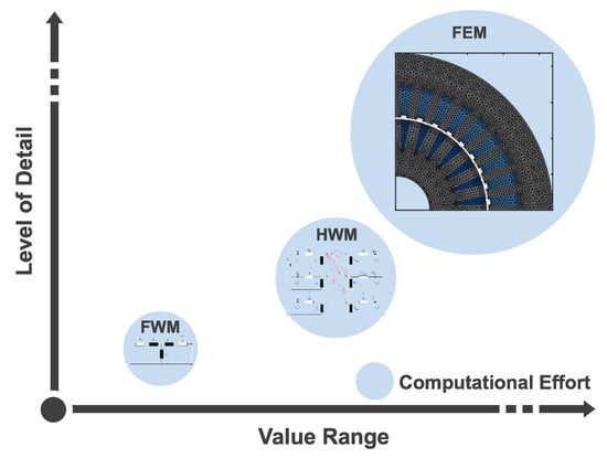
Figure 1.
Classification of IM models with respect to value range, level of detail, and computational effort.
Examples of models, methods, and physical effects considered for solving multiphysics problems in the field of electrical machines are explained in [2]. There, a modular computational approach for the calculation, simulation, and design of electrical machines is presented, which has been and is being applied in several scientific papers.
For the computation and simulation of the aforementioned multiphysics and coupled problems, the question arises as to which models are most suitable for which domains. Suitability refers to the fact that the particular model can represent the desired effects at an appropriate level of detail and is computationally efficient. The respective suitability of a model is strongly problem-dependent, since different problems require the modeling of various effects with different degrees of accuracy. Due to its high computational effort, the selection of the most complex model in the respective domain is not always the means of choice, especially in the design process of the machine or the overall system. Furthermore, the sensitivity with respect to the coupling variables is a necessary requirement of the used models.
In view of the modular computational approach mentioned above, the question of efficient model selection may arise in many of the calculation columns listed. For example, which electromagnetic and thermal models can be used for the thermal calculation of the electrical machine and which electromagnetic and structural dynamics models can be used for the Noise Vibration Harshness (NVH) analysis?
Design and redesign processes of electrical machines are also performed with the help of multilevel mathematical optimization algorithms. Here, the choice of the model in the individual optimization stages is an important factor influencing the quality of the result and the computational efficiency. These parameters also depend on the choice of optimization variables.
In the publications mentioned, models are mostly used without evaluating their suitability or advantages and disadvantages for solving the problem in comparison with other models. A methodical selection of the used model is not considered in detail. Therefore, such a methodological approach to model selection is addressed in this paper and presented using the electromagnetic simulation of IM as an example.
By specifying a few parameters, such as the desired effects to be modeled and their level of detail, the method offers the possibility to automatically select the model that meets the requirements and has the lowest computational cost. The selection method is based on the analysis of an exemplary IM for a given power, torque, and speed range in certain operating points and the derived ranges of values, levels of detail, and degrees of freedom of each machine model. The model selection can then be applied to problems requiring simulations of machines in a similar power, torque and speed range, and similar geometric dimensions. The proposed model selection approach can also be used in machine optimization problems in which machines of similar power range but different designs are simulated to determine the appropriate models in individual optimization stages. Such an example is given in [3]. In such optimization environments, the choice of optimization parameters is crucial and can also be done methodically. For this purpose, an approach for parameter selection is presented in this paper, which ensures an efficient design and redesign optimization.
The paper is organized as follows. First, the models of an IM considered in the model selection are introduced. These include the FWM, the HWM according to [4,5,6], and an Extended Harmonic Wave Model (E-HWM) developed in this work to consider saturation, three analytical models, and the Time Harmonic Finite Element Model (TH-FEM) and Transient Finite Element Model (T-FEM), two numerical models. Afterward, the approach of the model selection is presented. The input parameters of the methodology and the procedure for the analysis of the value ranges, levels of detail, and computational efforts of the models are discussed. In the following, the parameter selection, which can be applied in optimization environments, is presented. Subsequently, the approach for the model selection is applied on the basis of an exemplary problem. As an example, a weakly coupled electromagnetic-thermal simulation of an IM is used to analyze the thermal operating behavior of the machine. The parameter selection in combination with the model selection is applied in [3] in an optimization of the machine design of an IM.
2. Induction Machine Models
In order to apply the model selection approach presented later to the example of the electromagnetic simulation of an IM, different models with different ranges of values and levels of detail are necessary. In this paper, five different models of an IM are considered. These include the FWM, the HWM, and an E-HWM, three analytical machine models, and the TH-FEM and T-FEM, two numerical models. They are briefly described below. The order corresponds to an increasing value range and level of detail. At the end of this section, the iron loss model used by all models is described.
2.1. Fundamental Wave Model
Modeling of a squirrel cage IM in the FWM is performed using the single-phase Equivalent Circuit Diagram (ECD) presented in Figure 2. In this paper, the T-ECD is used, which allows the consideration of saturation in terms of a current-dependent main inductance. The use of a stator flux or rotor flux based ECD is also possible but is not applied here. The ECD is composed of the stator resistance , the rotor resistance divided by the slip s, the leakage reactances and , and the main reactance . The rotor-side quantities related to the stator by the transmission factor are thereby characterized by a. For the calculation of these elements of the ECD, which can be derived exclusively from the machine geometry and constant parameters, reference is made to the literature [7]. Important physical quantities and effects which affect the range of values or the level of detail of the machine modeling are briefly explained.
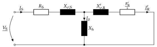
Figure 2.
Representation of the single-phase ECD of the IM with a squirrel cage rotor.
2.1.1. Rotor Resistance
To consider the short circuit ring of the squirrel cage, the bar resistance and the ring resistance component are used to calculate the two dimensional rotor resistance . The latter results from the transformation of the resistance of a ring section into a series equivalent resistance. The rotor resistance is thus given by:
This procedure is also used for the calculation of the rotor resistance in the other machine models. A more detailed derivation of the rotor resistance for 2D modeling is given in [8].
2.1.2. Leakage Inductances
The magnetic coupling of a winding with itself is described by the leakage inductance . This coupling manifests itself in a reduction of the main flux. The essential parts of the leakage flux are the harmonic, the slot and end-face leakage flux, and the leakage flux in the tooth tip space. These effects are considered in an analytically calculated leakage flux factor when calculating the stator and rotor inductances.
2.1.3. Main Inductance and Saturation
By calculating the main inductance via the flux linkage, it is possible to consider the material saturation of the stator and rotor laminations of the IM. With a magnetic ECD of the machine geometry, the magnetic flux densities B and magnetic voltages V in the teeth () and yokes () of the stator () and rotor () and in the air gap () are calculated. The saturated main inductance is obtained by dividing the operating point specific main flux linkage by the magnetizing current :
The factor describes the total winding factor including the distribution and pitch factors, the number of windings per phase, and p the number of pole pairs.
2.1.4. Iron Losses
The iron losses for all models in this paper are calculated using the IEM-Formula, which will be presented later in the paper. For the calculation of the iron losses, the magnetic flux density in the stator and rotor lamination is of interest. The calculation of tooth and yoke flux densities in the FWM is done by the magnetic ECD. Since a local resolution of the iron losses in the stator and rotor laminations is not possible in the FWM, the flux density in tooth and yoke is assumed to be constant and its local mean value is determined accordingly. In this model, only the fundamental component of the magnetic flux density can be calculated, which results in the neglect of the iron losses due to higher flux density harmonics.
2.2. Harmonic Wave Model
The operating behavior, in particular the electromagnetic torque, the electromagnetic forces, and the ohmic and iron losses of an IM is significantly influenced by the orders and amplitudes of the harmonics that occur. These harmonics cannot be modeled in the FWM. Therefore, the HWM considering the multiple armature reaction provides a possibility for the analytical description of these effects [4,5,6]. Assuming a sinusoidal stator current, the discrete distribution of the stator windings, neglecting the slot openings, results in non-sinusoidal stator Magnetomotive Force (MMF) in the form of a staircase function. The currents of different order and amplitude induced in the rotor by this stator field, in turn, each generate staircase-shaped rotor MMF, which in turn induces new voltages in the stator (primary armature reaction). The harmonic model according to [4,5,6] additionally considers the secondary, tertiary, and quaternary armature reaction [9]. In addition to the multiple armature reaction, further effects causing harmonics, such as stator and rotor slotting or rotor eccentricity, can be considered. Due to the assumption of an infinitely high iron permeability saturation harmonics cannot be represented in this HWM. Further important physical quantities and effects affecting the value range or the level of detail of the machine modeled with the HWM are briefly explained.
2.2.1. Current Displacement
Due to the consideration of higher-order harmonics and the resulting high frequencies, current displacement must also be considered. While this effect is negligible in the stator with round wire windings due to the relatively high penetration depths at the frequencies considered [10], the influence in the rotor must be considered by a frequency-dependent reduction factor, since the bars represent solid conductors in the iron packet [11].
2.2.2. Slot Openings in the Stator and Rotor
The slot openings in the stator and rotor can be considered in the form of a permeance function for a better description of the field characteristics [11,12]. Among other things, this increases the accuracy of the calculation of the iron losses and the distribution of forces in the machine. The permeance function is described as the product of the permeance functions of stator and rotor, which can be represented as infinite complex Fourier series due to the periodicity [4,11,12].
Accounting for these effects in combination with multiple armature reaction leads to a good approximation of the field behavior, which is illustrated in Figure 3 for the local variation of the air gap flux density compared to a linear T-FEM simulation.
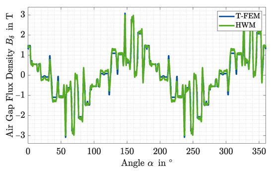
Figure 3.
Simulated air gap flux density of an IM with linear stator and rotor magnetic material properties using the T-FEM and HWM.
2.2.3. Iron Losses
For the calculation of the iron losses in the HWM, which includes losses due to higher harmonics, the time-dependent magnetic flux density in the stator and rotor lamination is of interest. The calculation of tooth and yoke flux densities in the HWM is done by an integral approach. Since a local resolution of the iron losses in the stator and rotor laminations is also not possible in the HWM, the flux density in tooth and yoke is assumed to be constant, as in the magnetic ECD used in the FWM, and its local mean value is determined accordingly. For this purpose, it is assumed for the determination of the tooth flux density , that the entire magnetic flux in the area of a slot pitch flows through the corresponding tooth.
By integrating the air gap flux density over a stator or rotor slot pitch, the magnetic flux in the respective tooth can be determined. Since no location dependence in the tooth is considered, the area integral for calculating the tooth flux from the tooth flux density can be replaced by a multiplication with the toot width and active axial length so that the tooth flux density follows from
with N being the number of slots and r being the middle radius of the air gap.
The assumption underlying the calculation of the yoke flux densities describes that the magnetic flux is equally distributed over both paths in the yoke via a pole pitch, which is why half the air gap flux is present in each case. By converting the area integral for the determination of the yoke flux from the yoke flux density into a multiplication with the yoke height and the yoke flux density results in
2.3. Extended Harmonic Wave Model
The neglect of the iron saturation in the HWM according to [4,5,6] represents an essential limitation in the operating point calculation of the IM. Therefore, an E-HWM is introduced in this paper, which provides an approach to account for the iron saturation.
2.3.1. Approach
If the influence of the iron saturation on the harmonics is to be considered, the flattening of the hysteresis curve in the nonlinear region and the resulting flattening of the air gap flux density must be modeled, which is shown for the idealized case of a sinusoidal air gap flux density in the middle plot of Figure 4. This can be realized mathematically by a circumferential location dependent description of an effective air gap. Here, as a consequence of the main field saturation, the air gap is increased on average by a saturation factor . In the region of large iron saturation, i.e., at the maximum of the air gap flux density , the air gap is increased by another saturation factor and decreased at zero crossings. Thus, the time- and location-dependent air gap conductance function shown in the left plot of Figure 4 can be defined. This moves synchronously with the fundamental wave field and therefore results in
where the factor of two in the cosine argument is a consequence of the simultaneous iron saturation by the north and south poles of the air gap field. The flattened airgap flux density follows from multiplying the original airgap flux density by the airgap conductance function given by
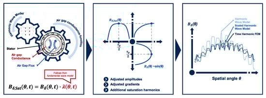
Figure 4.
Approach of the consideration of saturation in the E-HWM.
In the right plot of the Figure 4 exemplary flux density curves simulated by a TH-FEM, a HWM, and an E-HWM are shown. Here the effect of the flattening of the flux density by the application of the air gap conductance function can be seen.
2.3.2. Calculation of the Air Gap Conductance Function
The derivation of the saturation factors and is done using the FWM. By dividing the amplitude of the air gap flux density of the FWM by the fundamental wave of the HWM the scaling factor
at maximum saturation can be calculated. This factor thus represents the minimum of the air gap conductance function. Assuming a cosine fundamental wave, the amplitude can be expressed as
and thus describes the part of a period that the magnitude of the fundamental wave of the HWM is above the amplitude of the air gap flux density of the FWM, related to the scaling factor at maximum saturation. The larger this part, the greater the difference between the saturated and unsaturated regions, and thus the amplitude of the air gap conductance function. The mean value follows from the addition of the minimum and amplitude. Therefore can be expressed as
To consider the saturation effects on the curves of the flux densities in the HWM, the calculated time and local curves of the air gap flux density, as well as the time curves of the tooth and yoke flux densities, can be multiplied by the function resulting from (7). For the latter progressions, the scaling factors at maximum saturation must thereby be calculated with the amplitudes of the tooth and yoke flux densities of the FWM and HWM, respectively, resulting in different scaling functions than in the air gap.
The introduction of saturation phenomena in the iron loss calculation in the E-HWM is based on the scaling of existing harmonics as well as the consideration of additional saturation harmonics [7]. From (8), with the help of trigonometric relations, the scaling of existing harmonics can be converted to
where the fundamental is scaled differently from the other harmonics. The derivation of the additional saturation harmonics is done analogously. The flattening of the air gap flux density results in particular in a dominant third harmonic, which is calculated differently from the other saturation harmonics. In general, the n-th harmonic results in two additional saturation harmonics with the order . Their amplitudes result in
Since a change in the flux densities also results in new induced currents in the rotor, an iterative adaptation in the E-HWM is required. For this purpose, starting from the scaled flux densities, the rotor current is updated, which in turn changes the flux densities. The updated flux densities are scaled again, and so on. To adjust the induced rotor current, a constant scaling factor is applied according to
by which the inductances are multiplied. Based on the scaled inductances, the rotor current can be updated. By integrating a relaxation factor, the convergence behavior of the successive substitution can also be improved. In Figure 5 the same operating point of an exemplary IM as in Figure 3 is simulated using non linear magnetic material properties. The air gap flux density compared to the linear material in Figure 3 differs strongly. Nevertheless, the use of the E-HWM makes it possible to simulate the saturation-dependent flux density approximately well.
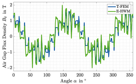
Figure 5.
Simulated air gap flux density of an IM with non-linear stator and rotor magnetic material properties using the T-FEM and E-HWM.
2.4. Numerical Models Based on the Finite Element Method
The analytical models of the FWM, HWM, and E-HWM of the IM are limited in terms of the value range and level of detail of the effects that can be modeled. Effects such as ferromagnetic saturation, induced eddy currents, and a location-dependent air gap reluctance can only be described in a limited and simplified way, as can be seen in the model descriptions. Others, such as cut edge effects [13] or geometry- or motion-dependent phenomena, cannot be modeled at all [14]. An extension of the range of values and level of detail of machine modeling is offered by numerical models. However, the higher level of detail is accompanied by an increase in computational effort. In this paper, the TH-FEM and T-FEM are used and briefly explained in the following. In both cases, a 2D model is used with a current excitation in the form of a specified current density in the stator slots.
2.4.1. Mathematical Description of the FEM
In the FE models of this paper, a magnetoquasistatic formulation over the magnetic vector potential is considered. From the Maxwell equations the parabolic partial differential equation
the reluctance , the conductivity , and the injected stator current density can be derived [14]. A discretization of the magnetoquasistatic formulation in (17) applying the weighted-residual method, which is necessary for the FEM, leads to the weak vector potential formulation
with being weighting functions. The magnetic vector potential is thereby divided into a finite sum of shape functions , and thus is described by its degrees of freedom [14]. Using Galerkin’s method [14], which prescribes , by transformations based on integral theorems and boundary conditions of the solution space, the system of equations and the resulting matrix notation can be expressed as [15]
Here is called stiffness matrix, is called mass matrix, and is called load vector. From this system, the degrees of freedom of the magnetic vector potential and from it the flux density distribution in the machine can be determined.
2.4.2. Time Harmonic Finite Element Model
In the TH-FEM, the time courses of physical quantities are simplified as sinusoidal and can therefore be described by complex phasors [14]
This has the advantage that the time derivative passes into a multiplication by . The differential equation from (19b) thus transforms into the linear system of equations
which can be solved with low computational effort. The disadvantage of the time-harmonic simulation is the underlying assumption that no time harmonics with an order greater than one exist, which is why in particular the accuracy of the calculated iron losses decreases compared with the T-FEM [16].
Slip Transformation
Since the linear equation system (21) simulates the stator frequency in the entire solution domain, the lower frequency in the rotor is not considered. This can be accounted for by a slip transformation [17,18]. For this, the conductivity of the cage is scaled with the slip s, which changes the mass matrix for rotor nodes such that the lower rotor frequency is considered in the induction effect.
Non Linear Material Properties
To consider the non-linear material behavior of the stator and rotor laminations, an iterative procedure is used in the field solution. For this purpose, the successive substitution approach or the Newton method can be used.
2.5. Transient Finite Element Model
The transient simulation solves the differential Equation (19b) for discrete time steps within a time interval considering the field solution of the previous time step and the motion of the rotor. Due to the discretization, the time derivative can be described as the difference quotient with the time difference between two time steps. From this the linear equation system results in
which must be solved for each time step [14]. The corresponding rotor position follows from the Newton equation of motion
with the moment of inertia J of the rotating body. This equation is also discretized in time, with the torque T updated for each time step based on the calculated field solution. By solving the differential equation in the time domain, temporal harmonics in particular are modeled, which allows a more detailed view of the machine behavior. Since the Shannon sampling theorem prescribes a sampling frequency greater than or equal to for physical consideration of a given frequency f [19], the time difference between each time step must be small enough to consider the higher order harmonics, but the total time interval large enough for consideration of the low frequencies in the rotor. This, in combination with the required transient time of the vector potential solution, leads to a high calculation effort of the transient Finite Element (FE) simulation. Faster transient is made possible by a hybrid approach via estimation of a starting solution from an open-circuit simulation [20].
In Figure 6 the simulated magnetic flux density of an exemplary IM at an saturated operating point is shown. In Figure 6a the simulation was conducted using the TH-FEM and in Figure 6b using the T-FEM. The simulation results show quite similar field characteristics.
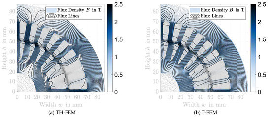
Figure 6.
Simulated magnetic flux density and isolines for an exemplary IM.
2.6. Used Iron Loss Model
The IEM-5 parameter formula is used to calculate the iron losses in each model. It is based on the Bertotti model and adds an additional term considering the non-linear material behavior [21]. The IEM-formula to calculate the iron loss density is given by:
where are the hysteresis, eddy current, and excess loss factors, and are loss parameters describing the non-linear saturation losses, f the frequency, and the amplitude of the magnetic flux density for the given frequency. In the numerical models, the iron loss densities are calculated element by element and weighted by the element area. The summation of the iron loss densities over all elements and multiplication by the iron length then results in the iron losses. In the analytical models, the iron loss densities are calculated for the stator and rotor yokes and teeth respectively with the calculated mean tooth and yoke flux densities. Multiplication by the yoke and teeth mass then also results in the value of the iron losses.
3. Model Selection Approach
The four-step generic procedure of the approach for model selection is shown in Figure 7. The problem definition is based on four input variables. These describe the searched output quantities, the effects to be investigated are whose influence on the output quantities is to be modeled, and the respective required precision, i.e., the problem-specific level of detail. Since the precision of the models depends on the operating point, a selection of the operating points to be considered is also necessary. The problem-specific output quantities to be considered define the electromagnetic coupling quantities for a coupled model. Analogously, the effects to be studied describe the external coupling variables. By means of this problem definition, suitable models can be derived on the basis of the value ranges and levels of detail of the available models and simulation methods, respectively. From the consideration of the value range the possible models follow, which represent all output quantities and effects and can model an influence of the output quantities by the effects. For the possible models, the required level of detail is examined in the following step and the suitable models that meet all requirements are derived from this. From these, the one with the lowest computational effort is selected.
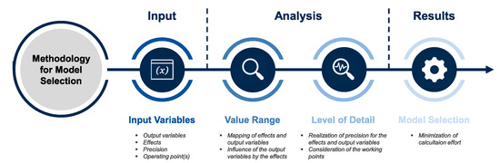
Figure 7.
Process of the approach for the model selection.
One possibility to characterize the range of values and the level of detail of the models are tables, which contain entries for possible output quantities and effects, separated by the available models. The value range table contains a reference to the general ability of the models to describe the output quantities and effects, whereas the level of detail table contains the respective precision. The precision can be given in relation to a reference model, if quantifiable. Alternatively, qualitative scales can be used to describe precision. It is important to have a stringent procedure for the definition of these precisions in order to allow a future consideration of further effects and to make them comparable. Another possibility to describe the range of values and the level of detail, e.g. to consider geometry and material effects, is given by sensitivity analyses, where the parameters to be investigated are slightly varied and it is checked whether the models represent an influence of the parameters on the searched output quantities. Precision is again defined by a reference model. The characterization of the solution effort of the models is done via the number of the respective degrees of freedom since the computation time depends on computer-specific parameters such as the clock speed, the number of cores and the main memory and thus cannot be generalized. In this paper, the described approach for the model selection is presented using the example of an IM. An automated implementation allows finding the most suitable problem-specific model based on the four problem-defining input variables. In the following, the sensitivity analysis used in the selection process and the four steps of the model selection process are presented.
3.1. Sensitivity Analysis
The influence of changes in geometry and material parameters on physical quantities as well as temporal and spatial characteristics is investigated and quantified by means of sensitivity analyses. In the case of coupling one of the presented electromagnetic machine models with another, for example structural dynamic or thermal model, they also provide information about the required accuracy of the coupled model, since the latter does not have to have an influence on machine parameters to which the electromagnetic model is not sensitive.
The starting point of the sensitivity analysis for the IM is a reference geometry. Based on this, a second, slightly modified machine geometry is generated, depending on the geometry or material parameter to be investigated. For this, the parameter is changed by a user defined factor . In this case, too small a change leads to numerical instabilities, and too large changes possibly lead to inconsistent machine geometries. If the sensitivity to a geometry parameter is to be investigated, it is also necessary to consider the influence of this parameter on other geometry variables. For example, if the air gap width is changed, the stator or rotor diameter must also be adjusted. These influences are described via a correlation matrix, which describes for each possible variable geometry parameter which other geometry parameters must also be changed. Subsequently, the machine models are simulated for both geometries and the output quantities are compared. In this work, a T-FEM simulation is not performed in the context of the sensitivity analysis due to the high computational effort associated with it. Instead, the same results are assigned to the T-FEM as to the TH-FEM, since the value ranges and levels of detail are very similar due to analogous procedures in meshing. The following findings can be derived from the comparison of the output quantities of both geometries:
- 1.
- Sensitivity: For each of the models considered in the sensitivity analysis, it can be stated separately for all physical quantities whether they are sensitive to the geometry or material parameter under investigation.
- 2.
- Influence on Harmonics: The influence of the parameter to be examined on the temporal and spatial courses can be described on the basis of the change of the respective harmonic orders of the FFT spectrum. This influence can be recorded qualitatively, but can also be normalized in relation to the largest change of the occurring orders and thus quantified. In this way, the harmonics whose relative change is the greatest can be recorded in particular.
- 3.
- Elasticity: The elasticity describes the ratio of the change of an output quantity, related to the change of the input quantity and therefore results in the case of the sensitivity analysis for a physical quantity towhere describes the relative change of the physical quantity between the two simulated machine models. This allows us to capture, for each model, how much a certain quantity changes when the parameter under investigation is modified.
- 4.
- Level of Detail: The description of the level of detail of the detection of a geometry or material change, related to a physical quantity can be done by means of a reference model. For this purpose, the TH-FEM is selected in this work, since it has the highest average precision after the T-FEM. The degree of detail of a physical quantity, therefore, follows from the relative deviation of the elasticity of the model under consideration from the elasticity of the TH-FEM.
3.2. Input Variables
Possible output quantities of the IM to be investigated are physical quantities such as torque and losses, but also temporal and spatial flux density and torque characteristics. The effects considered in this work include saturation phenomena, harmonics, and other physical effects, but also geometry and material effects as well as dynamic processes. A geometric effect is the change in a geometric quantity, such as the air gap width or tooth width. A material effect is the change of a material property due to external influences such as temperature.
3.3. Analysis of the Value Range and Degrees of Freedom
In the first step, the range of values of the described models is considered. Here, it is investigated for all output quantities and effects whether these can be represented by the value range of the individual models. When considering geometry or material effects, each of the selected output quantities must be influenced by at least one of these effects. The characterization of the value range of the IM is done by means of a table for the output quantities and physical effects and by means of the sensitivity analysis for geometry or material effects. The value range is analyzed in terms of spatial and temporal resolution, the number of degrees of freedom, physical effects, dynamic processes, and physical quantities for the five models presented. Here, for the FE simulations, the degrees of freedom are composed of the number of operating points, the nodes in the mesh, the iterations to account for saturation, and the transient steps. For the HWM, the degrees of freedom are also described by the number of operating points and, in addition, by the stator and rotor orders considered and the Fourier coefficients of the stator and rotor permeance functions. In the E-HWM, the iterations for updating the rotor current are added. The number of degrees of freedom in the FWM is composed only of the simulated stator flux linkages and the operating points.
3.4. Analysis of the Level of Detail
The procedure for characterizing the level of detail is analogous to that for characterizing the range of values via tables and sensitivity analysis. The tables contain precision values of the different physical output parameters and physical effects for linear and non-linear operating points of an exemplary machine in the given power range. The quantification of the precision values of the physical output parameters and effects is performed on the basis of individual categories. These are subdivided as follows:
- Physical Values: For the physical output quantities, such as ohmic losses, and iron losses, the simulation results of the T-FEM is used as a reference. The relative deviations from the results of the T-FEM are determined for exemplary operating points in the linear and non-linear range.
- Temporal and Spatial Characteristic: The precision of temporal and spatial characteristic, such as the magnetic flux density in the stator tooth over time or the magnetic air gap flux over time or position, is determined with reference to the simulation results of the T-FEM. For each characteristic, an exemplary operating point in the linear range and one in saturation are analyzed. The analysis is performed on the basis of the frequency spectrum of the considered quantity. Spatial characteristics, such as the spatial characteristic of the air gap flux density, are decomposed into their spectral components using the Fast Fourier Transformation (FFT) with a rectangular window. The level of detail is then separated into three subcategories. The precision of the fundamental wave, the precision of the harmonic amplitudes, and the precision of the occurring frequency orders. The slip dependence of an operating point during the operation of the IM leads to the fact that frequency components occur in the time variables which do not correspond to an integer multiple of the fundamental frequency. The use of a rectangular window in the FFT therefore leads to large spectral leakage. Therefore, a window function is used for the temporal quantities, which reduces the spectral leakage. A suitable window function is the Hann window. Figure 8a shows an example of the temporal course of the air gap flux density simulated by means of two different models at a particular position in the air gap. In Figure 8b the frequency spectra are plotted by means of a FFT with a rectangular window and by means of a FFT with a Hann window. To determine the level of detail, the output signal of the FFT with the Hann window of the reference signal as well as that of the comparison signal are analyzed for their local maxima. From the local maxima which are larger than a certain threshold value, the level of detail of the fundamental, the amplitudes of the harmonics and the occurring frequencies are then determined, as in the case of the location-dependent characteristics. In Figure 8b the maxima used to analyze the level of detail are marked with numbers.
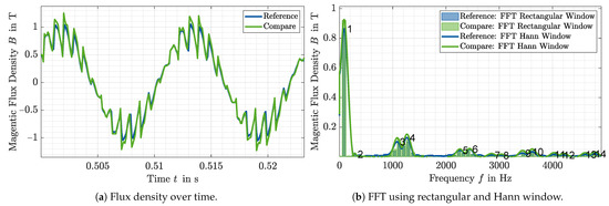 Figure 8. Magnetic air gap flux density simulated by two different models.
 - Physical Effects and Dynamic Processes: Since the level of detail of physical effects and dynamic processes, such as saturation, skin effect, or cutting edge effects, cannot be considered separately from other quantities, these precision are defined using a subjective point scale from one to ten, where one describes a very high precision and ten a very low precision.
The level of detail is analyzed for all output quantities and effects and matched with the required level of detail. The affiliation of an operating point to the linear and non-linear operating range of the machine is thereby determined on the basis of the FWM. The influence of geometry and material effects to be considered must achieve the required precision for each individual influenced output variable.
3.5. Model Selection
Based on the results of the value range analysis and the level of detail analysis, the model with the lowest degree of freedom is then selected from all suitable models. This promises the lowest computational effort and thus the most efficient calculation for the precision requirements. If a working point matrix is considered in the model selection process, the selection of possible models is done analogously based on the range of values. For the resulting models, the precision of the output quantities and effects to be examined are considered in each working point. The selection of the most suitable machine model can then be made using two procedures. One option is to consider those models that have the required level of detail at all operating points. From these, the one with the lowest computational effort is then derived. An alternative is a operating point specific model selection by means of a Branch and Bound optimization, on the basis of which different models can be assigned to different operating points, so that the required level of detail is achieved at each point, but the overall solution effort is minimized.
4. Approach for Parameter Selection
Mathematical optimization algorithms are gaining importance for the design, revision, and optimization of electrical machines. The optimization parameters in the context of such machine optimizations represent those geometry and material parameters that are varied during the optimization procedure in order to find a better solution. These parameters should therefore cover a high degree of freedom of the geometry. However, as the number of optimization parameters increases, so does the search space and the associated solution effort. For this reason, it is advisable to select those geometry parameters that have the greatest influence on the searched output quantities but have the lowest degree of redundancy among themselves. The parameter selection approach presented in this paper describes the selection of such parameters as a methodical procedure. The generic three-step procedure of parameter selection is shown in Figure 9. The process of the parameter selection is problem-specific and is also influenced by the selected system model, which follows from the approach for the model selection. In the context of the optimization environment, the output quantities and effects to be considered in the model selection describe those variables that influence the decision parameters of the optimization problem. The input variables for the problem definition of the parameter selection describe on the one hand the resulting model and the output quantities already described for the methodology for the model selection, but also those problem variables which come into question as optimization parameters. In addition, a selection of the number of parameters to be determined is required, which defines the degrees of freedom and thus the accuracy of the optimization environment, but also describes the required solution effort.
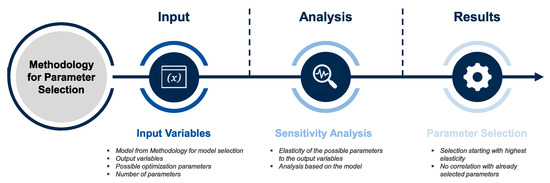
Figure 9.
Process of the approach for the parameter selection.
Based on these input variables, a sensitivity analysis is performed for each possible optimization parameter using the model resulting from the model selection approach. Here, the elasticities of the output quantities relevant to the optimization are examined so that the possible optimization parameters can be sorted based on their elasticity. This identifies those parameters that have the greatest possible influence on the optimization problem, minimizing the global optimum in particular, since this correlates negatively with the elasticity of the optimization parameters. From the sorting of the optimization parameters, starting with the highest elasticity, the given number of parameters can be selected. For each new optimization parameter to be added, the correlation with already selected parameters must be checked, since the individual optimization variables must be independent of each other and must not influence each other. Otherwise, contradictory solutions may result. The optimization parameters resulting from the parameter selection procedure serve as input variables of an optimization environment. Here, a problem-specific, experience-based selection of upper and lower bounds of the parameters is important to reduce the size of the solution space and thus the computational effort. A multi-step optimization environment for the design of an IM using the model and parameter selection procedure presented here is given in [3].
5. Application Example
The model selection procedure is exemplary applied to a multiphysics weakly coupled simulation in this work. The weakly coupled simulation consists of an electromagnetic and a thermal model of an exemplary IM. The electromagnetic model determines the actual temperature-dependent ohmic and iron losses of the IM at different stator winding and rotor cage temperatures. The calculated losses are the input parameters of the thermal model. The thermal model is then used to update the machine temperatures and return them to the electromagnetic model, resulting in a change of the material conductivities. The electromagnetic model to be used is selected by applying the presented approach of model selection. For the thermal model, an implementation in MATLAB® is used, which is based on the Lumped Parameter Thermal Network (LPTN) model of Motor-CAD®. The resulting simulated temperature curves are compared with measured results of the same machine at the same operating point. The use of the parameter selection in combination with the model selection is investigated in [3] using a multi-stage optimization of the design of an IM.
5.1. Exemplary Induction Machine
The exemplary IM is an aluminum die-cast squirrel cage IM. The IM is used as a traction drive in an electrical vehicle. The machine, the cross-sectional area of the stator and rotor and important geometrical and electrical parameters are given in Figure 10. The studied IM delivers a S2 power of and is equipped with a forced air cooling in the housing. The temperature measurement of the IM was performed on a test bench. The test bench setup is described in [22]. Seven temperature sensors were used to measure the average temperature of the stator winding. These were placed at different positions within the winding.
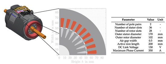
Figure 10.
Cross section and parameter of the exemplary IM.
The rotor temperature measurement was performed using a non-contact infrared (IR) sensor. The temperature was measured at the short-circuit ring of the squirrel-cage. To achieve a high emissivity of the short-circuit ring, it was painted black [23]. The validation of the IR temperature measurement was performed according to the procedure described in [23].
5.2. Thermal Model
An LPTN model of the IM was used as the thermal model. This was built in Motor CAD using the geometry and winding data of the exemplary machine. The LPTN created by Motor-CAD® was extracted and imported into MATLAB®. The thermal parameters and the LPTN of the machine are explained in [24]. The LPTN is solved in Matlab using the modified nodal potential analysis and the Backward Euler method.
Two options can be used to calculate the electromagnetic losses used as input for the thermal simulation. Both options are equivalent in their results. First, in each step where the losses are updated, the electromagnetic model can be calculated with the actual temperatures of the stator winding and the rotor cage. This implies a high computational effort, especially for the numerical models, since the FE simulation must be performed at each step. On the other hand, for a given stator winding and rotor cage temperature, the machine can first be calculated with the selected model and the influences of the temperature changes on the losses can be determined using the scaling laws of IM described in [8,22,25,26]. This reduces the computational effort while maintaining the quality of the calculated losses, as shown in [8,22,25,26].
5.3. Model Selection Approach
The selection of the electromagnetic simulation model of the IM to be used for the described field of application of a coupled electromagnetic-thermal operating point simulation is performed automatically with the presented approach of the model selection. The output quantities and effects to be investigated to describe the problem and the required levels of detail are shown in Table 1. A required level of detail of, for example, means a maximum permissible deviation of from the T-FEM. The required level of detail of the ohmic and stator and rotor losses is obtained assuming a measurement deviation of and a deviation of the electromagnetic reference model, the transient FEM, of . The level of detail of the iron loss components was chosen to be because they have lower losses compared to the ohmic losses at the considered operating point. The required level of detail of the saturation was chosen to be 5 on the subjective point scale, which corresponds to the middle value of the scale. A saturated point in the efficiency maximum of the machine is selected as the operating point to be investigated. With a speed of and a torque of , this lies in the limit between the base speed and the field weakening range of the IM.

Table 1.
Required level of detail of the output quantities and effects of the electromagnetic model.
The model resulting from the procedure, which can represent both the range of values and the required levels of detail, is the E-HWM. The TH-FEM and T-FEM also meet the desired levels of detail, but were not chosen due to the higher degrees of freedom and associated higher computational effort.
5.4. Simulation Results
Using the determined electromagnetic E-HWM, the thermal behavior of the machine is simulated by means of the coupled simulation at the given operating point of and . The simulated and measured temperature of the stator winding and the rotor cage are shown in Figure 11. The stator winding temperature has a maximum deviation of and , respectively, with respect to the measured temperatures during the heat-up phase. The rotor cage temperature shows a deviation of and respectively. These values are therefore within the required level of detail of the losses. For comparison, the simulation is also performed with T-FEM, which has a higher level of detail than the E-HWM, and the FWM, which has a lower level of detail. The results are also plotted in Figure 11. The maximum deviation related to the measurements of the stator winding temperature for the simulation using the T-FEM is and , respectively, and that of the rotor cage temperature is and , respectively. The deviations of the simulations using the FWM are above in both temperatures.
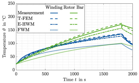
Figure 11.
Simulated and measured stator winding and rotor bar temperature of the exemplary IM using the T-FEM, the E-HWM, and FWM.
6. Discussion
The model and parameter selection approaches presented in this paper are based on the analysis of different analytical and numerical models of an exemplary IM for a given power, torque, and speed range. The analysis is performed at certain operating points and the models are evaluated in terms of their value ranges and levels of detail. The model and parameter selection approaches can then be applied to problems requiring simulations of IM in a similar power, torque, and speed range and with similar geometric dimensions.
In an example simulation of the thermal behavior of an IM the model selection approach is used to determine the most appropriate electromagnetic machine model. The results of this application example show that the model selection approach is suitable for methodically determining the most suitable and computationally efficient model for given requirements in terms of value range and level of detail. Thus, it is an efficient tool for the characterization and methodological analysis of models, especially when selecting one of several models with many different output quantities, effects, and parameters.
The parameter selection procedure provides an approach to identify machine parameters that have a high impact on the defined target variable. This procedure lends itself to the selection of optimization parameters in machine design optimizations as presented in [3].
Author Contributions
Conceptualization, M.N. and A.K.; methodology, M.N. and A.K.; software, M.N. and A.K.; validation, M.N.; formal analysis, M.N.; investigation, M.N. and A.K.; writing—original draft preparation, M.N.; writing—review and editing, M.N., A.K. and K.H.; visualization, M.N. and A.K.; supervision, K.H. All authors have read and agreed to the published version of the manuscript.
Funding
This research received no external funding.
Institutional Review Board Statement
Not applicable.
Informed Consent Statement
Not applicable.
Conflicts of Interest
The authors declare no conflict of interest.
Abbreviations
The following abbreviations are used in this manuscript:
| ECD | Equivalent Circuit Diagram |
| E-HWM | Extended Harmonic Wave Model |
| FE | Finite Element |
| FWM | Finite Element Model |
| FFT | Fast Fourier Transformation |
| FWM | Fundamental Wave Model |
| HWM | Harmonic Wave Model |
| IM | Induction Machine |
| IR | Infrared |
| LPTN | Lumped Parameter Thermal Network |
| MMF | Magnetomotive Force |
| NVH | Noise Vibration Harshness |
| T-FEM | Transient Finite Element Model |
| TH-FEM | Time Harmonic Finite Element Model |
References
- Zienkiewicz, O.C.; Chan, A.H.C. Coupled Problems and Their Numerical Solution. In Advances in Computational Nonlinear Mechanics; Springer: Vienna, Austria, 1989; Volume 300, pp. 139–176. [Google Scholar] [CrossRef]
- Nell, M.; Leuning, N.; Mönninghoff, S.; Groschup, B.; Müller, F.; Karthaus, J.; Jaeger, M.; Schröder, M.; Hameyer, K. Complete and Accurate Modular Numerical Computation Scheme for Multi–Coupled Electric Drive Systems. IET Sci. Meas. Technol. 2020, 14, 259–271. [Google Scholar] [CrossRef]
- Nell, M.; Kubin, A.; Hameyer, K. Multi-Stage Optimization of Induction Machines Using Methods for Model and Parameter Selection. Energies 2021, 14, 5537. [Google Scholar] [CrossRef]
- Oberretl, K. Allgemeine Oberfeldtheorie für ein- und dreiphasige Asynchron- und Linearmotoren mit Käfig unter Berücksichtigung der mehrfachen Ankerrückwirkung und der Nutöffnungen. Teil I: Theorie und Berechnungsverfahren. Arch. Elektrotechnik 1993, 76, 111–120. [Google Scholar] [CrossRef]
- Oberretl, K. Allgemeine Oberfeldtheorie für ein- und dreiphasige Asynchron- und Linearmotoren mit Käfig unter Berücksichtigung der mehrfachen Ankerrückwirkung und der Nutöffnungen. Teil II: Resultate, Vergleich mit Messungen. Arch. Elektrotechnik 1993, 76, 201–212. [Google Scholar] [CrossRef]
- Oberretl, K. Losses, Torques and Magnetic Noise in Induction Motors with Static Converter Supply, Taking Multiple Armature Reaction and Slot Openings into Account. IET Electr. Power Appl. 2007, 1, 517–531. [Google Scholar] [CrossRef]
- Binder, A. Elektrische Maschinen und Antriebe: Grundlagen, Betriebsverhalten; Springer: Berlin/Heidelberg, Germany, 2012. [Google Scholar] [CrossRef]
- Nell, M.; Lenz, J.; Hameyer, K. Scaling Laws for the FE Solutions of Induction Machines. Arch. Electr. Eng. 2019, 68, 677–695. [Google Scholar] [CrossRef]
- Oberretl, K. Die Oberfeldtheorie des Käfigmotors unter Berücksichtigung der durch die Ankerrückwirkung verursachten Statoroberströme und der parallelen Wicklungszweige. Arch. Elektrotechnik 1965, 49, 343–364. [Google Scholar] [CrossRef]
- Stoyanov, L.; Lazarov, V.; Zarkov, Z.; Popov, E. Influence of Skin Effect on Stator Windings Resistance of AC Machines for Electric Drives. In Proceedings of the 16th Conference on Electrical Machines, Drives and Power Systems (ELMA), Varna, Bulgaria, 6–8 June 2019; pp. 1–6. [Google Scholar] [CrossRef]
- Oberretl, K. Einseitiger Linearmotor mit Käfig im Sekundärteil. Arch. Elektrotechnik 1974, 56, 305–319. [Google Scholar] [CrossRef]
- Zhu, Z.Q.; Howe, D. Instantaneous Magnetic Field Distribution in Brushless Permanent Magnet DC Motors. III. Effect of Stator Slotting. IEEE Trans. Magn. 1993, 29, 143–151. [Google Scholar] [CrossRef]
- Elfgen, S.; Steentjes, S.; Bohmer, S.; Franck, D.; Hameyer, K. Influences of Material Degradation Due to Laser Cutting on the Operating Behavior of PMSM Using a Continuous Local Material Model. IEEE Trans. Ind. Appl. 2017, 53, 1978–1984. [Google Scholar] [CrossRef]
- Hameyer, K.; Belmans, R. Numerical Modelling and Design of Electrical Machines and Devices. In Advances in Electrical and Electronic Engineering; WIT Press: Southampton, UK, 1999; Volume 1. [Google Scholar]
- Schöps, S.; De Gersem, H.; Weiland, T. Winding Functions in Transient Magnetoquasistatic Field-Circuit Coupled Simulations. COMPEL Int. J. Comput. Math. Electr. Electron. Eng. 2013, 32, 2063–2083. [Google Scholar] [CrossRef]
- Vassent, E.; Meunier, G.; Foggia, A. Simulation of Induction Machines Using Complex Magnetodynamic Finite Element Method Coupled with the Circuit Equations. IEEE Trans. Magn. 1991, 27, 4246–4249. [Google Scholar] [CrossRef]
- De Gersem, H.; Hameyer, K. Air-Gap Flux Splitting for the Time-Harmonic Finite-Element Simulation of Single-Phase Induction Machines. IEEE Trans. Magn. 2002, 38, 1221–1224. [Google Scholar] [CrossRef]
- De Geserm, H.; Mertens, R.; Kay, H. Comparison of time-harmonic and transient finite element models for asynchronous machines. In Proceedings of the Internationel Conference on Electrical Machines (ICEM00), Espoo, Finland, 28–30 August 2000; Volume 1, pp. 66–70. [Google Scholar]
- Shannon, C.E. A Mathematical Theory of Communication. Bell Syst. Tech. J. 1948, 27, 379–423. [Google Scholar] [CrossRef] [Green Version]
- von Pfingsten, G.; Nell, M.; Hameyer, K. Hybrid Simulation Approaches for Induction Machine Calculation. COMPEL—Int. J. Comput. Math. Electr. Electron. Eng. 2018, 37, 1744–1754. [Google Scholar] [CrossRef]
- Steentjes, S.; von Pfingsten, G.; Hombitzer, M.; Hameyer, K. Iron-Loss Model With Consideration of Minor Loops Applied to FE-Simulations of Electrical Machines. IEEE Trans. Magn. 2013, 49, 3945–3948. [Google Scholar] [CrossRef]
- Nell, M.; Groschup, B.; Hameyer, K. Using Scaled Fe Solutions for an Efficient Coupled Electromagnetic—Thermal Induction Machine Model. COMPEL—Int. J. Comput. Math. Electr. Electron. Eng. 2021, 40, 267–279. [Google Scholar] [CrossRef]
- von Pfingsten, G.; Steentjes, S.; Hameyer, K. Operating Point Resolved Loss Calculation Approach in Saturated Induction Machines. IEEE Trans. Ind. Electron. 2017, 64, 2538–2546. [Google Scholar] [CrossRef]
- Groschup, B.; Nell, M.; Pauli, F.; Hameyer, K. Characteristic Thermal Parameters in Electric Motors: Comparison between Induction- and Permanent Magnet Excited Machine. IEEE Trans. Energy Convers. 2021, 36, 2239–2248. [Google Scholar] [CrossRef]
- Nell, M.; Lenz, J.; Hameyer, K. Efficient Numerical Optimization of Induction Machines by Scaled FE Simulations. In Proceedings of the XIII International Conference on Electrical Machines (ICEM), Alexandroupoli, Greece, 3–6 September 2018; pp. 198–204. [Google Scholar] [CrossRef]
- Nell, M.; Groschup, B.; Hameyer, K. Efficient Coupled Electromagnetic-Thermal Induction Machine Model Using Scaled FE-Solutions. In Proceedings of the 19th International Symposium on Electromagnetic Fields in Mechatronics, Electrical and Electronic Engineering (ISEF), Nancy, France, 29–31 August 2019; pp. 1–2. [Google Scholar] [CrossRef]
Publisher’s Note: MDPI stays neutral with regard to jurisdictional claims in published maps and institutional affiliations. |
© 2021 by the authors. Licensee MDPI, Basel, Switzerland. This article is an open access article distributed under the terms and conditions of the Creative Commons Attribution (CC BY) license (https://creativecommons.org/licenses/by/4.0/).