Model Predictive Control for Efficient Management of Energy Resources in Smart Buildings

Abstract

Efficient management of energy resources is crucial in smart buildings. In this work, model predictive control (MPC) is used to minimize the economic costs of prosumers equipped with production units, energy storage systems, and electric vehicles. To this purpose, the predictive control manages the available energy resources by exploiting future information about energy prices, absorption and production power profiles, and electric vehicle (EV) usage, such as times of departure and arrival and predicted energy consumption. The predictive control is compared with a rule-based technique, herein referred to as a heuristic approach, that acts in an instant-by-instant fashion without considering any future information. The reported results show that the studied predictive approach allows one to achieve charging profiles that adapt to variable operating conditions, aiming at optimal performances in terms of economic cost minimization in time-varying price scenarios, reduction of rms current stresses, and recharging capability of EV batteries. Specifically, unlike the heuristic method, the MPC approach is proven to be capable of efficiently managing the available energy resources to ensure a full recharge of the EV battery during nighttime while always respecting all system constraints. In addition, the proposed control is shown to be capable of keeping the peak power absorption from the grid constrained within set limits, which is a valuable feature in scenarios with widespread adoption of EVs in order to limit the stress on the electrical system.

1. Introduction

The deregulation of the electric power industry has recently become a topic of attention for investors, regulators, and other participants who aim to achieve decarbonization in the energy sector and a more efficient use of energy [1]. In this context, smartgrids allow the enhancement of the efficiency of electricity utilization from the points of generation to the end users, and they enable the participation of prosumers on the demand side. Home nanogrids usually consist of renewable energy sources (RESs) and energy storage systems (ESSs) that can be used to store or release power when needed. Electric vehicles (EVs) using electricity produced by renewable sources appear as a promising solution for a sustainable transportation sector in the near future [2,3,4,5,6]. EVs use rechargeable battery packs to store the energy needed for propulsion. Smart buildings can be equipped with charging points where EV batteries can be recharged, for example, during nighttime [7]. On the other hand, concerns have been raised that are related to the peak power required to allow a proper recharge of EV batteries [4].

In this field, demand response (DR) will play an important role in the coordination of energy production and consumption by prosumers [8,9]. DR programs can be categorized as (i) incentive-based, where measures affect prosumers’ behavior by providing incentives, or (ii) price-based, where electricity price variations are used to induce the prosumers to correspondingly adapt their electricity usage [10,11,12]. Under this latter category, time of use (TOU) and real-time pricing (RTP) are the most commonly adopted approaches to retail pricing [9,13]. With TOU, electricity prices are changed in order to follow the shape of the demand (e.g., higher prices during peak-load periods), while with RTP, prices are modified to follow the trends of the electricity market.

In such a scenario, the flexible and efficient management of prosumers’ energy resources is crucial in order to make DR a win–win solution for both the electrical system and the prosumers. The implementation of an efficient management system can be achieved through the development of advanced control strategies that aim to increase the demand flexibility and to minimize the economic expenditures of prosumers [14]. In this context, model predictive control (MPC) [15,16] represents one of the most promising control methodologies for achieving an efficient management of users’ resources. MPC is an advanced control strategy whose aim is to minimize an objective function over a prediction horizon while always satisfying a set of system constraints; due to its versatility, it has been largely adopted in applications in power systems [17,18,19,20,21,22,23]. For example, in [24], an MPC method was developed for a microgrid equipped with photovoltaic (PV) sources and ESSs while taking both the economic expenditure given by the power exchange with the upstream grid and the battery’s wear cost into account in the objective function. In that work, the results of the MPC were studied with respect to the difference between the purchase and sale prices, but the electricity price was kept constant. Varying electricity prices were considered in [25], in which an energy management system based on MPC was developed and experimentally tested. The experimental infrastructure was located at the FlexElec Laboratory in the University of Nottingham, and it comprised an ESS and PV panels. The target of the MPC was to minimize the electricity bill. In the study, particular attention was given to the economic performance of the predictive control as different parameters were varied, such as the ESS capacity and the PV size. In [26], the economic MPC developed was compared with a simple control method that was implemented in a rule-based manner. The performances of the developed MPC for different price scenarios were investigated in the paper, and it was underlined that, when compared with simple control solutions, the MPC presented advantages with time-varying prices and that such advantages increased as the energy price variability rose.

In this work, the predictive control is used to efficiently manage a home nanogrid equipped with a PV source, an ESS, and a connection to the upstream grid, with the specific task of recharging the battery of an EV while fulfilling all of the operational constraints. A typical scenario that assumes that the EV battery is recharged overnight to take advantage of the lower prices commonly applied by retailers is considered. By exploiting predictions of absorption and generation profiles, energy prices, times of departure and arrival of the EV, and daily EV battery energy consumption, the predictive control manages the available energy resources with a twofold aim:

• Minimizing the economic costs of the system;
• Fully charging the EV battery during nighttime while respecting the maximum exchanged power constraints at the point of connection with the grid.

The MPC is compared with a simple control method called the heuristic approach that, unlike the MPC, manages the system in a rule-based fashion without taking any future information into account. The two control strategies are compared by considering two different perspectives. The first one regards the economic performances of the approaches in two different price scenarios—a flat TOU rate and a steep TOU rate. In this context, the MPC proves to be a better solution than the heuristic approach because it achieves lower economic costs with greater economic savings for the steep TOU rate, which is characterized by a high purchase-price variability. In addition, rms current stresses are reduced thanks to the MPC approach. The second perspective regards the functionality of the control methods: the MPC is capable of fully recharging the EV battery during nighttime in scenarios in which the heuristic method is not. This merit is due to the smart management allowed by the MPC approach, which is shown to be capable of fully exploiting the available resources while still satisfying all system constraints.

The organization of the paper is as follows. In Section 2, the system model of the nanogrid considered is reported. The heuristic approach is described in Section 3. Section 4 describes the proposed energy management system based on MPC. In Section 5, the MPC approach and the heuristic method are compared by considering the economic costs obtained in a seven-day simulation period, while Section 6 proposes a functional comparison between the two control approaches. The conclusions are reported in Section 7.

2. System Model

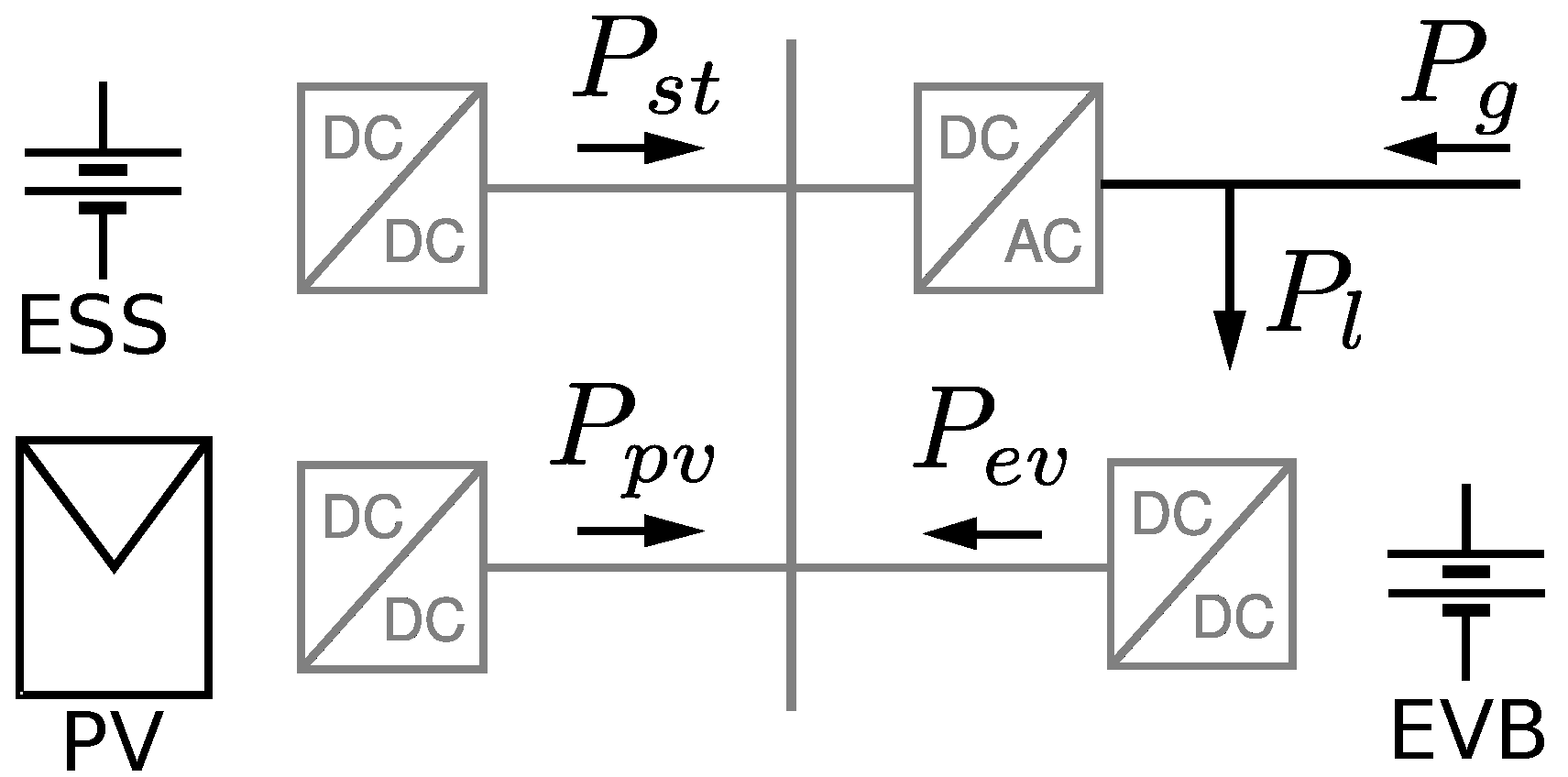
The smart building under consideration is provided with a nanogrid that connects the energy sources and loads, as shown in Figure 1. The nanogrid is composed of:

• Connection with the upstream grid with which the nanogrid exchanges power $P_g$. The maximum power that can be requested from the grid is denoted by $P_{g,max}$, which is assumed to be greater than 0 W.
• Photovoltaic (PV) sources, which generate the output power $P_{pv}$.
• Loads, which absorb power $P_l$.
• An energy storage system (ESS), which generates power $P_{st}$ and has a capacity $E_{st,N}$, maximum discharging power $P_{st,max}$, and maximum charging power $P_{st,min}$. The capacity range of the ESS is given by the closed interval $\left[E_{st,min},E_{st,max}\right]$.
• An electric vehicle battery (EVB), which generates power $P_{ev}$ and has a capacity $E_{ev,N}$. In this paper, $P_{ev}$ is assumed to be non-positive ($P_{ev}\le 0$), i.e., the EVB can not provide power to the other system resources. The closed interval $\left[E_{ev,min},E_{ev,max}\right]$ represents the capacity range of the EVB.

Both the ESS and the EVB are modeled as a dynamic discrete-time system with $\Delta T$ as sampling interval:

$$\begin{array}{c}\hfill \begin{array}{c}\hfill E_{st}^{+}=E_{st}-\Delta T{P}_{st},E_{ev}^{+}=E_{ev}-\Delta T{P}_{ev},\end{array}\end{array}$$

(1)

where $E_{st}$ and $E_{ev}$ are the stored energy in the ESS and EVB, respectively, with superscript ${}^{+}$ referring to the value of the variable at the following time.

The model of the system with $P_{st}$ and $P_{ev}$ as inputs can be summarized in the following discrete-time equation:

$$\begin{array}{c}\hfill \begin{array}{c}\hfill \left[\begin{array}{c}{E}_{st}^{+}\\ E_{ev}^{+}\end{array}\right]=\left[\begin{array}{cc}1& 0\\ 0& 1\end{array}\right]\left[\begin{array}{c}{E}_{st}\\ E_{ev}\end{array}\right]+\left[\begin{array}{cc}-\Delta T& 0\\ 0& -\Delta T\end{array}\right]\left[\begin{array}{c}{P}_{st}\\ P_{ev}\end{array}\right].\end{array}\end{array}$$

(2)

According to Figure 1, the power balance equation of the nanogrid is given in the following:

$$\begin{array}{c}\hfill \begin{array}{c}\hfill P_l=P_{pv}+P_{st}+P_{ev}+P_g.\end{array}\end{array}$$

(3)

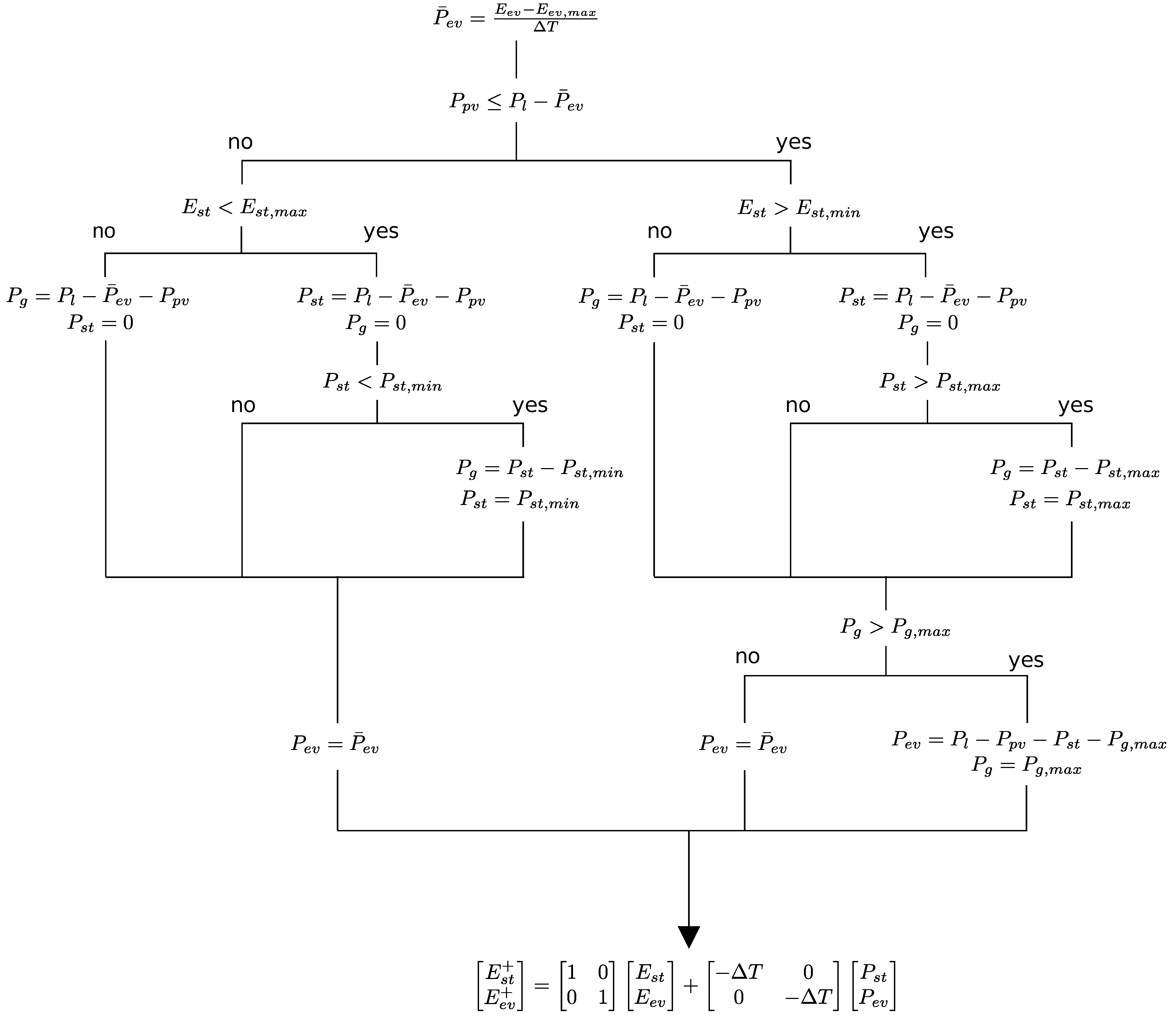
3. Heuristic Approach

In this paper, the proposed MPC strategy is compared with a rule-based technique, which is called the heuristic approach hereinafter.

When the EV is connected to the nanogrid (i.e., during nighttime), the heuristic method devotes all the available resources to the charging process of the EVB; to this purpose, at each time step, given the current value of the battery’s state of charge $E_{ev}$, by exploiting (1), the signal ${\overline{P}}_{ev}$ is computed as:

$$\begin{array}{c}\hfill \begin{array}{c}\hfill {\overline{P}}_{ev}=\frac{E_{ev}-E_{ev,max}}{\Delta T}.\end{array}\end{array}$$

(4)

When the EV is not connected to the nanogrid (i.e., during daytime), signal ${\overline{P}}_{ev}$ becomes:

$$\begin{array}{c}\hfill \begin{array}{c}\hfill {\overline{P}}_{ev}=0\mathrm{W}.\end{array}\end{array}$$

(5)

The heuristic method manages the ESS to achieve $P_g=0$, if possible; at each time step, it compares the values of $P_{pv}$ and $P_l-{\overline{P}}_{ev}$:

• If $P_{pv}\le P_l-{\overline{P}}_{ev}$, the shortage of power is satisfied by the ESS; when the ESS does not have enough power capacity or it is empty, the approach computes the grid power $P_g$ to satisfy the excess demand. Then:

  −

  If $P_g$ is lower than or equal to $P_{g,max}$, the EV charging power is given by:

  $$\begin{array}{c}\hfill \begin{array}{c}\hfill P_{ev}={\overline{P}}_{ev};\end{array}\end{array}$$

  (6)

  −

  If $P_g$ exceeds $P_{g,max}$, the grid power is set to satisfy the upper bound limit:

  $$\begin{array}{c}\hfill \begin{array}{c}\hfill P_g=P_{g,max},\end{array}\end{array}$$

  (7)

  and the resulting EV charging power is yielded by (3):

  $$\begin{array}{c}\hfill \begin{array}{c}\hfill P_{ev}=P_l-P_{pv}-P_{st}-P_g;\end{array}\end{array}$$

  (8)

• If $P_{pv}>P_l-{\overline{P}}_{ev}$, the excess power is stored in the ESS; in case the ESS is full or does not have sufficient power capacity, the unused power is diverted into the grid. As far as the EVB is concerned, because, in this case, the following inequality holds:

  $$\begin{array}{c}\hfill \begin{array}{c}\hfill P_g\le 0<P_{g,max},\end{array}\end{array}$$

  (9)

  the actual power absorbed by the battery is given by:

  $$\begin{array}{c}\hfill \begin{array}{c}\hfill P_{ev}={\overline{P}}_{ev}.\end{array}\end{array}$$

  (10)

It is worth noting that, at each time step, the computed power ${\overline{P}}_{ev}$ is a fictitious signal; the actual EVB charging power $P_{ev}$ is equal to ${\overline{P}}_{ev}$ if $P_g\le P_{g,max}$.

The steps of the heuristic approach are shown in Figure 2.

4. Model Predictive Control

Model predictive control is an advanced model-based control strategy whose aim is to optimize the evolution of a system over a future time span. At each sampling time, the predictive control computes the control signal by minimizing a cost function over a prediction horizon while taking system constraints into account. Only the first input of the signal is applied; then, the model state is updated and the optimization operation is iterated by adopting a receding horizon strategy.

In the proposed energy management system formulation, the MPC exploits future information about the expected power absorption and generation profiles, energy prices, times of departure and arrival of the EV, and daily EVB energy consumption with the aim of:

• Minimizing the overall economic costs of the system;
• Managing the system to achieve a full recharge of the EVB overnight.

In this paper, a particular case is considered in which future information about production and absorption profiles, departure and arrival times of the EV, and daily EVB energy consumption is assumed to be known, as the target is to highlight the advantages that can potentially be obtained by exploiting predictive approaches. Studying how prediction errors may degrade the performance of the MPC procedure will be the target of future work.

4.1. Cost Function

The MPC computes the control inputs that minimize the cost function J over a prediction horizon $N_p$:

$$\begin{array}{c}\hfill \begin{array}{c}\hfill \underset{\{P_{st}\left(k\right),P_{ev}\left(k\right)\}}{min}J=J_e-J_f,\end{array}\end{array}$$

(11)

with

$$\begin{array}{c}\hfill \begin{array}{c}\hfill J_e=\Delta T\sum _{k=1}^{N_p}\left(c_p\left(k\right)\max (P_g\left(k\right),0)+c_s\left(k\right)\min (P_g\left(k\right),0)+c_{ESS}\left|P_{st}\left(k\right)\right|\right),\end{array}\end{array}$$

(12)

and

$$\begin{array}{c}\hfill \begin{array}{c}\hfill J_f=c_f{E}_{st}\left(N_p\right).\end{array}\end{array}$$

(13)

$J_e$ is the economic cost over the prediction horizon and is given by the sum of the following three terms:

• The first term is the cost of purchasing energy; $c_p$ is the purchase price, and is measured in EUR/kWh.
• The second term is the cost of selling energy (this term is negative, resulting in a positive revenue); $c_s$ is the sale price, and is measured in EUR/kWh.
• The third term weighs the degradation of the ESS with the coefficient $c_{ESS}$, which is measured in EUR/kWh and will be defined in Section 4.3. This term considers the economic cost due to the wear of the storage unit.

The term $J_f$ represents an economic value that is proportional to the final state of charge of the ESS in the prediction horizon via the positive coefficient $c_f$, which is measured in EUR/kWh. High values of $c_f$ may lead to a fully charged ESS at the end of the prediction horizon, whilst low values lead to an empty ESS. The best setting of this coefficient depends on the price scenario under consideration and aims to mitigate the effect of a limited prediction horizon on the economic cost.

From (1), the following equation holds:

$$\begin{array}{c}\hfill \begin{array}{c}\hfill E_{st}\left(N_p\right)=E_{st}\left(0\right)-\Delta T\sum _{k=1}^{N_p}{P}_{st}\left(k\right).\end{array}\end{array}$$

(14)

Then, the cost function J can be written as follows:

$$\begin{array}{c}\hfill \begin{array}{c}\hfill J=\Delta T\sum _{k=1}^{N_p}\left(c_p\left(k\right)\max (P_g\left(k\right),0)+c_s\left(k\right)\min (P_g\left(k\right),0)+c_{ESS}\left|P_{st}\left(k\right)\right|+c_f{P}_{st}\left(k\right)\right).\end{array}\end{array}$$

(15)

4.2. System Constraints

The MPC minimizes the cost function in (15) in the prediction horizon under the following constraints for the ESS:

$$\begin{array}{c}\hfill \begin{array}{c}\hfill \begin{array}{c}\hfill \left\{\begin{array}{c}{E}_{st,min}\le E_{st}\le E_{st,max}\hfill \\ P_{st,min}\le P_{st}\le P_{st,max}\hfill \end{array}\right..\end{array}\end{array}\end{array}$$

(16)

Considering the EVB constraints, when the EV is connected to the nanogrid (i.e., during nighttime), the following constraints hold:

$$\begin{array}{c}\hfill \begin{array}{c}\hfill \begin{array}{c}\hfill \left\{\begin{array}{c}{E}_{ev,min}\le E_{ev}\le E_{ev,max}\hfill \\ E_{ev}\left(T_{d,i}\right)=E_{ev,max}\hfill \\ P_{ev}\le 0\hfill \end{array}\right.,\end{array}\end{array}\end{array}$$

(17)

where $T_{d,i}$ refers to the departure time of the EV at the end of the i-th nighttime period; in this way, the MPC procedure ensures, if possible, a full EVB at the departure time. Otherwise, when the EV is not connected to the nanogrid (i.e., during daytime), the following equality constraint holds:

$$\begin{array}{c}\hfill \begin{array}{c}\hfill P_{ev}=0.\end{array}\end{array}$$

(18)

As regards the grid power, the MPC optimizes the system under the following inequality constraint:

$$\begin{array}{c}\hfill \begin{array}{c}\hfill P_g\le P_{g,max}.\end{array}\end{array}$$

(19)

4.3. Estimating the Economic Cost of ESS Wear

In the literature dealing with the economic optimization tasks for ESSs, a term in the cost function is usually added with the aim of preserving the life expectancy of the storage. In this paper, a common approach is adopted that consists of including a term that is proportional to the absolute value of the ESS’s exchanged output power in the cost function [18]. The coefficient $c_{ESS}$ in (15) is defined as the ratio between the ESS price and the total energy throughput bearable by the ESS in its whole usable life:

$$\begin{array}{c}\hfill \begin{array}{c}\hfill c_{ESS}=\frac{C_{ESS}}{2N_{cy}{E}_{st,N}},\end{array}\end{array}$$

(20)

where $C_{ESS}$ is the cost of the ESS, $N_{cy}$ is its expected cycle lifetime, and $E_{st,N}$ is its capacity.

It is worth noting that since the aim of the MPC is to fully charge the EVB during nighttime with the constraint $P_{ev}\le 0$, no EVB degradation cost is included in the cost function (15); the inclusion of a battery degradation cost would not modify the optimization results.

5. Economic Comparison

In this section, the economic performances of the MPC and the heuristic method are compared by considering different price scenarios. The first price scenario considers a TOU tariff with low purchase-price variations, and it is based on rates that are currently available in Italy. The second tariff considers typical Australian TOU rates with a high purchase-price variation between nighttime and daytime.

The nanogrid under consideration is provided with an ESS with a nominal capacity of 13.5 kWh and maximum output power of 4 kW, which corresponds to a commercial size for the considered application [27]; it is assumed that the ESS can be used in the range $\left[E_{st,min},E_{st,max}\right]$, where $E_{st,min}$ and $E_{st,max}$ are equal to 2 and 13.5 kWh, respectively. The ESS is assumed to have an expected lifetime of 5000 cycles and a cost of 7030 EUR, which means that $c_{ESS}=0.0521$ EUR/kWh.

The EV is provided with a battery with a nominal capacity of 42 kWh, which is an average and representative value considering the current storage capacities of EVs of small/medium size [28]. The EVB can be used in the range $\left[E_{ev,min},E_{ev,max}\right]$, where $E_{ev,min}$ and $E_{ev,max}$ are equal to 6 and 42 kWh, respectively. A typical scenario is considered in which the driver leaves home in the morning and returns home in the afternoon or in the evening. The times of departure and arrival of the EV and the corresponding battery energy consumption during the week are reported in

Table 1. The departure and arrival times and EVB energy consumption considered.

Day of the Week	Departures	Arrivals	Energy Consumption
Wednesday	6 a.m.	18 p.m.	10.80 kWh
Thursday	6 a.m.	18 p.m.	7.20 kWh
Friday	6 a.m.	18 p.m.	10.80 kWh
Saturday	7 a.m.	21 p.m.	3.60 kWh
Sunday	7 a.m.	21 p.m.	19.80 kWh
Monday	6 a.m.	18 p.m.	10.80 kWh
Tuesday	6 a.m.	18 p.m.	3.60 kWh

. An average consumption of 28.49 kWh per 100 statute miles is assumed, which is typical for the size of the considered EV, considering a driver traveling, on average, about 33.40 statute miles per day [29]. It is assumed that the EV connects to the nanogrid at the time of arrival.

In the simulations, the model sample time is 60 s, while the control sample time is set to one hour for both the MPC and the heuristic method. The prediction horizon is set to 24 h in the predictive controller; this choice represents a proper trade-off between the reliability of predictions and energy cost minimization; shorter prediction horizons would bring an increase in the economic costs.

The two control procedures are compared in a seven-day simulation period, where the load and PV data refer to an installation of a rated load power of 3 kW and a rated PV generation unit of 4 kW; the average daily energy absorbed by the loads is about 16.15 kWh/day, while the average daily PV energy generated is about 13.26 kWh/day.

5.1. Scenario 1: MPC—Flat Time-of-Use Rate

A TOU retail tariff typically applied in the Italian market is adopted in this scenario [30]; it is characterized by a slightly varying purchase price based on three time intervals: (i) high consumption (midday hours), (ii) low consumption (nighttime), and (iii) weekends. Prices in the second and third intervals usually coincide in the Italian market.

As regards the selling price, in Italy, a state-run net metering scheme for power injections of small generators is employed; excess PV energy is sold at market price, and then, at the end of the year, the prosumer receives a payment based on the injected and absorbed energy [31].

In this price scenario, the coefficient $c_f$ is set to 0.17 EUR/kWh. It was verified that both lower and higher values can bring an increase in the economic cost; with lower values, the controller cannot exploit all of the available PV power to charge the ESS, while with higher values, the discharge of the ESS when demand exceeds production cannot be guaranteed, even in the case of the availability of energy in the ESS.

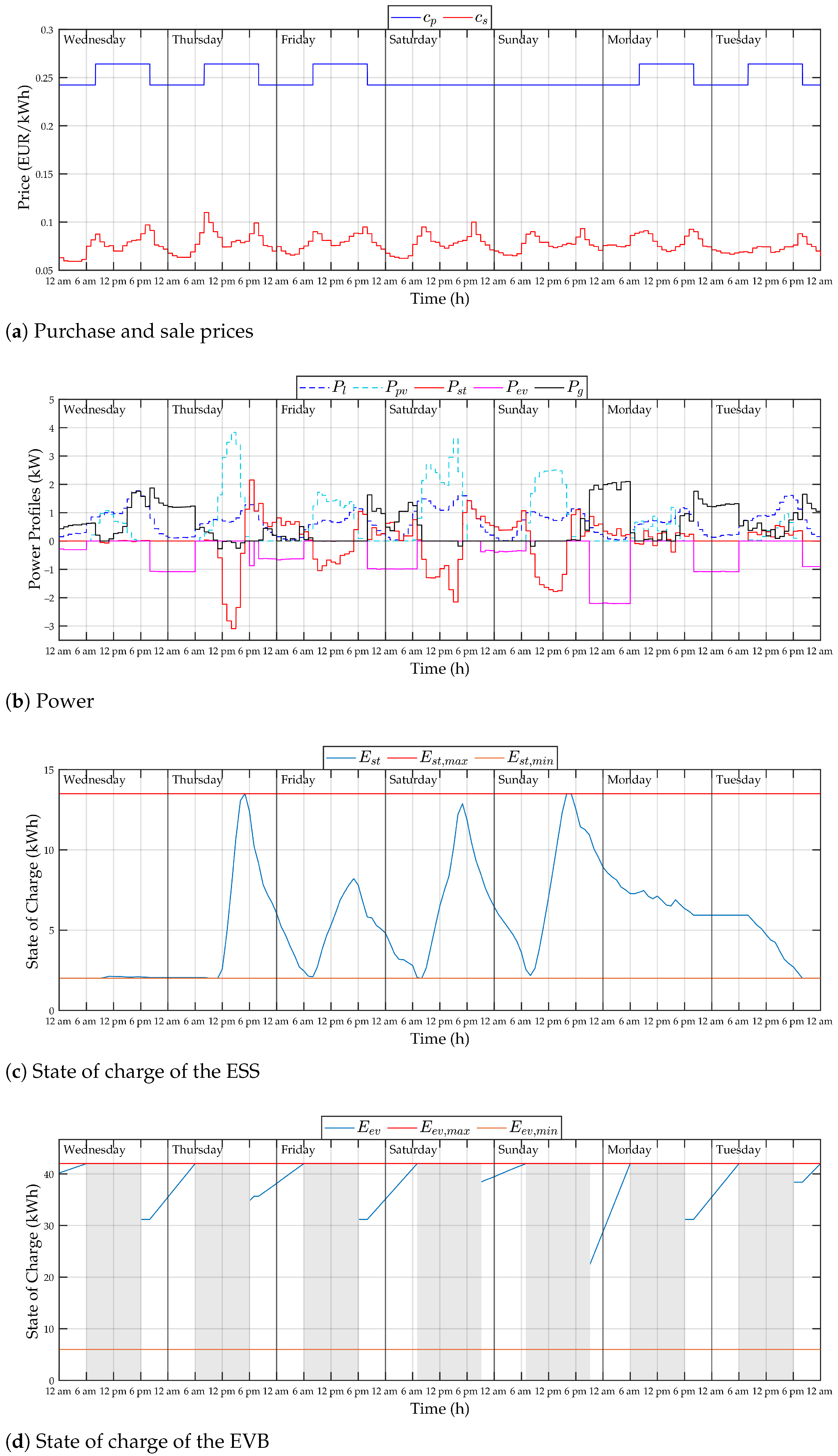
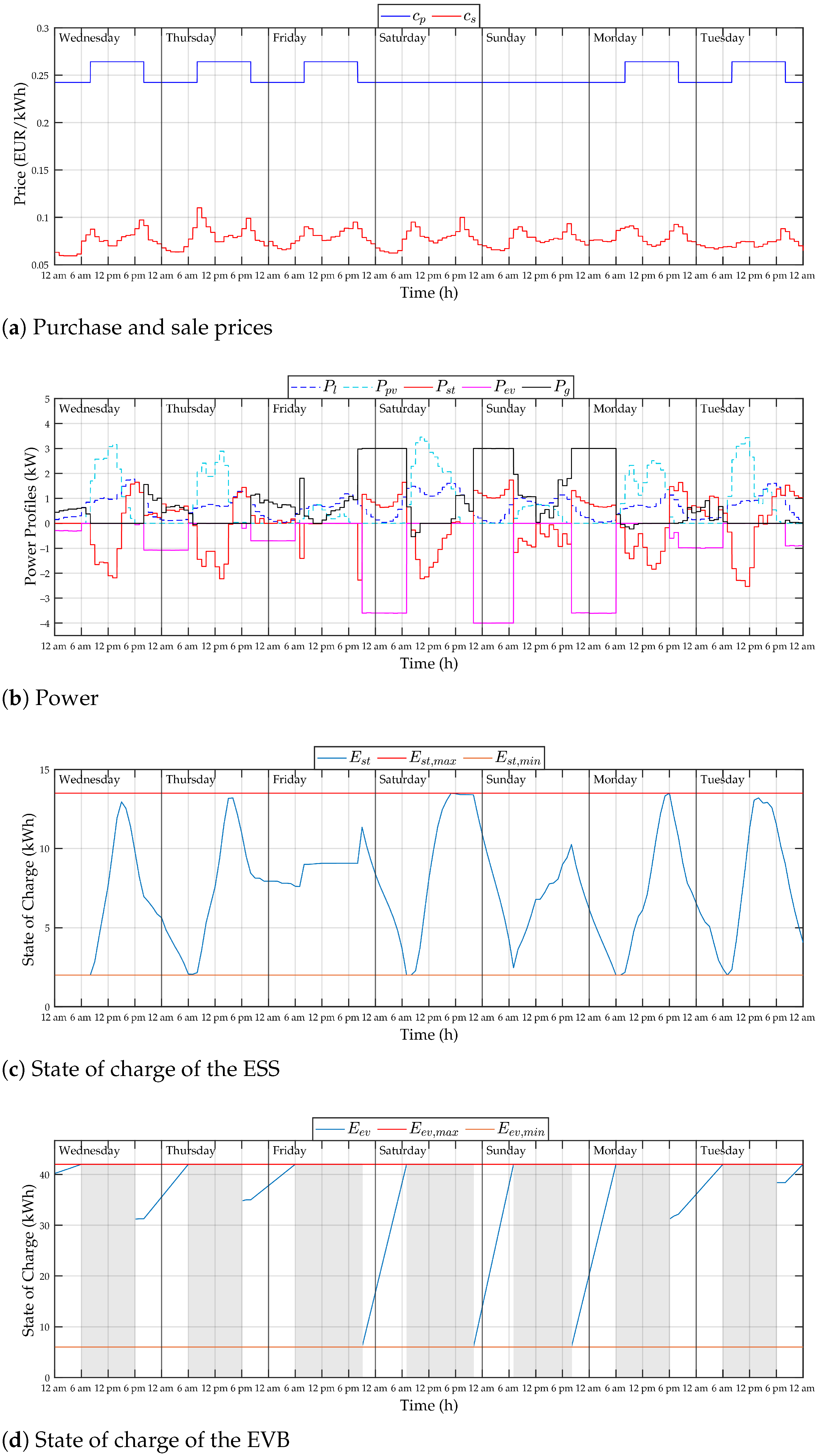
Figure 3 shows the energy prices and the predictive control simulation results. The cost of energy (Figure 3a) is 0.2642 EUR/kWh from 8 a.m. to 8 p.m. and 0.2424 EUR/kWh from 8 p.m. to 8 a.m. on working days, while on the weekend, it is a constant signal that is equal to 0.2424 EUR/kWh. The sale price changes on a daily basis, with small variations. In the simulations, it was assumed that the sale price for the upcoming day is known at 4 p.m.; in case of an unknown sale price at a specific time in the prediction horizon, the controller is fed with an average value based on the three previous days.

Power profiles are given in Figure 3b, while the states of charge of the ESS and the EVB are reported in Figure 3c,d, respectively (in Figure 3d, the time interval in which the EV is not connected to the nanogrid is shaded). It can be observed that that the ESS charges if the production exceeds the load during the daytime, while during the nighttime, power is driven from the ESS to the EVB, if possible (e.g., during the night between Saturday and Sunday); if the ESS cannot provide enough energy to charge the EVB, the predictive control purchases the required energy from the grid during the low-price periods. Notably, the MPC proves to be able to fully charge the EVB by smartly managing available energy resources with minimal economic expenditures.

5.2. Scenario 2: MPC—Steep Time-of-Use Rate

A tariff currently applied in the Australian electricity market is considered in this scenario [32]. It is characterized by a high variability in purchase price based on the following time intervals: (i) peak (midday hours), (ii) shoulders (morning, late evening, and weekend), and (iii) off-peak (nighttime). Furthermore, Australian retailers apply a daily charge between 0.90 and 1.20 AUD/day; in this case, a daily supply charge of 1.10 AUD/day is considered. As regards the selling price, in Australia, a flat rate that varies between 0.09 and 0.12 AUD/kWh is adopted; here, a sale price $c_s$ equal to 0.12 AUD/kWh is applied. In the tests performed, an exchange rate of 0.6 EUR/AUD is considered.

In this price scenario, the coefficient $c_f$ is set to 0.15 EUR/kWh. As described above, both lower and higher values can lead to an increase in the economic cost.

Figure 4 reports the simulation results for the MPC approach. On working days, the purchase price is 0.2376 EUR/kWh from 3 p.m. to 9 p.m. (peak), 0.1295 EUR/kWh from 7 a.m. to 3 p.m. and from 9 p.m. to 10 p.m. (shoulder), and 0.1086 EUR/kWh from 10 p.m. to 7 a.m. (off-peak). On the weekends, it is 0.1295 EUR/kWh from 7 a.m. to 10 p.m. (shoulder) and 0.1086 EUR/kWh from 10 p.m. to 7 a.m. (off-peak). The sale price is a constant signal that is equal to 0.072 EUR/kWh.

Differently from the previous price scenario, on Wednesday, the ESS charges during the off-peak time, thus exploiting the grid with the aim of satisfying the daytime demand during the peak price period, since the ESS is empty at the beginning of the considered period and the controller predicts a lack of generation in the prediction horizon; this is due to the daily purchase price difference, which is higher than $2c_{ESS}$ [26]. It is worth noting that the ESS is used only to satisfy the demand during the peak period of the working days, while on the shoulders and off-peak times, the grid is exploited to satisfy the load and to charge the EVB. Unlike in the previous scenario, there is no power transfer from the ESS to the EVB. This happens because, at the shoulder and off-peak times, the difference between the purchase and selling prices is lower than $2c_{ESS}$; the use of the ESS would increase the economic costs with respect to the solution of exploiting the grid to charge the EVB due to the cost of wear of the storage. Similarly to scenario 1, the MPC buys energy to charge the EVB during the lowest price period (from 10 p.m. to 7 a.m.).

5.3. Simulation with the Heuristic Approach

Figure 5 reports the simulation results for the heuristic method. The same results are achieved for the two price scenarios considered, since the implementation of the algorithm of the heuristic approach does not depend on energy prices. During the daytime, when production exceeds absorption, excess PV power is diverted into the ESS or, if the storage is full, into the grid. Instead, when the PV power is lower than the load, the deficit is satisfied by the ESS or, if empty, by the grid. At the arrival time, the heuristic approach uses all of the available resources to charge the EVB, and then exploits the power provided by the ESS with an upper bound of 4 kW and that of the grid with an upper bound of 3 kW. As seen with the MPC, during the nighttime, the heuristic method is capable of fully recharging the EVB before the next departure time.

5.4. Economic Costs

In this subsection, the performances of the predictive control and the heuristic method are evaluated by comparing the economic costs achieved in the simulations reported above.

The economic costs for the MPC and the heuristic approach in the considered price scenarios are reported in

Table 2. Economic costs in the considered interval of one week.

Control Methodology		Scenario 1: Flat TOU Rate					Scenario 2: Steep TOU Rate
		Purchase	Sale	ESS	Charge	Overall	Purchase	Sale	ESS	Charge	Overall
MPC	(EUR)	22.13	−0.09	4.24	0	26.28	12.53	−1.65	2.74	4.62	18.24
Heuristic approach	(EUR)	22.69	−0.09	4.23	0	26.83	15.68	−0.08	4.23	4.62	24.45

; the overall economic cost consists of the three terms defined in Section 4.1:

• Energy purchase: cost of energy purchase,
• Energy sale: cost of energy sale (this term is negative),
• ESS wear: economic cost due to the wear of the ESS,

as well as the charge, which comes from a fixed daily value of 0.66 EUR/day in Scenario 2, while in Scenario 1, there is no charge.

As far as the overall economic costs are concerned, the economic savings of the MPC compared to the heuristic strategy are 2.05% in Scenario 1 and 25.40% in Scenario 2, rising up to 31.32% if the charge is not considered. The performance of the MPC increases with the increase in the daily price variability. In Scenario 1, which is characterized by a low daily variability of the purchase price, low savings are achieved, while in Scenario 2, much greater savings are achieved due to the high variation in the purchase price.

The MPC proves to be a better solution than the heuristic technique because it obtains lower economic costs by smartly managing available energy resources. Notably, such smart control actions are not possible with techniques that act in an instant manner, such as the heuristic approach considered here. It is worth remarking that the economic advantages obtained increase as the daily price variability rises [26].

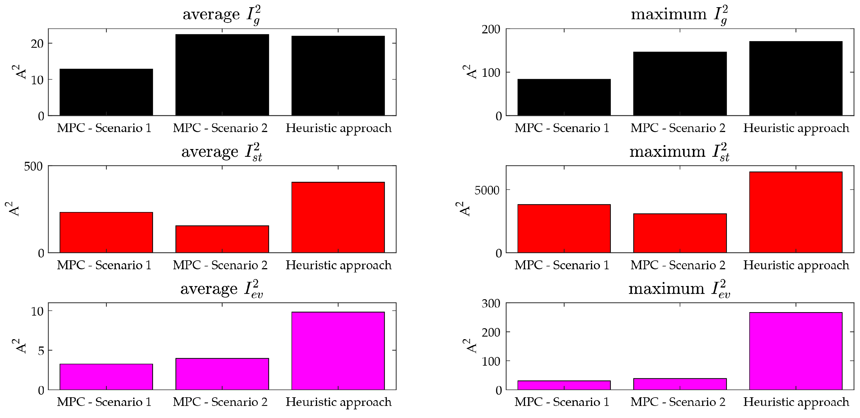
Statistical results from the different cases are shown in Figure 6; the MPC substantially exhibits the advantage of providing lower $I_g^2$ (which is related to network losses) and lower $I_{st}^2$ and $I_{ev}^2$ (which are associated with battery degradation and converter losses) with respect to the heuristic method.

6. Functional Comparison

In this section, the MPC approach and the heuristic method are compared from a functional perspective. As in the example in the previous section, a seven-day simulation period is considered. The ESS and the EVB have the same characteristics as those introduced in Section 5. The planned schedule of departures and arrivals of the EV is provided in

Table 3. Functional comparison: planned departure and arrival times and EVB energy consumption.

Day of the Week	Departures	Arrivals	Energy Consumption
Wednesday	6 a.m.	18 p.m.	10.80 kWh
Thursday	6 a.m.	18 p.m.	7.2 kWh
Friday	6 a.m.	21 p.m.	36 kWh
Saturday	7 a.m.	22 p.m.	36 kWh
Sunday	7 a.m.	20 p.m.	36 kWh
Monday	6 a.m.	18 p.m.	10.80 kWh
Tuesday	6 a.m.	18 p.m.	3.60 kWh

. Unlike in the example in the previous section, a much greater discharge of the EV battery in three days of the week (i.e., Friday, Saturday and Sunday) is considered. During the daytime, the EV is assumed to exploit all available energy stored in the battery (36 kWh).

In the tests performed here, the control sample time is set to one hour for both control approaches; the MPC is implemented with a one-day prediction horizon. As far as the grid power is concerned, $P_{g,max}$ is set to 3 kW.

In the simulations, the average daily energy absorbed by the loads is about 16.15 kWh/day, while the average daily energy generated by the PV panels is about 16.76 kWh/day.

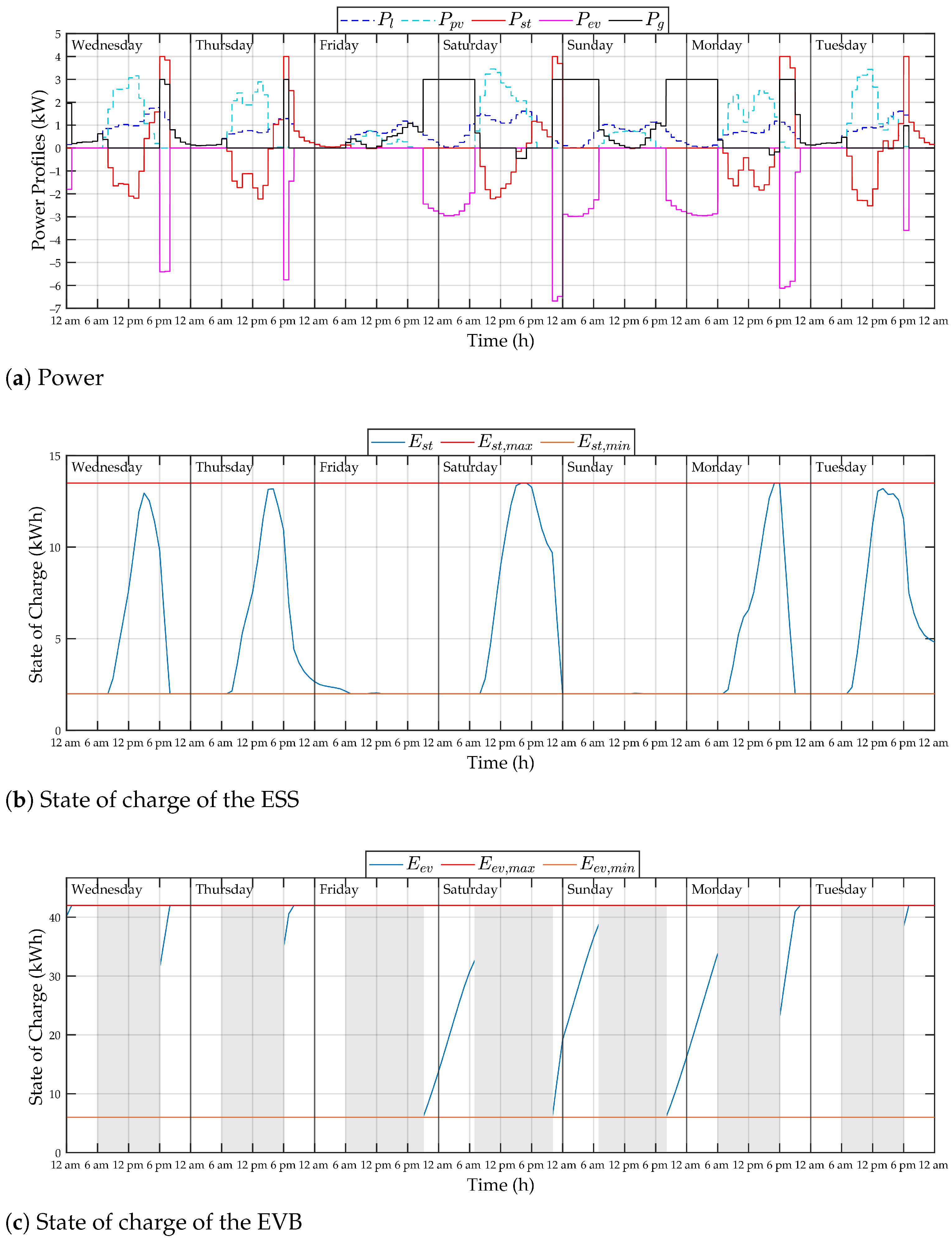
Figure 7 shows the simulation results for the MPC approach in the flat TOU rate scenario. It is worth noting that, on Friday, Saturday, and Sunday, MPC successfully manages the energy resources (i) to fully charge the EVB during the nighttime and (ii) to respect the upper bound of 3 kW for the maximum power absorbed from the grid. On the one hand, during the daytime on Friday and Sunday, since there is lack of production, the predictive controller uses the grid to charge the ESS until reaching the state of charge that ensures a full EVB at the departure time of the following day. On the other hand, on Saturday, the MPC smartly manages available resources by exploiting the grid to satisfy the demand in the afternoon with the aim of leaving enough energy for nighttime charging in the ESS.

Figure 8 shows the simulation results for the heuristic approach. It is worth noting that, unlike the MPC, the heuristic approach is not able to ensure a full EVB before the departure times on Saturday, Sunday, and Monday. In detail, at the arrival time on Friday and Sunday, the ESS is empty, so it cannot provide energy to the EVB during the next night. On Saturday, the heuristic approach badly manages the ESS, since it exploits the stored energy in the afternoon before the arrival time of the EV; the remaining energy at the arrival time is not enough to guarantee a full EVB on Sunday morning. As a consequence of poor resource management, there is a decrease in the mileage with respect to what is planned (Table 3) on Saturday and Sunday because the driver has to satisfy the lower bound constraint of the EVB (6 kWh). Indeed, differently from the MPC case, the actual EVB energy consumption obtained with the heuristic method decreases by about 26% on Saturday and 9% on Sunday. It is worth remarking that, in this scenario, an economic comparison between the MPC and the heuristic method would be meaningless, as the mileage of the EV is different in the two cases.

In the above example, the heuristic approach shows the functional disadvantage of not being able to fully charge the EVB during the nighttime; on the other hand, this is possible through the use of predictive control techniques that manage the available resources by exploiting future information. The previous example highlights the potential for MPC in future contexts, since, by smartly managing available energy resources, it can guarantee the desired functionalities, which cannot be always ensured by simple heuristic techniques. Moreover, while satisfying the additional requirements of EV charging, the MPC is shown to be capable of keeping the peak power absorption from the grid constrained within nominal limits, which is an aspect of relevant concern considering the expected widespread use of electric vehicles.

7. Conclusions

This paper shows the application of model predictive control for the efficient management of prosumers’ energy resources in the presence of local energy storage capabilities and an electric vehicle (EV). The aim of the predictive control developed here is the minimization of the economic cost with the constraint of ensuring a full EV battery at departure times. The proposed predictive approach is compared with a heuristic method that manages the available resources in an instantaneous rule-based manner. The simulation results show that, on the one hand, the MPC provides lower costs in scenarios in which both strategies are able to fully charge the EV battery during the night. On the other hand, it can guarantee a full recharge in scenarios in which the heuristic method is not capable of doing so. In summary, the simple scenario considered here allowed us to highlight the remarkable advantages of using predictive approaches in such an application, even while considering different energy pricing schemes. It is shown that the MPC algorithm, through optimal management of the available resources, allows one to (i) to meet functional objectives, such as the full recharge of the EV battery, (ii) allow the economic management of local resources, (iii) reduce rms current values at the interface with the mains and the local energy storage system, and (iv) keep the power exchanged with the mains within nominal ranges.

Future developments of the presented research may include the study of the effect of prediction errors on the performance of the MPC procedure and a sensitivity analysis of the MPC’s performance as different parameters vary (e.g., length of the prediction horizon, energy storage capacities, PV system size).