Application of the Harmonic Balance Method for Spatial Harmonic Interactions Analysis in Axial Flux PM Generators

Abstract

In this paper, an application of the Harmonic Balance Method (HBM) for analysis of Axial Flux Permanent Magnet Generator (AFPMG) is carried out. Particular attention was paid to development of mathematical model equations allowing to estimate the machine properties, without having to use quantitative solutions. The methodology used here allowed for precise determination of Fourier spectra with respect to winding currents and electromagnetic torque (both quantitatively and qualitatively) in steady state operation. Analyses of space harmonic interaction in steady states were presented for the three-phase AFPMG. Satisfactory convergence was between the results of calculations and measurements which confirmed the initial assumption that the developed circuit models of AFPMG are sufficiently accurate and can be useful in the diagnostic analyses, tests and the final stages of the design process.

1. Introduction

Interest in Permanent Magnet (PM) synchronous generators is associated with a global trend to support local energy supplied with renewable energy sources such as wind or water power, in which synchronous generators excited by permanent magnets are being increasingly applied [1,2,3,4,5,6]. Generators in this class of applications typically have a cylindrical rotor with surface-mounted magnets, but axial magnetic flux disc generator solutions are also very popular [7,8]. For this reason, both design and mathematical modelling techniques of these machines are being constantly developed and improved [9,10,11,12,13,14,15,16,17,18,19,20,21,22,23,24,25]. The Axial Flux PM (AFPM) generator deserves special attention due to their variety of designs and popularity in low-power home applications. This article is a continuation of the authors’ papers [9,10,11] on AFPMG modeling, however it does not limit the possibility of applying the presented methodology to other constructions of PM generators.

Mathematical models of PM synchronous generators should provide the possibility of solving, in a relatively simple manner, various operational issues associated with the generation of electrical energy. For this purpose, the most suitable are so-called circuit models, commonly used in conventional machines [9,10,11,12,16,22] and the purpose of this paper is to extend the mathematical modeling methodology for this specific class of machines, i.e., axial flux PM synchronous generators operating in steady state.

Specific design features of PM machines make the analysis of effects occurring in these machines relatively difficult. Mapping the actual shape of the air gap and PM and the real distribution of the stator windings leads to complex analytical models [13,14,15,17,19,20,25]. Finding solutions using FEM analysis [18,21,24] does not always enable a qualitative analysis of electromagnetic phenomena in the machine.

The Harmonic Balance Method (HBM) [26,27,28,29,30,31,32,33] gives the possibility of analyzing solutions of mathematic model equations of electrical machines in case of periodic variation of their coefficients; it is a simple extension of the symbolic method and leads to algebraization of the machine description in steady states. This approach is competitive with FEM analysis and allows to combine the electromagnetic phenomena occurring in the process of energy conversion in electrical machines. Such calculations are much simpler and faster.

In this paper, we focused on the methodology of HBM application for AFPMG modelling in which we also considered the influence of higher harmonics of the flux density distribution and the influence of space harmonics influence on the winding currents and the electromagnetic torque. The HBM is known and has a well-established place in the modeling of electrical machines, however, it was not widely used for AFPMG. Due to the specific design features of AFPM machines, the methodology of modeling with the use of HBM [26,27,28,29,30] must be adapted to them. In the presented approach, the model parameters are linear because there are no nonlinearity problems for the AFPMG structure.

The main task of this presented study is full use of the HBM in analysis of the steady-state of [30,31] AFPM generators. This approach has not been widely published for this class of machines. The issue was investigated to determine whether by means of mathematical modelling and numerical calculations it is possible to distinguish and quantify the interaction of spatial harmonics [26,29,30,31]. This paper presents developed HBM mathematical models that enable the execution of such analyses also for diagnostic purpose. Another aspect of the usefulness of mathematical models is, in addition to the analysis of these effects that are usually of parasitic nature, the possibility to synthesize harmonic interactions at the stage of designing the machine. In steady-state operation, the mathematical model of a PM machine is reduced to a system of linear differential equations with periodically varying coefficients [30,31]. A detailed analysis and solution of this system of equations using the HBM enables qualitative (frequency determination) and quantitative (amplitude determination) assessment of Fourier spectrums of currents and electromagnetic torque.

2. Harmonic Balance Method for Modeling PM Machines

2.1. General Assumptions

In permanent magnet excited machines, the most important energy processing elements are coils that form windings and permanent magnets. For co-energy to clearly describe winding states of their characteristics, relationships describing the linkage fluxes as functions of currents, and the rotor position must be unambiguous. It is a fundamental assumption, and it means that it is not possible to include the phenomenon of magnetic hysteresis. Changes in the energy state of the permanent magnet under the influence of coil currents occur in accordance with the inner hysteresis loop, called a return curve, which is very narrow for modern magnets, and is usually approximated by a straight line, as a result the hysteresis effect practically disappears. In modern permanent magnets of rare earth metals, the return curves additionally coincide with the demagnetization curve for its rectilinear section. Therefore, it can be assumed that for changes induced by winding currents, the permanent magnet operating point moves along unique demagnetization curve, which corresponds to uniqueness of changes in the co-energy of a permanent magnet [11,31]. Since iron cores of the stator and rotor have very high magnetic permeability compared to air and rare earth magnet materials, it can be assumed that the energy of the magnetic field concentrates mainly in the air gap and permanent magnets, which means that magnetic voltage drops in the machine’s iron yokes are linear and can be included in permeance function, which describes machine magnetic geometry or these drops can be neglected. Assumption of linearity of the magnetic circuit is the key element for further analyses contained in the paper. This assumption in PM machines is usually acceptable and allows for determination of winding characteristics and the relationship describing co-energy, using self and mutual inductances. Windings will then be described by functions depending on the angle of rotor position and are additionally linear functions of currents. These functions also have additional elements representing flux linkage excited by PM, which is also a function of the rotation angle $\phi$.

Using Lagrange’s formalism based on the characteristics of windings and co-energy function with respect to electromechanical components of the entire system lead to mathematical equations of 3-phase PM machines. The mathematical model equations of PM machine can be written generally in a standard matrix form [11,31]

$$\begin{array}{l}\frac{d}{dt}\{L(\phi )\cdot i+{\Psi }_{PM}(\phi )\}+R_s\cdot i=u\\ J\frac{d\omega }{dt}=T_{em}(\phi ,i_1,i_2,i_3)+T_{cog}(\phi )+T_E-D\cdot \omega \\ \frac{d\phi }{dt}=\omega \end{array}$$

(1)

wherein electromagnetic torque

$$T_{em}(i_1,i_2,i_3,\phi )=\frac{1}{2}{i}^T\cdot \frac{\partial }{\partial \phi }L(\phi )\cdot i+i^T\cdot \frac{\partial }{\partial \phi }{\Psi }_{PM}(\phi )$$

(2)

cogging torque

$$T_{\mathrm{cog}}(\phi )=\frac{\partial E_{0\mathrm{PM}}^{}(\phi )}{\partial \phi }$$

(3)

where:

$$L(\phi )=L_{\sigma s}+L_s(\phi )=\left[\begin{array}{ccc}{L}_{\sigma s}& & \\ & L_{\sigma s}& \\ & & L_{\sigma s}\end{array}\right]+\left[\begin{array}{ccc}{L}_{11}(\phi )& L_{12}(\phi )& L_{13}(\phi )\\ L_{21}(\phi )& L_{22}(\phi )& L_{23}(\phi )\\ L_{31}(\phi )& L_{32}(\phi )& L_{33}(\phi )\end{array}\right]$$

(4)

$$i=\left[\begin{array}{c}{i}_1\\ i_2\\ i_3\end{array}\right]\hspace{0.17em}\hspace{0.17em}\hspace{0.17em}\hspace{0.17em}\hspace{0.17em}\hspace{0.17em}u=\left[\begin{array}{c}{u}_1\\ u_2\\ u_3\end{array}\right]\hspace{0.17em}\hspace{0.17em}\hspace{0.17em}\hspace{0.17em}\hspace{0.17em}\hspace{0.17em}\hspace{0.17em}\hspace{0.17em}\hspace{0.17em}{\Psi }_{PM}(\phi )=\left[\begin{array}{c}{\psi }_{PM1}(\phi )\\ {\psi }_{PM2}(\phi )\\ {\psi }_{PM3}(\phi )\end{array}\right]\hspace{0.17em}\hspace{0.17em}\hspace{0.17em}\hspace{0.17em}\hspace{0.17em}\hspace{0.17em}\hspace{0.17em}\hspace{0.17em}\hspace{0.17em}\hspace{0.17em}{R}_s=\left[\begin{array}{ccc}{R}_s& & \\ & R_s& \\ & & R_s\end{array}\right],$$

(5)

$i_a \mathrm{and} u_a$—stator phase “a” current and voltage, a = 1, 2, 3; $R_s$—stator winding resistance; ${\psi }_{\mathrm{PM}\hspace{0.17em}a}(\phi )$—flux linkage of winding “a”, produced by permanent magnets, a = 1, 2, 3; $L_{\sigma s}$, $L_{aa}(\phi )$, $L_{ab}(\phi )$—represents the inductance of the windings (leakage, self and mutual) a, b = 1, 2, 3; $E_{0\mathrm{PM}}^{}(\phi )$—component of PM machine co-energy independent of winding currents; $\omega$—rotor speed; $T_E$—external driving torque; $D$—damping coefficient.

The equation of electromechanical torque (2) contains the reluctance torque component and the main electromagnetic torque generated by the interaction between winding and permanent magnet fluxes. Torque produced in a zero-current state (3), is called cogging torque $T_{\mathrm{cog}}$ and is formed by the tangential forces acting on the slot walls and edges of the permanent magnet poles. The above equations are common, and their structure is very similar to Lagrange equations concerning conventional electric machines. Additional elements appear due to the presence of PM and the inductance must consider the existence of PM in the magnetic circuit of the machine.

Mathematical models of electric machines used in spatial harmonic interactions impact assessment, require correct identification of the qualitative characteristics of flux linkage, as a function of the angle of rotor position [26,29,30,31]. The geometry of the magnetic circuit of PM machines is very diverse and simple relationships, sufficiently accurate for classic machines cannot always be used for PM machines. In many cases, the calculation of equation parameters for PM machines will require a numerical determination of the field distribution (FEM analysis) in the machine, and, on this basis, approximation of the necessary coefficients.

Generally, for most of the designed symmetrical windings, MMF harmonics belong to set $\{\dots -5p,-3p,-p,p,3p,5p\dots \}$, where “p” is number of machine pole pairs. The magnetic circuit may be characterized using unit permeance function. In this case, when we consider regular shape of the magnetic circuit the inductance matrix can be written in the following form [26,29,31]

$$L_s(\phi )={\displaystyle \sum _{n=0,\pm 2p,\pm 4p,\dots }\hspace{0.17em}\hspace{0.17em}{L}_n^{}}\cdot e^{jn\phi }$$

(6)

and the vector of PM flux linkages can be presented as

$${\Psi }_{PM}^{}(\phi )={\displaystyle \sum _{\varsigma =\pm p,\pm 3p,\pm 5p\dots }{\Psi }_{\varsigma }^{PM}\cdot e^{j\varsigma \phi }}$$

(7)

2.2. Aplication of HBM for Modeling Spatial Harmonic Interaction in 3-Phase PM Generators

The main problem here is to show how to define the parameters of the model, which should highlight the impact of all relevant harmonics of a spatial field distribution in the machine, and the conversion of the mathematical model to be able to track the interactions of these harmonics.

Very useful in determining this is the symmetrical components transform, which describes the machine in orthogonal bases, and puts in order inductance matrices and vectors of PM flux linkages, so that based on equations, we can analyze how spatial harmonics affect currents and electromagnetic torque [26,29,30,31].

If mathematical model Equation (1) is transformed into symmetrical components, using a matrix transformation

$$T_3=\frac{1}{\sqrt{3}}{\left[\begin{array}{ccc}1& 1& 1\\ 1& \underset{¯}{a}& {\underset{¯}{a}}^2\\ 1& {\underset{¯}{a}}^2& \underset{¯}{a}\end{array}\right]}_{(3x3)} \mathrm{where} \underset{¯}{a}=e^{j\frac{2\pi }{3}}$$

(8)

then, the machine voltage equations take the form

$$\frac{d}{dt}\{[L_{\sigma s}^{}+L_s^s(\phi )]\cdot i^s\}+\frac{d}{dt}{\Psi }_{PM}^s(\phi )+R_s\cdot i^s=u^s$$

(9)

and the equation for the electromagnetic torque can be defined as

$$T_{em}(i^{s0}\hspace{0.17em}\hspace{0.17em}{i}^{s1}\hspace{0.17em}\hspace{0.17em}{i}^{s2},\phi )=\frac{1}{2}{(\stackrel{\vee }{i^s})}^T\cdot \frac{\partial }{\partial \phi }{L}_s^s(\phi )\cdot i_{}^s+{(\stackrel{\vee }{i^s})}^T\cdot \frac{\partial }{\partial \phi }{\Psi }_{PM}^s(\phi )$$

(10)

where:

$$u^s=T_3\hspace{0.17em}\cdot \hspace{0.17em}u\hspace{0.17em}\hspace{0.17em}\hspace{0.17em};\hspace{0.17em}\hspace{0.17em}\hspace{0.17em}{u}^s={[u^{s0}\hspace{0.17em}\hspace{0.17em}{u}^{s1}\hspace{0.17em}\hspace{0.17em}{u}^{s2}]}^T\hspace{0.17em}; i^s=T_3\cdot \hspace{0.17em}i\hspace{0.17em}\hspace{0.17em}\hspace{0.17em}\hspace{0.17em}\hspace{0.17em}\hspace{0.17em};\hspace{0.17em}\hspace{0.17em}\hspace{0.17em}{i}^s={[i^{s0}\hspace{0.17em}\hspace{0.17em}{i}^{s1}\hspace{0.17em}\hspace{0.17em}{i}^{s2}]}^T$$

(11)

$$L_s^s(\phi )=T_3\cdot L_s(\phi )\cdot T_3{}^{-1}={\displaystyle \sum _n\hspace{0.17em}\hspace{0.17em}{L}_n^s}\cdot e^{jn\hspace{0.17em}\phi }$$

(12)

$${\Psi }_{PM}^s(\phi )=T_3\cdot {\Psi }_{PM}^{}(\phi )={\displaystyle \sum _{\varsigma }{\Psi }_{\varsigma }^{PMs}\cdot e^{j\varsigma \phi }}={[{\psi }^{s0}(\phi )\hspace{0.17em}\hspace{0.17em}\hspace{0.17em}\hspace{0.17em}{\psi }^{s1}(\phi )\hspace{0.17em}\hspace{0.17em}\hspace{0.17em}\hspace{0.17em}{\psi }^{s2}(\phi )]}^T$$

(13)

If we consider a synchronous PM machine operating in generator mode, then winding current arrows must indicate proper energy flow direction. In the considerations, receiver current arrows according to Figure 1 were adopted. For such adopted arrows, it is understood that the external torque $T_E>0$ is for generator operation and then the values of currents obtained from the solutions of the machine model equations will have a negative sign.

Circuit Equation (9) for generator mode shown in Figure 1 can be defined as

$$\frac{d}{dt}\{(L_{\sigma s}^{}+L_s^s(\phi )+L_L^s)\cdot i^s\}+(R_s+R_L^s)\cdot i^s=e_L^s-\frac{d}{dt}{\Psi }_{PM}^s(\phi )$$

(14)

where:

$$R_L^s=T_3\cdot \left[\begin{array}{ccc}{R}_{L1}& & \\ & R_{L2}& \\ & & R_{L3}\end{array}\right]\cdot \hspace{0.17em}{T}_3{}^{-1}+\left[\begin{array}{ccc}3R_N& & \\ & 0& \\ & & 0\end{array}\right]; L_L^s=T_3\hspace{0.17em}\cdot \hspace{0.17em}\left[\begin{array}{ccc}{L}_{L1}& & \\ & L_{L2}& \\ & & L_{L3}\end{array}\right]\cdot \hspace{0.17em}{T}_3{}^{-1}$$

(15)

If we assume the EMFs on load side to be a balanced three-phase voltage system, although this assumption is not mandatory, then it will correspond to the generator coupled with the grid. These voltages in symmetrical components are of the form

$$e_L^s=T_3\cdot \sqrt{2}\hspace{0.17em}{E}_{Sph}\left[\begin{array}{c}\cos ({\omega }_0\hspace{0.17em}t+{\beta }_0)\\ \cos ({\omega }_0\hspace{0.17em}t+{\beta }_0-\raisebox{1ex}{$2\pi $}\!\left/ \!\raisebox{-1ex}{$3$}\right.)\\ \cos ({\omega }_0\hspace{0.17em}t+{\beta }_0-\raisebox{1ex}{$4\pi $}\!\left/ \!\raisebox{-1ex}{$3$}\right.)\end{array}\right]={\displaystyle \sum _{\eta =\pm 1}}{E}_{\eta }^s\cdot e^{j\eta \hspace{0.17em}{\omega }_0\hspace{0.17em}t}=E_1^s\cdot e^{j\hspace{0.17em}{\omega }_0\hspace{0.17em}t}+E_{-1}^s\cdot e^{-j\hspace{0.17em}{\omega }_0\hspace{0.17em}t}=\left[\begin{array}{c}0\\ \underset{¯}{E}\\ 0\end{array}\right]\cdot e^{j\hspace{0.17em}{\omega }_0\hspace{0.17em}t}+\left[\begin{array}{c}0\\ 0\\ \stackrel{\vee }{\underset{¯}{E}}\end{array}\right]\cdot e^{-j\hspace{0.17em}{\omega }_0\hspace{0.17em}t}$$

(16)

where: $\underset{¯}{E}=E_S\cdot e^{j\hspace{0.17em}{\beta }_0\hspace{0.17em}}=\sqrt{\frac{3}{2}} E_{Sph}\cdot e^{j\hspace{0.17em}{\beta }_0}$, $E_{ph}$ is the RMS value of grid phase voltage (line-neutral).

The steady state is considered when angular velocity of the rotor is constant $\omega =\Omega$ then $\phi =\Omega \cdot t+{\phi }_0$. The angle value ${\phi }_0$ is related to the generator load. This angle will be important only in case of the generator’s cooperation with the power grid (for standard monoharmonic models $p{\phi }_0-{\beta }_0=\vartheta +\frac{3}{2}\pi$, where $\vartheta$ is a generator power angle). If synchronous steady-state dependency ${\omega }_0=p\Omega$ is fulfilled, then the inductance matrix (12) and vector of PM flux linkages (13) become periodic, and we can assume solutions for the set of Equation (14), as

$$i^s={\displaystyle \sum _{\nu }}{I}_{\nu }^s\cdot e^{j\nu \Omega t}; I_{\nu }^s={[{\underset{¯}{I}}_{\nu }^{s0}\hspace{0.33em}\hspace{0.33em}{\underset{¯}{I}}_{\nu }^{s1}\hspace{0.17em}\hspace{0.17em}\hspace{0.17em}\hspace{0.17em}{\underset{¯}{I}}_{\nu }^{s2}]}^T$$

(17)

Solutions (17) fulfill, according to the HBM [26,29,30,31], an infinite dimensional system of algebraic equations

$$\begin{gathered} \begin{array}{c}\hfill diag\left[\begin{array}{c}⋮\\ j3p\Omega E_{\left(3x3\right)}\\ jp\Omega E_{\left(3x3\right)}\\ -jp\Omega E_{\left(3x3\right)}\\ -j3p\Omega E_{\left(3x3\right)}\\ ⋮\end{array}\right]·\left[\begin{array}{cccccc}\ddots & & ⋮& ⋮& ⋮& \\ & L_0^{ss}+L_L^s& L_{2p}^{ss}& L_{4p}^{ss}& L_{6p}^{ss}& \cdots \\ \cdots & L_{-2p}^{ss}& L_0^{ss}+L_L^s& L_{2p}^{ss}& L_{4p}^{ss}& \cdots \\ \cdots & L_{-4p}^{ss}& L_{-2p}^{ss}& L_0^{ss}+L_L^s& L_{2p}^{ss}& \cdots \\ \cdots & L_{-6p}^{ss}& L_{-4p}^{ss}& L_{-2p}^{ss}& L_0^{ss}+L_L^s& \\ & ⋮& ⋮& ⋮& & \ddots \end{array}\right]·\left[\begin{array}{c}⋮\\ I_{3p}^s\\ I_p^s\\ I_{-p}^s\\ I_{-3p}^s\\ ⋮\end{array}\right]+ \\ +diag\left[\begin{array}{c}⋮\\ R_s^{}+R_L^s\\ R_s^{}+R_L^s\\ R_s^{}+R_L^s\\ R_s^{}+R_L^s\\ ⋮\end{array}\right]·\left[\begin{array}{c}⋮\\ I_{3p}^s\\ I_p^s\\ I_{-p}^s\\ I_{-3p}^s\\ ⋮\end{array}\right]=\left[\begin{array}{c}⋮\\ 0\\ E_1^s\\ E_{-1}^s\\ 0\\ ⋮\end{array}\right]-diag\left[\begin{array}{c}⋮\\ j3p\Omega E_{\left(3x3\right)}\\ jp\Omega E_{\left(3x3\right)}\\ -jp\Omega E_{\left(3x3\right)}\\ -j3p\Omega E_{\left(3x3\right)}\\ ⋮\end{array}\right]·\left[\begin{array}{c}⋮\\ {\Psi }_{3p}^{ss}\\ {\Psi }_p^{ss}\\ {\Psi }_{-p}^{ss}\\ {\Psi }_{-3p}^{ss}\\ ⋮\end{array}\right]\end{array} \end{gathered}$$

(18)

where:

$$E_{(3x3)}=\left[\begin{array}{ccc}1& & \\ & 1& \\ & & 1\end{array}\right]L_n^{ss}=\left\{\begin{array}{c}{L}_{\sigma s}^{}+L_0^s\hspace{0.17em}\hspace{0.17em}\hspace{0.17em}\hspace{0.17em}\hspace{0.17em}\hspace{0.17em}\hspace{0.17em}\hspace{0.17em}\hspace{0.17em}\hspace{0.17em}\hspace{0.17em}\hspace{0.17em}\mathrm{for}\hspace{0.17em}\hspace{0.17em}n=0\\ L_n^s\cdot e^{jn{\phi }_0}\hspace{0.17em}\hspace{0.17em}\hspace{0.17em}\hspace{0.17em}\hspace{0.17em}\hspace{0.17em}\hspace{0.17em}\hspace{0.17em}\hspace{0.17em}\hspace{0.17em}\hspace{0.17em}\hspace{0.17em}\mathrm{for}\hspace{0.17em}\hspace{0.17em}n\ne 0\end{array}\right. \mathrm{and} {\Psi }_{\varsigma }^{ss}={\Psi }_{\varsigma }^{PMs}\cdot e^{j\varsigma {\phi }_0}$$

(19)

The infinite dimensional system of linear Equation (18) with complex coefficients (19) determines the currents in the steady state. In order to make a practical use of this equation system it is necessary to limit the number of considered equations. From technical point of view, the limitations of the number equations depend on the content of the set of significant elements of PM flux linkages vector (7).

After formal mathematical transformations, similarly as it was described in [31] for analyses using HBM, we can derive the following general equation of the electromagnetic torque

$$\begin{array}{c}{T}_{em}=-\frac{1}{2}Im\{{\displaystyle \sum _{k_1=0,\pm 1,\pm 2....}^{}}\left[\begin{array}{ccccc}\cdots & \stackrel{\vee }{I_{3p}^s}& \stackrel{\vee }{I_p^s}& \stackrel{\vee }{I_{-p}^s}& \cdots \end{array}\right]\\ ·\left[\begin{array}{ccccc}& ⋮& ⋮& ⋮& \\ \cdots & 2pk{L}_{0+2pk}^{ss}& 2p(k+1)L_{2p+2pk}^{ss}& 2p(k+2)L_{4p+2pk}^{ss}& \cdots \\ \cdots & 2p(k-1)L_{-2p+2pk}^{ss}& 2pk{L}_{0+2pk}^{ss}& 2p(k+1)L_{2p+2pk}^{ss}& \cdots \\ \cdots & 2p(k-2)L_{-4p+2pk}^{ss}& 2p(k-1)L_{-2p+2pk}^{ss}& 2pk{L}_{0+2pk}^{ss}& \cdots \\ & ⋮& ⋮& ⋮& \end{array}\right]·\left[\begin{array}{c}⋮\\ I_{3p}^s\\ I_p^s\\ I_{-p}^s\\ ⋮\end{array}\right]·e^{j2pk\Omega t}\}-\\ -Im\{{\displaystyle \sum _{k=0,\pm 1,\pm 2....}^{}}\left[\begin{array}{ccccc}\cdots & \stackrel{\vee }{I_{3p}^s}& \stackrel{\vee }{I_p^s}& \stackrel{\vee }{I_{-p}^s}& \cdots \end{array}\right]·\left[\begin{array}{c}⋮\\ (2pk+3p)·{\Psi }_{2pk+3p}^{ss}\\ (2pk+p)·{\Psi }_{2pk+p}^{ss}\\ (2pk-p)·{\Psi }_{2pk-p}^{ss}\\ ⋮\end{array}\right]·e^{j2pk\Omega t}\}\end{array}$$

(20)

Equation (20) contains the reluctance torque component and the main electromagnetic torque generated by the interaction between winding currents and PM fluxes. This approach allows for the use of the developed methodology to track interactions of spatial harmonics for every topology of generators excited by permanent magnets for different levels of external asymmetry. In the case of system analysis without a neutral wire, a very large $R_N$ value should be assumed (for example 1 MΩ). Analyzing the Equations (18) and (20), it can be concluded that generally in PM machine operating in steady state, winding currents have the pulsation resulting from the interaction of spatial harmonics of orders $p\Omega , 3\hspace{0.17em}p\Omega , 5\hspace{0.17em}p\Omega , 7\hspace{0.17em}p\Omega \dots$ while electromagnetic torque contains components of the pulsation of orders $2\hspace{0.17em}p\Omega , 4\hspace{0.17em}p\Omega , 6\hspace{0.17em}p\Omega \dots$.

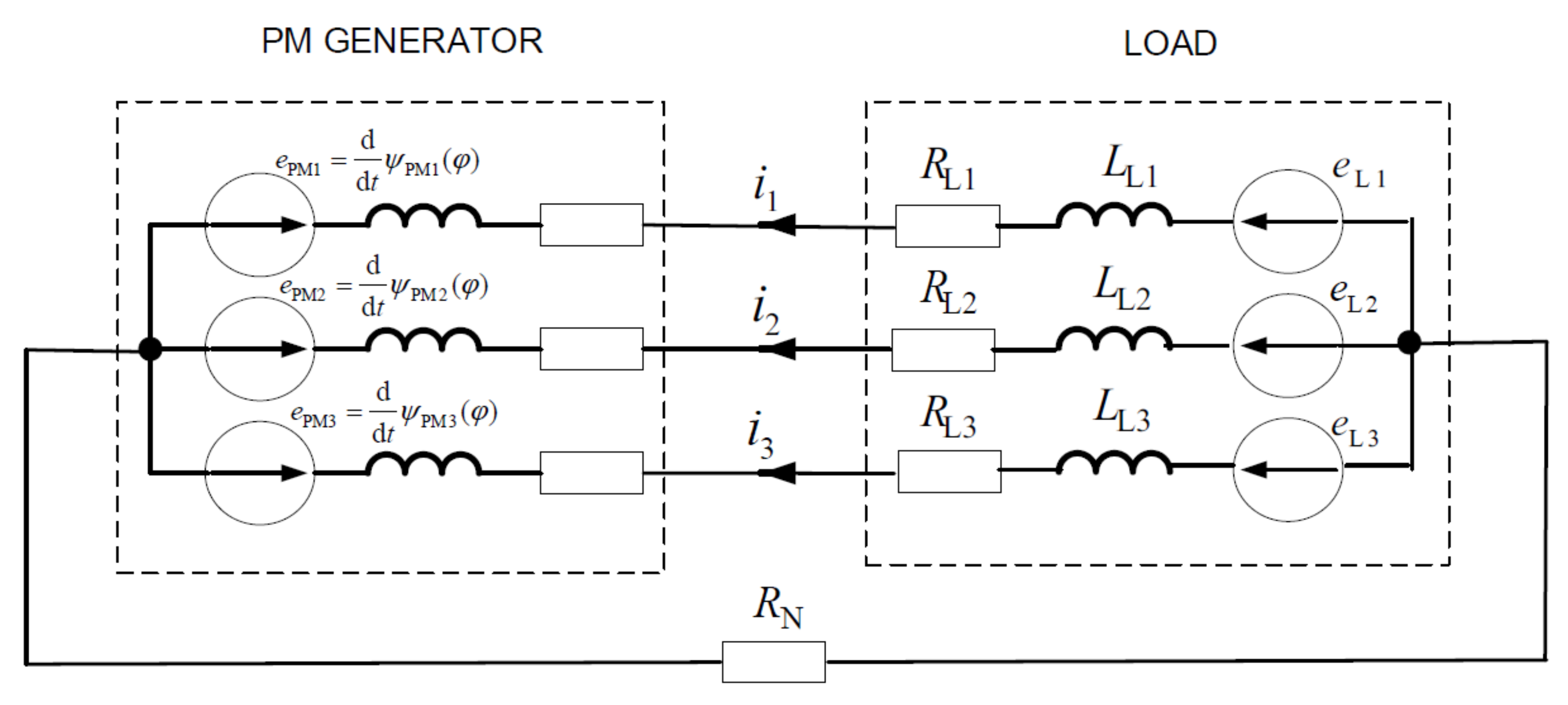
3. Model of AFPMG in Steady State Operation

3.1. Parameters of AFPMG Mathematical Model

The considerations were carried out for the three-phase AFPM generator. It can be said that this is a selected case of application of the spatial harmonic interactions modeling methodology for the PM machine presented in Section 2. The topology and structure of AFPMG are presented at Figure 2.

For AFPMG [11], due to its design features, the mathematical model is simpler and matrices of inductance $L_s(\phi )$ (6) and after transformation $L_s^s(\phi )$ (12) consist of elements independent of $\phi$

$$L_s(\phi )=L_0^{}=\left[\begin{array}{ccc}{L}_{ss}& M_{ss}& M_{ss}\\ M_{ss}& L_{ss}& M_{ss}\\ M_{ss}& M_{ss}& L_{ss}\end{array}\right]\hspace{0.17em}{L}_s^s(\phi )=L_0^s=\left[\begin{array}{ccc}{L}_0^{ss0}& 0& 0\\ 0& L_0^{ss1}& 0\\ 0& 0& L_0^{ss2}\end{array}\right]$$

(21)

where:

$$L_0^{ss0}=L_{ss}+2M_{ss} L_0^{ss1}=L_0^{ss2}=L_{ss}-M_{ss}$$

(22)

Vector of PM flux linkages ${\psi }_{PM}^{}(\phi )\hspace{0.17em}$ (7), after the symmetrical component transformation ${\psi }_{PM}^s(\phi )\hspace{0.17em}\hspace{0.17em}$ (13) contains elements which can be written as follows

$${\Psi }_{\varsigma }^{PM\hspace{0.17em}s}=\left[\begin{array}{c}{\psi }_{\varsigma }^{\hspace{0.17em}s0}\\ 0\\ 0\end{array}\right]\hspace{0.17em} \mathrm{for} \hspace{0.17em}\varsigma =\pm 3p,\pm 9p\dots \hspace{0.17em}\hspace{0.17em}\hspace{0.17em}\hspace{0.17em}\hspace{0.17em}\hspace{0.17em}\hspace{0.17em}\hspace{0.17em}\hspace{0.17em}\hspace{0.17em}\hspace{0.17em}\hspace{0.17em}\hspace{0.17em}\hspace{0.17em}\mathrm{where}\hspace{0.17em}\hspace{0.17em}\hspace{0.17em}\hspace{0.17em}{\psi }_{\varsigma }^{s0}=\sqrt{3\hspace{0.17em}}\hspace{0.17em}{\psi }_{\varsigma }^{\mathrm{PMs}}$$

(23)

$${\Psi }_{\varsigma }^{PM\hspace{0.17em}s}=\left[\begin{array}{c}0\\ {\psi }_{\varsigma }^{\hspace{0.17em}s1}\\ 0\end{array}\right]\hspace{0.17em}\hspace{0.17em} \hspace{0.17em}\mathrm{for} \hspace{0.17em}\hspace{0.17em}\hspace{0.17em}\hspace{0.17em}\varsigma =\dots -5p,p,7p\dots \hspace{0.17em}\hspace{0.17em}\hspace{0.17em}\hspace{0.17em}\mathrm{where}\hspace{0.17em}\hspace{0.17em}\hspace{0.17em}{\psi }_{\varsigma }^{s1}=\sqrt{3\hspace{0.17em}}\hspace{0.17em}{\psi }_{\varsigma }^{\mathrm{PMs}}$$

(24)

$${\Psi }_{\varsigma }^{PM\hspace{0.17em}s}=\left[\begin{array}{c}0\\ 0\\ {\psi }_{\varsigma }^{\hspace{0.17em}s2}\end{array}\right]\hspace{0.17em} \mathrm{for} \varsigma =\dots -7p,-p,5p\dots \hspace{0.17em}\hspace{0.17em}\hspace{0.17em}\hspace{0.17em}\mathrm{where}\hspace{0.17em}\hspace{0.17em}\hspace{0.17em}{\psi }_{\varsigma }^{s2}=\sqrt{3\hspace{0.17em}}\hspace{0.17em}{\psi }_{\varsigma }^{\mathrm{PMs}}$$

(25)

The method of determining the above parameters $L_{ss}$, $M_{ss}$, ${\psi }_{\varsigma }^{PM\hspace{0.17em}s}$ … for AFPMG was described in detail, for example, in the earlier papers of authors [9,10,11].

3.2. Spatial Harmonic Interaction Model for AFPMG

According to the previously presented considerations, the HBM Equations (18) and (20) for AFPM generator in the steady state can take the following form

$$\begin{gathered} \mathrm{diag}\left[\begin{array}{c}⋮\\ j3p\Omega E_{\left(3x3\right)}\\ jp\Omega E_{\left(3x3\right)}\\ -jp\Omega E_{\left(3x3\right)}\\ -j3p\Omega E_{\left(3x3\right)}\\ ⋮\end{array}\right]·\left[\begin{array}{cccccc}\ddots & & & & & \\ & L_0^{ss}+L_L^s& & & & \\ & & L_0^{ss}+L_L^s& & & \\ & & & L_0^{ss}+L_L^s& & \\ & & & & L_0^{ss}+L_L^s& \\ & & & & & \ddots \end{array}\right]·\left[\begin{array}{c}⋮\\ I_{3p}^s\\ I_p^s\\ I_{-p}^s\\ I_{-3p}^s\\ ⋮\end{array}\right]+ \\ +\mathrm{diag}\left[\begin{array}{c}⋮\\ R_s^{}+R_L^s\\ R_s^{}+R_L^s\\ R_s^{}+R_L^s\\ R_s^{}+R_L^s\\ ⋮\end{array}\right]·\left[\begin{array}{c}⋮\\ I_{3p}^s\\ I_p^s\\ I_{-p}^s\\ I_{-3p}^s\\ ⋮\end{array}\right]=\left[\begin{array}{c}⋮\\ 0\\ E_1^s\\ E_{-1}^s\\ 0\\ ⋮\end{array}\right]-\mathrm{diag}\left[\begin{array}{c}⋮\\ j3p\Omega E_{\left(3x3\right)}\\ jp\Omega E_{\left(3x3\right)}\\ -jp\Omega E_{\left(3x3\right)}\\ -j3p\Omega E_{\left(3x3\right)}\\ ⋮\end{array}\right]·\left[\begin{array}{c}⋮\\ {\Psi }_{3p}^{ss}\\ {\Psi }_p^{ss}\\ {\Psi }_{-p}^{ss}\\ {\Psi }_{-3p}^{ss}\\ ⋮\end{array}\right] \end{gathered}$$

(26)

where: $L_0^{ss}=L_{\sigma s}^{}+L_0^s\hspace{1em}\hspace{1em}{\Psi }_{\varsigma }^{ss}={\Psi }_{\varsigma }^{PMs}\cdot e^{j\varsigma {\phi }_0}$

$$T_{em}=-\mathrm{Im}\{{\displaystyle \sum _{k=0,\pm 1,\hspace{0.17em}\pm 2....}^{}\hspace{0.17em}\hspace{0.17em}\hspace{0.17em}\hspace{0.17em}\hspace{0.17em}\hspace{0.17em}\hspace{0.17em}\hspace{0.17em}\hspace{0.17em}\left[\begin{array}{ccccc}\cdots & \stackrel{\vee }{I_{3p}^s}& \stackrel{\vee }{I_p^s}& \stackrel{\vee }{I_{-p}^s}& \cdots \end{array}\right]}\cdot \left[\begin{array}{c}⋮\\ (2pk+3p\hspace{0.17em})\cdot {\Psi }_{2pk+3p}^{ss}\\ (2pk+p)\cdot {\Psi }_{2pk+p}^{ss}\\ (2pk-p)\cdot {\Psi }_{2pk-p}^{ss}\\ ⋮\end{array}\right]\cdot e^{j2p\hspace{0.17em}k\hspace{0.17em}\Omega \hspace{0.17em}\hspace{0.17em}t}\}\hspace{0.17em}$$

(27)

and matrices $R_L^s$, $L_L^s$ (15) look as follows

$$\begin{array}{c}\hfill R_L^s=\left[\begin{array}{ccc}\frac{1}{3}(R_{L1}+R_{L2}+R_{L3})+3R_N& \frac{1}{3}(R_{L1}+{\underline{a}}^2{R}_{L2}+\underline{a}{R}_{L3})& \frac{1}{3}(R_{L1}+\underline{a}{R}_{L2}+{\underline{a}}^2{R}_{L3})\\ \frac{1}{3}(R_{L1}+\underline{a}{R}_{L2}+{\underline{a}}^2{R}_{L3})& \frac{1}{3}(R_{L1}+R_{L2}+R_{L3})& \frac{1}{3}(R_{L1}+{\underline{a}}^2{R}_{L2}+\underline{a}{R}_{L3})\\ \frac{1}{3}(R_{L1}+{\underline{a}}^2{R}_{L2}+\underline{a}{R}_{L3})& \frac{1}{3}(R_{L1}+\underline{a}{R}_{L2}+{\underline{a}}^2{R}_{L3})& \frac{1}{3}(R_{L1}+R_{L2}+R_{L3})\end{array}\right]\end{array}$$

(28)

$$L_L^s=\left[\begin{array}{ccc}\frac{1}{3}(L_{L1}+L_{L2}+L_{L3})& \frac{1}{3}(L_{L1}+{\underline{a}}^2{L}_{L2}+\underline{a}{L}_{L3})& \frac{1}{3}(L_{L1}+\underline{a}{L}_{L2}+{\underline{a}}^2{L}_{L3})\\ \frac{1}{3}(L_{L1}+\underline{a}{L}_{L2}+{\underline{a}}^2{L}_{L3})& \frac{1}{3}(L_{L1}+L_{L2}+L_{L3})& \frac{1}{3}(L_{L1}+{\underline{a}}^2{L}_{L2}+\underline{a}{L}_{L3})\\ \frac{1}{3}(L_{L1}+{\underline{a}}^2{L}_{L2}+\underline{a}{L}_{L3})& \frac{1}{3}(L_{L1}+\underline{a}{L}_{L2}+{\underline{a}}^2{L}_{L3})& \frac{1}{3}(L_{L1}+L_{L2}+L_{L3})\end{array}\right]$$

(29)

Assuming a symmetrical load and introducing the following notations:

$$R_L=R_{L1}=R_{L2}=R_{L3}; L_L=L_{L1}=\hspace{0.17em}{L}_{L2}=\hspace{0.17em}{L}_{L3}; {\underset{¯}{\psi }}_{{}_{\varsigma }^{ }}^{s(0,1,2)}={\psi }_{\varsigma }^{s(0,1,2)}\cdot e^{j\varsigma {\phi }_0}=\sqrt{3\hspace{0.17em}}\hspace{0.17em}{\psi }_{\varsigma }^{PMs}\cdot e^{j\varsigma {\phi }_0}$$

(30)

it is possible to perform transformations of the system of Equation (26) rejecting the rows in which there are no voltage excitations and cutting out the corresponding columns of the system of equations. The system of Equation (26) is then significantly simplified to the following form:

$$\begin{array}{c}\mathrm{diag}\left[\begin{array}{c}⋮\\ j3p\Omega \\ jp\Omega \\ -jp\Omega \\ -j3p\Omega \\ ⋮\end{array}\right]·\left[\begin{array}{cccccc}\ddots & & ⋮& ⋮& ⋮& \\ & L^{s0}+L_L& & & & \cdots \\ \cdots & & L^{s1}+L_L& & & \cdots \\ \cdots & & & L^{s2}+L_L& & \cdots \\ \cdots & & & & L^{s0}+L_L& \\ & ⋮& ⋮& ⋮& & \ddots \end{array}\right]·\left[\begin{array}{c}⋮\\ {\underline{I}}_{3p}^{s0}\\ {\underline{I}}_p^{s1}\\ {\underline{I}}_{-p}^{s2}\\ {\underline{I}}_{-3p}^{s0}\\ ⋮\end{array}\right]+\\ +\mathrm{diag}\left[\begin{array}{c}⋮\\ R_s^{}+R_L^{}+3R_N\\ R_s^{}+R_L^{}\\ R_s^{}+R_L^{}\\ R_s^{}+R_L^{}+3R_N\\ ⋮\end{array}\right]·\left[\begin{array}{c}⋮\\ {\underline{I}}_{3p}^{s0}\\ {\underline{I}}_p^{s1}\\ {\underline{I}}_{-p}^{s2}\\ {\underline{I}}_{-3p}^{s0}\\ ⋮\end{array}\right]=\left[\begin{array}{c}⋮\\ 0\\ \underline{E}\\ \underline{\stackrel{\vee }{E}}\\ 0\\ ⋮\end{array}\right]-\mathrm{diag}\left[\begin{array}{c}⋮\\ j3p\Omega \\ jp\Omega \\ -jp\Omega \\ -j3p\Omega \\ ⋮\end{array}\right]·\left[\begin{array}{c}⋮\\ {\underline{\psi }}_{3p}^{s0}\\ {\underline{\psi }}_p^{s1}\\ {\underline{\psi }}_{-p}^{s2}\\ {\underline{\psi }}_{-3p}^{s0}\\ ⋮\end{array}\right]\end{array}$$

(31)

After the mathematical transformations of the general the electromagnetic torque Equation (27), we also obtain a simplified equation defining the electromagnetic torque for the case of a symmetrical load in the following form:

$$T_{em}=-\mathrm{Imag}\hspace{0.17em}\{\hspace{0.17em}{\displaystyle \sum _{k=0,\pm 1,\pm 2,\dots }^{}\hspace{0.17em}\left[\begin{array}{ccccc}\cdots & \stackrel{\vee }{{\underset{¯}{I}}_{3p}^{s0}}& \stackrel{\vee }{{\underset{¯}{I}}_p^{s\hspace{0.17em}1}}& \stackrel{\vee }{{\underset{¯}{I}}_{-p}^{s2}}& \cdots \end{array}\right]}\cdot \left[\begin{array}{c}⋮\\ (3p+k6p)\hspace{0.17em}{\underset{¯}{\psi }}_{3p+k6p}^{s0}\\ (p+k6p)\hspace{0.17em}{\underset{¯}{\psi }}_{p+k6p}^{s1}\\ (-p+k6p)\hspace{0.17em}{\underset{¯}{\psi }}_{-p+k6p}^{s2}\\ ⋮\end{array}\right]\cdot e^{jk6p\Omega \hspace{0.17em}t}\hspace{0.17em}\}$$

(32)

In this case, according to HBM, the vector of stator currents relates to a specific harmonic and should result in only one symmetrical non-zero component. These components can generally be related to other symmetrical components of the stator currents, but for AFPM generators there is some simplification and the components do not interact with each other. Moreover, from the symmetry properties of the system of Equation (31), it can be noticed that:

$${\underset{¯}{I}}_{\nu }^{s0}=\stackrel{\vee }{{\underset{¯}{I}}_{-\nu }^{s0}} \mathrm{and} {\underset{¯}{I}}_{\nu }^{s1}=\stackrel{\vee }{{\underset{¯}{I}}_{-\nu }^{s2}}$$

(33)

After transforming to the phase coordinates, an example of the dependency determining the time form of the current of the first phase is as follows:

$$i_1(t)=\frac{2}{\sqrt{3}}Re\{{\displaystyle \sum _{n=0}^{\infty }}\hspace{0.17em}{\underset{¯}{I}}_{(2n+1)p}^{s\hspace{0.17em}(2n+1)\hspace{0.17em}\mathrm{mod}\hspace{0.17em}3}\cdot e^{j(2n+1)\hspace{0.17em}p\hspace{0.17em}\Omega \hspace{0.17em}t}\hspace{0.17em}\}$$

(34)

During the analysis of Equation (32), it can be seen that in the case of full internal and external symmetry of the generator, components with pulsations of the order $6 p\Omega$ are present in the electromagnetic torque signal, while in the general case, according to Equation (20), additional pulsations were equal to $2 p\Omega$.

For a 3-wire system (without neutral) ${\underset{¯}{I}}_{3p+k6p}^{s0}=0 \mathrm{for} k=0, \pm 1, \pm 2, \dots$ it means that the zero-sequence current does not flow and there should be no harmonics of this order $3 p\Omega$ in the current spectrum. However, in actual measurements, it is noticed that these harmonics are present. The reason for their occurrence is not the external asymmetry of the generator, but the internal one, resulting in the generator’s EMF voltages being slightly asymmetrical. For the real construction of the generator, where asymmetries may occur, caused, e.g., by the non-uniformity of the air gap, which is often the case with disk generators, the flux linkage vectors (23)–(25) are complete and contain not only one element: ${\Psi }_{\varsigma }^{PM\hspace{0.17em}s}=\left[\begin{array}{c}{\psi }_{\varsigma }^{\hspace{0.17em}s0}\\ 0\\ 0\end{array}\right]$ but also other elements for the positive and negative components ${\Psi }_{\varsigma }^{PM\hspace{0.17em}s}=\left[\begin{array}{c}{\psi }_{\varsigma }^{\hspace{0.17em}s0}\\ {\psi }_{\varsigma }^{\hspace{0.17em}s1}\\ {\psi }_{\varsigma }^{\hspace{0.17em}s2}\end{array}\right]$ for harmonics $\varsigma =\pm 3p,\pm 9p\dots$. Then, there will also appear currents with harmonics of the order of $3\hspace{0.17em}p\Omega$, but the symmetrical components of this current will have the order of one (positive) and two (negative). Solutions in cases of internal asymmetry of the generator, as well as in case of external asymmetry, will have to be searched for using the full model according to the Equations (26) and (27).

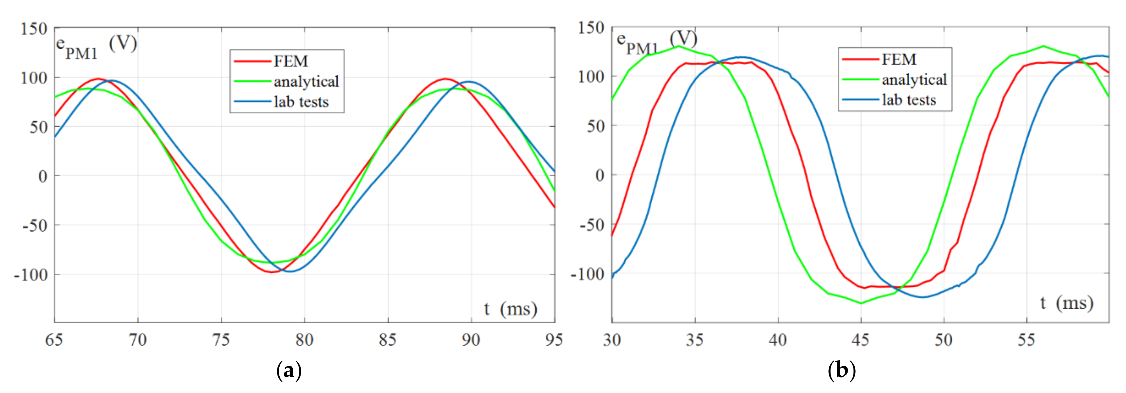
4. Laboratory Tests and Model Verifications

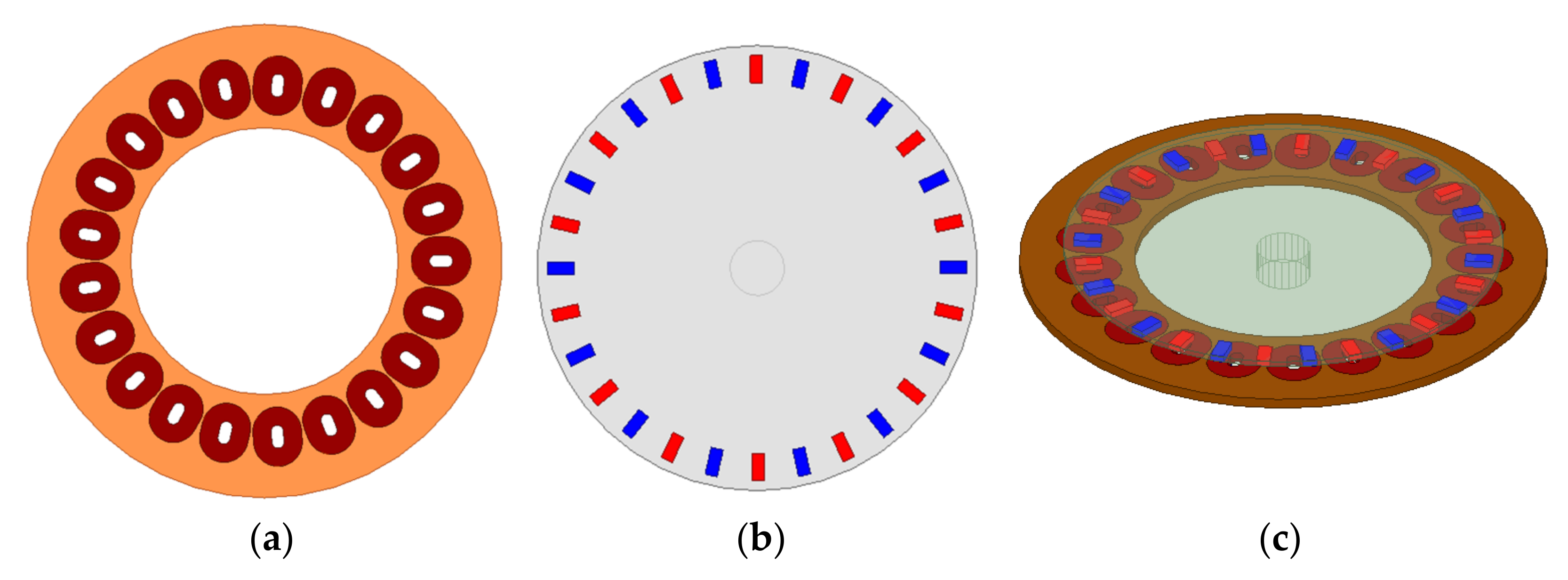
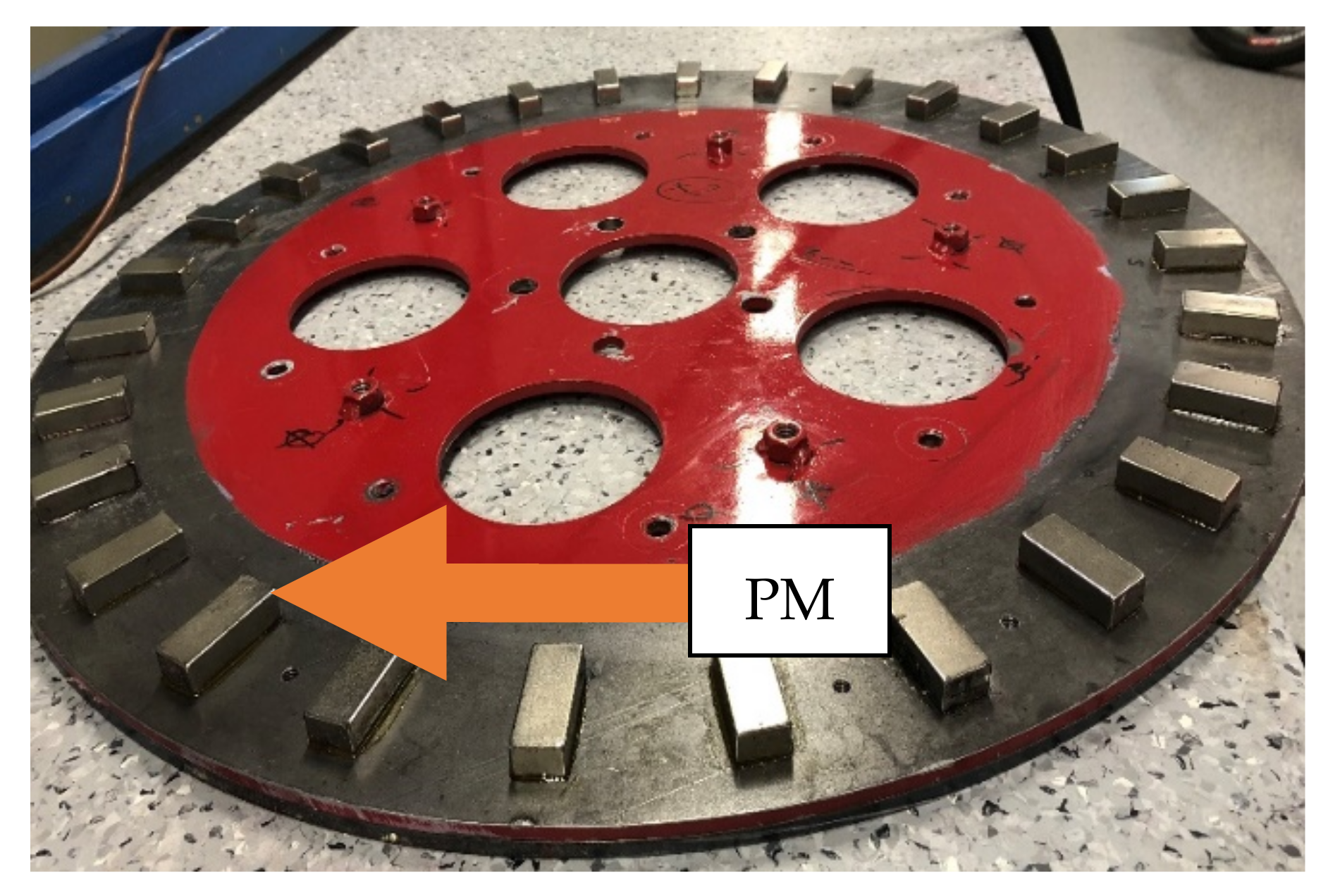
4.1. Description of Tested Generators

The verification of created models was carried out for generators with the main elements in a form of: two rotor discs (each disc with a diameter of 650 mm and 56-PM, 28-PM on one disc, $p$ = 14), a stator with a diameter of 780 mm (with 21 coils, with non-overlapping windings). The models’ verifications were extended in addition to the measurements by FEM analysis, performed in the ANSYS Maxwell environment. The generator model (Figure 3) was divided into ten regions, with a separate mesh defined for each. The total number of tetrahedral elements was 857,643.

Further analyses were carried out for two generator’s stator topologies [11]. The authors considered the following stator topologies: coreless (a) and stator with iron cores (b) placed inside the coils. The main dimensions and parameters of AFPM generators are summarized according to

Table 1. Design AFPMG data according to Figure 2.

Parameters and Dimensions of the Permanent Magnets of AFPM Generators

Magnets type: N40; Dimensions of a single magnet: 10 × 18 × 40 mm; $l_c$ = 40 mm $B_r$ = 1.2 T; $H_c$ = 899 kA/m; ${\mu }_{\mathrm{rm}}$ = 1.07; $\beta \left(r_s\right)$ = 0.0290 rad; $l_m$ = 10 mm;

Construction of the Stators in AFPM Generators

$R_i$ = 270 mm; $R_o$ = 310 mm; $r_s$ = 290 mm; $l_{\delta }$ = 26 mm; $\epsilon \left(r_s\right)$ = 0.1517 rad; $l_i$ = 15 mm—for structure with cores; $w_s$ = 980—number of turns; $R_s$ = 2 Ω

.

The laboratory equipment included a tested generator coupled with a torque measuring shaft DATAFLEX with a DC drive machine (Figure 4). All data acquisition were performed using a National Instruments measurement card. Measurements were recorded during the measurement time of 10 s with the sampling frequency of 100 kHz.

Figure 5 shows photos of the coreless (a) and with cores (b) stators. A photo of one rotor disc with the PM attached is shown in Figure 6.

4.2. Verification of Spatial Harmonic Interactions Models

The laboratory tests were carried out for modelled generators at a rotational speed of 206 rpm (48 Hz), with a three-phase (without neutral) symmetrical resistance load of the generator with the resistance value R_L = 40 Ω. The tests were performed for the AFPMG structure with a coreless stator and a stator with cores. The presented spectra (in dB) are for the adopted reference levels: 1 mV for voltages; 0.1 mA for currents and 1 mNm for torque. The parameters of the analytical models (inductances, PM flux linkage harmonics) were determined from the analytical equations presented in the authors’ base article [11]. These parameters are summarized in

Table 2. Main parameters of the analytical models.

AFPMG		Inductances		PM Flux Linkage Harmonics ${\mathit{\psi }}_{\mathit{\varsigma }}^{\mathbf{PMs}}\mathbf{=}{\mathit{\psi }}_{\mathbf{-}\mathit{\varsigma }}^{\mathbf{PMs}}$; $\mathit{\varsigma }\mathbf{=}\mathbf{p}\mathbf{,}\mathbf{3}\mathbf{p}\mathbf{,}\mathbf{5}\mathbf{p}\mathbf{,}\mathbf{7}\mathbf{p}\mathbf{,}\mathbf{9}\mathbf{p}$
		${\mathit{L}}_{\mathbf{s}\mathbf{s}}$	${\mathit{L}}_{\mathsf{\sigma }\mathbf{s}}$	${\mathit{\psi }}_{\mathbf{p}}^{\mathbf{PMs}}$	${\mathit{\psi }}_{\mathbf{3}\mathbf{p}}^{\mathbf{PMs}}$	${\mathit{\psi }}_{\mathbf{5}\mathbf{p}}^{\mathbf{PMs}}$	${\mathit{\psi }}_{\mathbf{7}\mathbf{p}}^{\mathbf{PMs}}$	${\mathit{\psi }}_{\mathbf{9}\mathbf{p}}^{\mathbf{PMs}}$
(a)	coreless stator	4.7 mH	6.2 mH	0.897 Wb	18.2 mWb	0.30 mWb	0.03 mWb	0.007 mWb
(b)	stator with cores	6.0 mH	6.2 mH	1.398 Wb	57.2 mWb	4.9 mWb	1.2 mWb	0.7 mWb

. (inductance $M_{\mathrm{ss}}\approx 0$).

First, the results for the induced EMF as a comparative measure of the PM flux linkage are presented in order to compare and indicate the main source of the generation of spatial harmonic interactions in AFPMG. The drawings below show the waveform of the induced EMF (voltage of phase one in the zero current state $e_{\mathrm{PM}1}$) for the tested generators (Figure 7) and FFT analyses (Figure 8). Results were obtained from analytical models, measurements and FEM analyses.

Table 3. Comparison of the results obtained from analytical models and laboratory tests for EMF.

AFPMG		THDEMF		EMF(RMS)
		Analytical Calculations	Measure	Analytical Calculations	Measure	|ΔEMF(%)|
(a)	coreless stator	6.1%	6.5%	61.3 V	62.6 V	2.1%
(b)	stator with cores	6.0%	7.3%	101.3 V	95.8 V	5.7%

contains comparisons of the values of the THD_EMF coefficient and the RMS values for the induced EMF of the generators, showing the relative error of calculations in relation to the measurements.

The results from the above table indicate EMF waveform distortions from the sinusoid, and thus also the winding flux linkages, although the proper verification of the presented mathematical models of spatial harmonic interaction in AFPMG required more detailed analyses of the winding currents and electromagnetic torque.

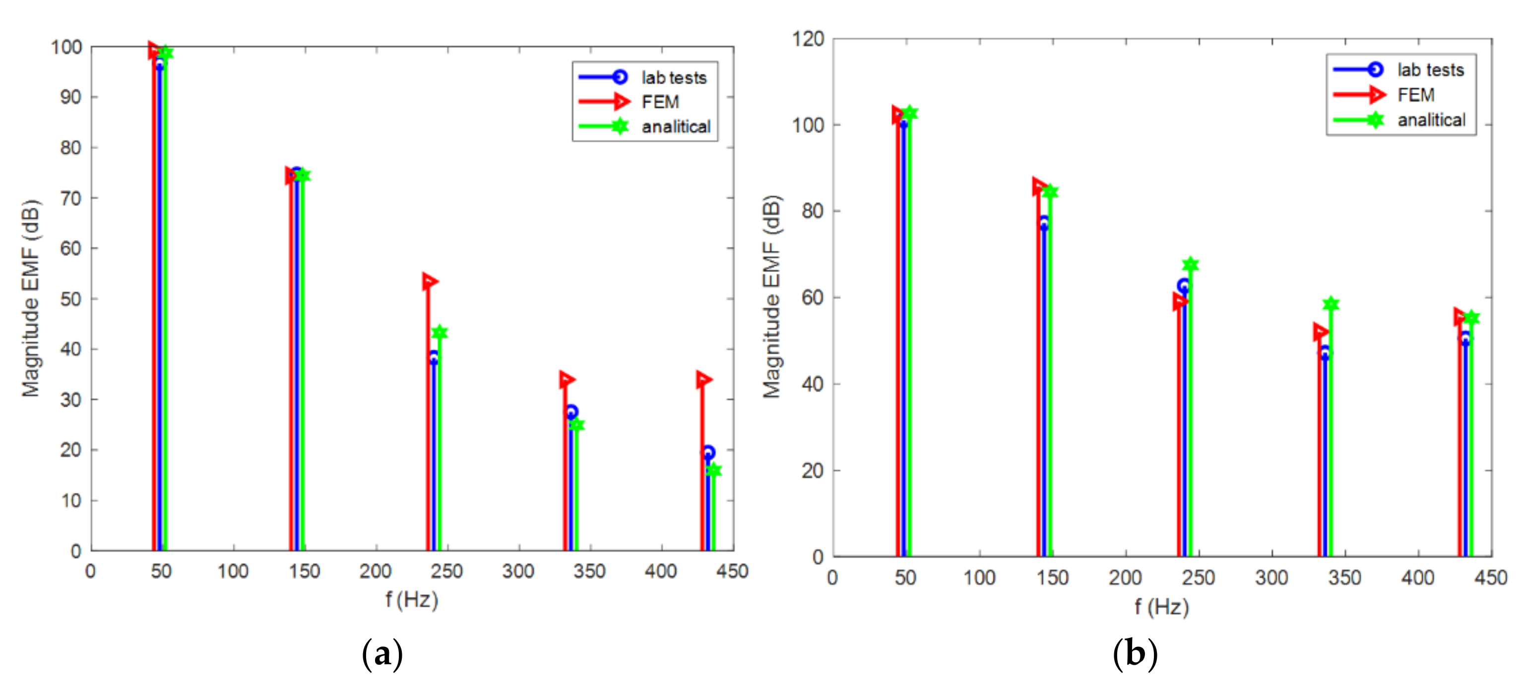
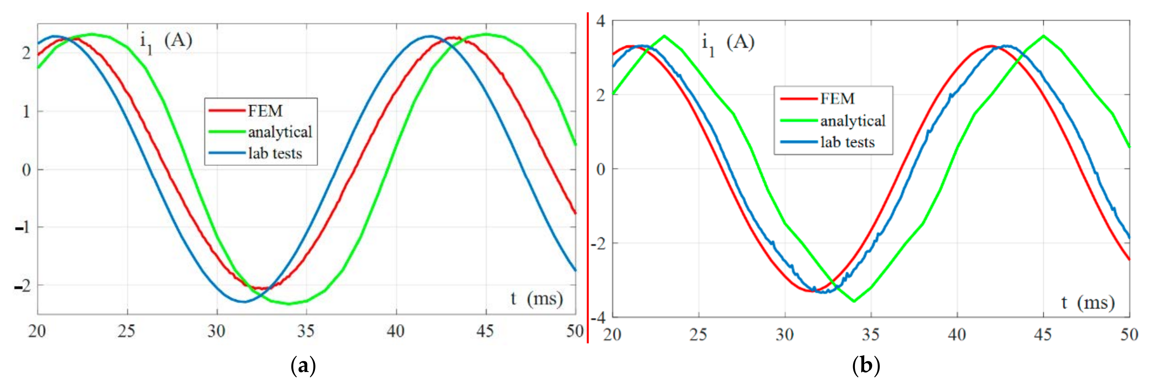
4.2.1. Verification of the Stator Currents

The drawings below (Figure 9) show the waveforms of the currents for the tested generators. The current waveforms can be considered to be similar, however, to assess them more precisely and analyse the effects of spatial harmonics interactions, FFT analyses were performed (Figure 10).

When we analyse the spectrums from Figure 10, an ideal qualitative convergence can be noticed, while quantitatively, the measurement results and the analytical calculations differ by no more than 5 dB from each other. The values of the THD_I coefficient as an indicator of the content of higher harmonics, the RMS value of currents, including the relative error of calculations with respect to the measurements (∆I_(%)), are summarized in

Table 4. Comparison of the results obtained from analytical models and laboratory tests for current $i_1$.

AFPMG		THDI		I(RMS)
		Analytical Calculations	Measure	Analytical Calculations	Measure	|∆I(%)|
(a)	coreless stator	0.16%	0.23%	1.65 A	1.69 A	2.4%
(b)	stator with cores	1.67%	1.95%	2.29 A	2.23 A	2.6%

. The obtained convergences can be considered to be satisfactory.

.

4.2.2. Verification of the Electromagnetic Torque

The verification of the results obtained for the electromagnetic torque was not fully possible due to the relatively low level of harmonics generated in the waveforms of the electromagnetic torque. The values of the analytically obtained electromagnetic torque components of the order $6 p\Omega$, $12 p\Omega$ were practically at the noise level, and it was impossible to measure them. Therefore, analysis was limited to verifying the average value of the electromagnetic torque based on analytical calculations and measurements (

Table 5. Comparison of the results obtained from analytical models and laboratory tests for average value of the electromagnetic torque.

AFPMG		Tem(AV)
		Analytical Calculations	Measure	|Tem(%)|
(a)	coreless stator	11.9 Nm	12.3 Nm	3.3%
(b)	stator with cores	31.1 Nm	29.3 Nm	6.1%

) as well as comparisons of idealized cases based on numerical FEM analyses and analytical calculations (Figure 11).

Electromagnetic torque mean value convergence up to 6%, as presented in Table 5 can be considered acceptable. The electromagnetic torque spectra presented in Figure 11 show the perfect qualitative consistency as well as the satisfactory quantitative convergence. The differences between the individual bands of the spectrum do not exceed the value of 5 dB.

5. Conclusions

The methodology presented in the article, concerning modelling of spatial harmonic interactions in AFPMG, has been confirmed for three-phase generators with a symmetrical structure which, nonetheless, do not limit the possibility of creating models using the presented methodology for the cases of machines with internal asymmetry of windings and electromagnetic circuit.

The parameters of the created models have integral form, so the accuracy of the results obtained from the presented AFPMG circuit models are limited. Certain discrepancies are present because many phenomena occurring in real models are not and cannot be represented in the mathematical models. The main reason for some discrepancies in the results are also the inaccuracy and imprecision in the assembly of the real AFPMG models.

It should be noted that for cases where there were differences in the results of calculations obtained from analytical models compared to the measurements, the results were not consistent with the use of FEM analysis either. In the presented results, in most cases (for the following quantities: EMF, currents, electromagnetic torque) the obtained results were consistent with the measurement results at a level below 10%, which can be considered as satisfactory. These results confirm the preliminary assumption that the use of HBM for AFPMG circuit models allows for sufficiently accurate analyses and the presented models can be useful for the analysis of various operational and design issues.

References

1. Chalmers, B.; Spooner, E. An axial-flux permanent-magnet generator for a gearless wind energy system. IEEE Trans. Energy Convers. 1999, 1z4, 251–257. [Google Scholar] [CrossRef]
2. Caricchi, F.; Crescimbini, F. Modular Axial-Flux Permanent-Magnet Motor for Ship Propulsion Drives. IEEE Trans. Energy Convers. 1999, 14, 673–679. [Google Scholar] [CrossRef]
3. Chen, Y.; Pillay, P.; Khan, A. PM Wind Generator Topologies. IEEE Trans. Ind. Appl. 2005, 41, 1619–1626. [Google Scholar] [CrossRef] [Green Version]
4. Chan, T.F.; Lai, L.L. An Axial-Flux Permanent-Magnet Synchronous Generator for a Direct-Coupled Wind-Turbine System. IEEE Trans. Energy Convers. 2007, 22, 86–94. [Google Scholar] [CrossRef]
5. Park, Y.-S.; Jang, S.-M.; Choi, J.-H.; Choi, J.-Y.; You, D.-J. Characteristic Analysis on Axial Flux Permanent Magnet Synchronous Generator Considering Wind Turbine Characteristics According to Wind Speed for Small-Scale Power Application. IEEE Trans. Magn. 2012, 48, 2937–2940. [Google Scholar] [CrossRef]
6. Kirtley, J.L. Permanent Magnets in Electric Machines. Electric Power Principle; John Wiley & Sons Ltd.: Hoboken, NJ, USA, 2019. [Google Scholar]
7. Gieras, J.; Wang, R.; Kamper, M. Axial Flux Permanent Magnet Brushless Machines; Springer: Berlin/Heidelberg, Germany, 2004. [Google Scholar]
8. Aydin, M.; Huang, S.; Lipo, T.A. Axial Flux Permanent Magnet Disc Machines: A Review; Wisconsin Electric Machines & Power Electronics Consortium: Madison, WI, USA, 2004. [Google Scholar]
9. Radwan-Pragłowska, N.; Borkowski, D.; Węgiel, T. Model of Coreless Axial Flux Permanent Magnet Generator. In Proceedings of the 2017 International Symposium on Electrical Machines (SME), Naleczow, Poland, 18–21 June 2017. [Google Scholar] [CrossRef]
10. Radwan-Pragłowska, N.; Węgiel, T.; Borkowski, D. Parameters identification of coreless axial flux permanent magnet generator. Arch. Electr. Eng. 2020, 67, 391–402. [Google Scholar]
11. Radwan-Pragłowska, N.; Węgiel, T.; Borkowski, D. Modeling of Axial Flux Permanent Magnet Generators. Energies 2020, 13, 5741. [Google Scholar] [CrossRef]
12. Kamper, M.J.; Wang, R.-J.; Rossouw, F.G. Analysis and performance of axial flux permanent-magnet machine with air-cored nonoverlapping concentrated stator windings. IEEE Trans. Ind. Appl. 2008, 44, 1495–1504. [Google Scholar] [CrossRef]
13. Zhilichev, Y.N. Three-dimensional analytic model of permanent magnet axial flux machine. IEEE Trans. Magn. 1998, 34, 3897–3901. [Google Scholar] [CrossRef]
14. Parviainen, A.; Niemelä, M.; Pyrhönen, J. Modeling of axial flux permanent-magnet machines. IEEE Trans. Ind. Appl. 2004, 40, 1333–1340. [Google Scholar] [CrossRef]
15. Azzouzi, J.; Barakat, G.; Dayko, B. Quasi-3D analytical modeling of the magnetic field of an axial flux permanent-magnet synchronous machine. IEEE Trans. Energy Conv. 2005, 20, 746–752. [Google Scholar] [CrossRef]
16. Wang, R.J.; Kamper, M.J.; Van der Westhuizen, K.; Gieras, J.F. Optimal design of a coreless stator axial flux permanent-magnet generator. IEEE Trans. Magn. 2005, 41, 55–64. [Google Scholar] [CrossRef]
17. Virtic, P.; Pisek, P.; Marcic, T.; Hadziselimovic, M.; Bojan, S. Analytical Analysis of Magnetic Field and Back Electromotive Force Calculation of an Axial-Flux Permanent Magnet Synchronous Generator with Coreless Stator. IEEE Trans. Magn. 2008, 44, 4333–4336. [Google Scholar] [CrossRef]
18. Hosseini, S.M.; Agha-Mirsalim, M.; Mirzaei, M. Design, prototyping, and analysis of a low cost axial-flux coreless permanent-magnet generator. IEEE Trans. Magn. 2008, 44, 75–80. [Google Scholar] [CrossRef]
19. Choi, J.-Y.; Lee, S.-H.; Ko, K.-J.; Jang, S.-M. Improved Analytical Model for Electromagnetic Analysis of Axial Flux Machines with Double-Sided Permanent Magnet Rotor and Coreless Stator Windings. IEEE Trans. Magn. 2011, 47, 2760–2763. [Google Scholar] [CrossRef]
20. Sung, S.-Y.; Jeong, J.-H.; Park, Y.-S.; Choi, J.-Y.; Jang, S.-M. Improved Analytical Modeling of Axial Flux Machine with a Double-Sided Permanent Magnet Rotor and Slotless Stator Based on an Analytical Method. IEEE Trans. Magn. 2012, 48, 2945–2948. [Google Scholar] [CrossRef]
21. Stamenkovic, I.; Milivojevic, N.; Schofield, N.; Krishnamurthy, M.; Emadi, A. Design, Analysis, and Optimization of Ironless Stator Permanent Magnet Machines. IEEE Trans. Power Electron. 2013, 28, 2527–2538. [Google Scholar] [CrossRef]
22. Jin, P.; Yuan, Y.; Minyi, J.; Shuhua, F.; Heyun, L.; Yang, H.; Ho, S.L. 3-D Analytical Magnetic Field Analysis of Axial Flux Permanent-Magnet Machine. IEEE Trans. Magn. 2014, 50, 11. [Google Scholar] [CrossRef]
23. Huang, Y.K.; Zhou, T.; Dong, J.N.; Lin, H.Y.; Yang, H.; Cheng, M. Magnetic equivalent circuit modeling of yokeless axial flux permanent magnet machine with segmented armature. IEEE Trans. Magn. 2014, 50, 1–4. [Google Scholar] [CrossRef]
24. Maryam, S.; Naghi, R.; Vahid, B.; Juha, P.; Majid, R. Comparison of Performance Characteristics of Axial-Flux Permanent-Magnet Synchronous Machine with Different Magnet Shapes. IEEE Trans. Magn. 2015, 51, 1–6. [Google Scholar]
25. Węgiel, T. Cogging torque analysis based on energy approach in surface-mounted PM machines. In Proceedings of the 2017 International Symposium on Electrical Machines (SME), Naleczow, Poland, 18–21 June 2017. [Google Scholar] [CrossRef]
26. Sobczyk, T. A reinterpretation of the Floquet solution of the ordinary differential equation system with periodic coefficients as a problem of infinite matrix. Compel 1986, 5, 1–22. [Google Scholar] [CrossRef]
27. Gilmore, R.J.; Steer, M.B. Nonlinear Circuit Analysis Using the Method of Harmonic Balance—A Review of the Art. Part, I. Introductory Concepts. Int. J. Microw. Millim.-Wave Comput.-Aided Eng. 1991, 1, 22–37. [Google Scholar] [CrossRef]
28. Gilmore, R.J.; Steer, M.B. Nonlinear Circuit Analysis Using the Method of Harmonic Balance—A Review of the Art. Part II. Advanced Concepts. Int. J. Microw. Millim.-Wave Comput.-Aided Eng. 1991, 1, 159–180. [Google Scholar] [CrossRef]
29. Sobczyk, T. Direct determination of two-periodic solution for nonlinear dynamic systems. Compel 1994, 13, 509–529. [Google Scholar] [CrossRef]
30. Rusek, J. Category, slot harmonics and the torque of induction machines. Compel 2003, 22, 388–409. [Google Scholar] [CrossRef]
31. Wegiel, T. Space Harmonic Interactions in Permanent Magnet Generator; Cracow University of Technology: Cracow, Poland, 2013. [Google Scholar]
32. Esparza, M.; Segundo-Ramirez, J.; Kwon, J.B.; Wang, X.; Blaabjerg, F. Modeling of VSC-based power systems in the extended harmonic domain. IEEE Trans. Power Electron. 2017, 32, 5907–5916. [Google Scholar] [CrossRef]
33. Ludowicz, W.; Wojciechowski, R.M. Analysis of the Distributions of Displacement and Eddy Currents in the Ferrite Core of an Electromagnetic Transducer Using the 2D Approach of the Edge Element Method and the Harmonic Balance Method. Energies 2021, 14, 3980. [Google Scholar] [CrossRef]
Figure 1. The PM generator under example load.
Energies 14 05570 g001
Figure 2. Construction of an AFPMG: (a) cross section, (b) stator, (c) rotor.
Energies 14 05570 g002
Figure 3. AFPM generator model with the ANSYS Maxwell program: (a) stator disc; (b) a rotor disc with PM arrangement; (c) assembling.
Energies 14 05570 g003
Figure 4. Laboratory test bench.
Energies 14 05570 g004
Figure 5. Stator discs; (a) coreless; (b) with cores.
Energies 14 05570 g005
Figure 6. Rotor disc.
Energies 14 05570 g006
Figure 7. Waveform of EMF (phase 1): (a) AFPMG—coreless stator; (b) AFPMG—core stator.
Energies 14 05570 g007
Figure 8. FFT spectrum of EMF (a) AFPMG—coreless stator (b) for AFPMG—core stator.
Energies 14 05570 g008
Figure 9. Waveform of current (phase 1): (a) AFPMG—coreless stator; (b) AFPMG—core stator.
Energies 14 05570 g009
Figure 10. FFT spectrum of stator current (a) AFPMG—coreless stator (b) AFPMG—core stator.
Energies 14 05570 g010
Figure 11. FFT spectrum of electromagnetic torque (a) AFPMG—coreless stator (b) AFPMG—core stator.
Energies 14 05570 g011