Abstract
Real-time transient stability studies are based on voltage angle measures obtained with phasor measurement units (PMUs). A more precise calculation to address transient stability is obtained when using the rotor angles. However, these values are commonly estimated, which leads to possible errors. In this work, the kinetic energy changes in electric machines are used as a criterion for evaluating and correcting transient stability, and to determine the precise time of insertion of a special protection system (SPS). Data from the PMU of the wide-area measurement system (WAMS) are used to construct the SPS. Furthermore, it is assumed that a microcontroller can be located in each generation unit to obtain the synchronized angular velocity. Based on these measurements, the kinetic energy of the system and the respective control action are performed at the appropriate time. The results show that the proposed SPS effectively corrects the oscillations fast enough during the transient stability event. In addition, the proposed method has the advantage that it does not depend on commonly proposed methods, such as system models, the identification of coherent machine groups, or the structure of the network. Moreover, the synchronized angular velocity signal is used, which is not commonly measured in power systems. Validation of the method is carried out in the New England power system, and the findings show that the method is helpful for real-time operation on large power systems.
1. Introduction
Transient stability is one of the least probable but most severe events faced by power systems. After the system is subjected to a large disturbance, such as a fault, one or more generators may lose synchronism with the rest of the machines if control actions are not performed. A large disturbance can cause a partial or total collapse of the network due to cascading events related to tripping the electrical machines [1]. In response to such a contingency, operators must consider applying preventive and emergency control actions to maintain stability in the power system [2]. Preventive control actions predict and evaluate the stability status and severity of a fault in real-time operation and under a certain limit, to determine if corrective action must be taken as a response. Meanwhile, emergency control initiates corrective action in real-time operations because the contingency exceeds thresholds [3].
Some conventional methods are used to study transient stability, such as numerical [4] and direct [5] techniques. Step-by-step methods (numerical integration methods) are used to solve the differential equations that represent the dynamic behavior of the power system but are time-consuming due to the computational load [4], making them unsuitable for real-time applications. In contrast, direct methods quickly determine the transient stability based on the power system energy balance [6]. Among the classic direct methods, the conventional and modified equal area criteria simplify the network by considering a generator versus an infinite bus or two machines (stable machines and unstable machines) [7,8]. However, given the growth and complexity of the power systems, this method may be too simple for multi-machine systems because the critical clearance angle depends on the critical clearance time, which is unknown [9].
Other methods reported in the literature do not require data obtained with time-domain simulations (energy functions [1,10], Lyapunov’s method [11,12], and trajectory-based methods [13,14]). For instance, in [10], the authors proposed a transient stability control system to prevent a wide-area power system blackout, in which the stability calculations were performed with data measured in the network. In [12], the authors presented an algorithm to monitor rotor angle stability that used data measured with phasor measurement units (PMUs) and helped to identify groups of coherent generators. In [13], the authors performed a real-time estimation of a stability margin under disturbances, in which data was measured from the system, and with a ball-on-concave-surface mechanics system the real-time stability status and the stability region about a monitored variable were calculated. In addition, the authors of [14] presented a prediction and control method based on trajectory information that only required the generator speed, power angle, and unbalanced power to provide the stability status of the power system. However, for multi-machine systems, these methods must identify groups of coherent generators before performing an online evaluation of the system, which is a complex and time-consuming task when considering the contingencies.
Other authors have proposed some new methods to assess transient stability under different operating conditions, requiring specialized data and representing high implementation costs. In [15], the authors proposed a method to identify transient stability boundaries based on the parametric space to identify the critical operating states; this method required the rotor-angle difference, transient kinetic energy, and transient potential energy. In [16], the authors presented an application to detect real-time transient instability by considering the characteristics of the unstable equilibrium point, the kinetic energy function, and the potential energy boundary surface; they also considered the connection of doubly fed induction generators and defined a new index for transient stability detection that required post-fault data. In [17], the authors presented the application of battery energy storage systems to relieve the generation limitation; however, this solution required a suitable location for the battery energy storage systems to absorb the kinetic energy from critical generators, and represented more costs compared to the generation tripping methods.
Some researchers have also studied transient stability based on artificial intelligent methods. For instance, in [18], the authors proposed a decision tree-based method to identify between a stable and out-of-step condition, in which the method permitted event classification; however, the method required some parameters, such as the rated power, acceleration, rotor angle, speed, and the apparent resistance measured by the relay and its rate of change. In [19], the authors proposed a generalized regression neural network based classification to predict the stability conditions of the power system; however, the method also required data generated with time-domain simulations, such as a voltage magnitude for all buses, and real and reactive powers on transmission lines. In [20], the authors presented a neural network predictive controller for the UPFC to improve the transient stability, which required training with data previously simulated and considering some restrictions. In [21], the authors used a support vector machine (SVM) classifier to predict the transient stability status of the power system, which required measured post-fault values of the generator voltages, speeds, or rotor angles. In [22], the authors presented the application of multilayer perceptron training and a support vector machine for transient stability analysis, in which a training set was required considering a large number of input variables. In [23], the authors proposed a method to evaluate the transient stability that required identifying some characteristics of the transient stability with voltage and current phasors, deviations from the center-of-inertia angle and speed, and potential- and kinetic-energy; then, these characteristic were evaluated using PMUs and used to train classification and regression trees and multivariate adaptive regression splines models. Although some of these methods are promising, data training is required and when data sampling is incomplete then simulations cannot provide a good solution for the offline, online, and real-time operations [8].
This paper uses the concept of the attached power system, which represents all the generators as a unit of a rolling ball mass on a concave surface. The criterion used in the research is related to the kinetic energy change (RACKE) [24] defined in the virtual system, which can be calculated from the generator data obtained using the wide-area measurement system (WAMS). Furthermore, the New England IEEE 39-bus was used to simulate and validate the effectiveness and accuracy of the proposed method.
The main contribution of this work is to provide a widely applicable criterion that uses a system variable, such as the angular velocity of the generators, to reduce the limitations on the structure of the network, models, system parameters, and computational load. Furthermore, a special protection system (SPS) was set up to control the transient stability. Moreover, it is possible to know the exact and opportune time to perform some control actions with the synchronized data. According to the reviewed literature, the novelty of this paper lies in the following aspects which address transient stability:
- (1).
- The synchronized angular velocity is calculated with the digital signal generated by the photoelectric effect of a transistor, which is not found in the reviewed literature;
- (2).
- The angular velocity is measured using a method that is decoupled from the synchronous machine rotor, which has not been used in previous papers;
- (3).
- The complete network is used to perform calculations and no system reductions are required, while [7] used a system reduction to find coherent groups of generators;
- (4).
- Compared to previous research, in which some authors used voltage angles to analyze transient stability [13,14], this paper proposes the use of synchronized angular velocity measured in the rotor of the machines.
Some advantages of using this method are that transient stability can be assessed directly with the synchronized angular velocity measured in the generator and it does not depend on system models, the identification of coherent machine groups, or the structure of the network. Moreover, the SPS effectively corrects the oscillations fast enough during the transient stability event. In addition, the experimental measurement was performed using an optical sensor, whose response time was 7 μs, and low-level programming which allowed greater control over the execution time of the algorithm and reduced the calculation error. Although the measurement was experimentally obtained in a single machine system, the proposed method could be scalable to large multi-machine systems.
The rest of this paper is organized as follows. Section 2 describes the mathematical model of the proposed kinetic energy change and the strategy of the SPS. In addition, the hardware used to obtain synchronized angular velocity measurements is described. Next, Section 3 presents the case study, the results, and the analysis. Finally, the conclusion of this research is presented.
2. Materials and Methods
This section presents the mathematical model of the problem and the proposed method and the hardware used to measure the angular velocity.
2.1. Mathematical Model
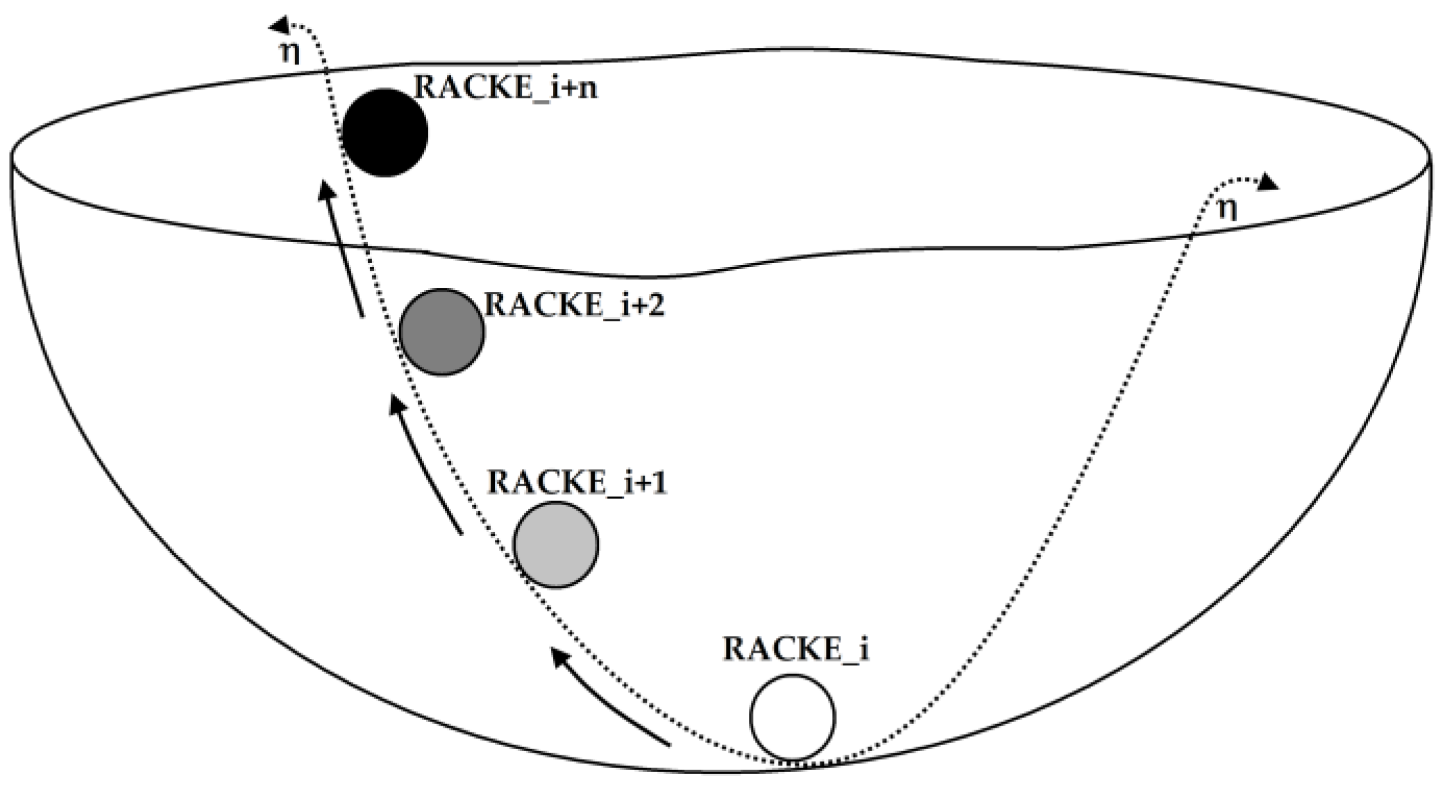
This work uses the method proposed in [9], related to the kinetic energy change index called RACKE (Rate of Change of Kinetic Energy). Thus, a criterion is proposed for transient stability control in multi-machine power systems under the concept of an attached power system, without a system reduction, similar to [25]. The original system is represented by a virtual system that considers all generators as a rolling ball mass within a surface with a limit representing the stability area (edges of the container). The instability region exists outside this limit. In this method, a simulation is carried out to, first, identify the fault clearing time, and then a transient energy margin is computed using the concept of a rotating mass system. The edge of the surface has small variations in height, as shown in Figure 1, which could represent the stress of the system during its daily operation. The criterion uses the RACKE index for the system of the rolling ball, which is calculated from the synchronized angular velocities of each of the machines of the system obtained by the measurement method proposed here.
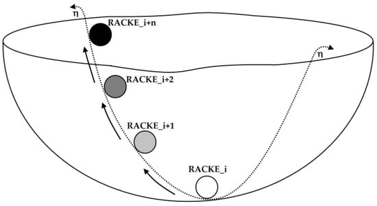
Figure 1.
Rolling ball inside a container, based on [26].
2.2. Change of Kinetic Energy
The proposed criterion does not impose limitations in the model and structure of the network, which allows for a quick evaluation of stability and the application of control actions from a single variable—in this case, the angular velocity under a disturbance. In addition, kinetic energy is an essential factor affecting the synchronism of interconnected generators in a power system. Furthermore, synchronism depends on whether or not the kinetic energy can be converted into different forms of potential energy and absorbed by the post-fault power network [6]. In other words, if the kinetic energy that is not absorbed by the system is not greater than that of the established threshold (limit), then during the post-transient event, the system will lose synchronism.
According to the laws of rotation applied to the motion of a synchronous machine, the torque is equal to the product of angular acceleration and the moment of inertia, in which net torque is the algebraic sum of all the torques acting on the machine, including shaft torque and electromagnetic torque. Thus, mathematical arrangements, beside the combination of the inertia of the generator and the prime mover, show that acceleration is created by the imbalance between the mechanical input power () and the electrical output power () of a synchronous machine, which causes an acceleration or deceleration that can be expressed as the oscillation equation presented in Equation (1). A more intuitive and detailed explanation in the development of (1) can be found in [27]:
Equation (1) assumes that (i) losses are neglected, (ii) damping torques are omitted, and (iii) mechanical power is considered as constant for transient studies [27]. On the other hand, the steady-state kinetic energy of a rotating body (turbines) is represented by Equation (2):
where is the moment of inertia and is the synchronous angular velocity (rad/s). The kinetic energy can be normalized using the inertial constant [27] as in Equation (3):
Then, the rate of change in the kinetic energy is given by Equation (4) [9]:
By substituting Equation (3) into Equation (4), the expression is obtained depending on the inertial constant as shown in Equation (5), in which is the instantaneous angular velocity of the -th generator.
Finally, an approximate notation is introduced in Equation (6) [28,29] due to the difficulty of obtaining the variable of each machine, which changes in a plant depending on the number of machines in operation:
In this study, the term is the scheduled mechanical power of each generator, which may be equal to in the normal operation or before contingencies and can be obtained by the WAMS (PMU). As previously mentioned, the mechanical power during the transient event is considered as constant, and the error can be considered as negligible. Therefore, the solution of the kinetic energy change is dependent only on the speed of the synchronous machine being able to be computed in this way for multi-machine systems with a low computational load through the synchronization of this measurement using a constellation of existing satellites (GPS, GALILEO, GLONASS, BEIDOU, and Iridium), with the signal pulse per second (PPS).
For the development of the RACKE, instead of using the inertia constant H value that is not always easy to obtain or always available, the per-unit values of the mechanical power are used, as they can be obtained from PMUs, they are easy to use, and easy to interpret. Likewise, it must be considered that in the calculation of the attached system for the development of Equation (6), it is appropriate that all machines have a similar power rate to those in the studied power system. Thus, small machines will not have such a harmful effect that leads the system to a loss of synchronism.
2.3. Rotating Mass System
The explanation of the virtualized system to a rotating mass is illustrated in Figure 1. Thus, the ball represents the steady-state stability of the power system at an equilibrium point located at the bottom of a container. When kinetic energy is injected into system, the ball will move and begin to travel across the surface of a vessel in a direction dependent on the initial conditions [26]. The ball will stop depending on the amount of kinetic energy injected into it [26]. The system will be stable whether it converts this kinetic energy into potential energy before reaching a limit and returning to a new equilibrium point. The system enters the instability region without returning to a stable point if the kinetic energy exceeds a specific limit.
2.4. RACKE in a Multi-Machine System
The application of the RACKE method to multi-machine systems in transient stability analysis is conceptually similar to the rolling ball in a container. Under initial conditions, the power system operates in a mode of steady-state stability. At the moment a fault occurs, the machines accelerate and the system gains kinetic energy that is stored in the rotor of generators. Some machines can accelerate and store kinetic energy despite clearing the fault, distancing the system from the initial stable operating point. Thus, the final operation state depends on the total kinetic energy absorbed/delivered by the machines in the post-fault period. There is a maximum or critical amount of transient energy for a network configuration that can be absorbed. Consequently, when exceeding the critical energy threshold, some control action must be taken.
The description of the kinetic energy change of a machine is represented by Equation (7). Thus, the kinetic energy is expressed as the effect of all the system machines, considering the virtualized system of the rolling ball in a container, as shown in Equation (8):
where the sub-index represents the -th generation plant and is the total number of generation plants in the power system ( = 1, 2, 3, …,). For the analysis, is considered as the synchronous speed of the machine, and if the reference generator is considered (), then Equation (9) shows the RACKE based on the slack bus.
For the test, synchronous speed sampling was set every 1/4 cycle (4 samples), as explained in Section 3.
2.5. Stability Margins
Considering that the angular velocity of a machine cannot change by 1%, because it can lead to pole slip [24], it is possible to estimate a maximum change in kinetic energy. One of the outstanding characteristics of the proposed method is the possibility to control the stability through a margin (), which is defined as the excess of kinetic energy absorbed by the machines between steady-state operation and after a fault:
During the steady-state operation, the speed deviation is close to zero and then is zero or close to this value. For a scenario that considers contingencies, the system is stable if , where the value 0.1 represents the stability limit (because the system has ten machines and each machine exceeds a 1% change in its angular velocity). Time-domain simulations are used to study the trajectories of the and the SPS is used to improve the stability during great and sudden disturbances, effectively. That SPS, with the appropriate generation disconnection, will act by dissipating the energy gained in the critical generators that can lose synchronism and bring the system to a partial or total collapse, as explained in Section 2.7 and presented in Table 1.

Table 1.
Matrix of the SPS with a control signal in each generation area.
2.6. Detection of Loss of Synchronism (Predictive Control)
This research continues the work developed in [30], which uses the relative angles in different zones to detect the loss of synchronism. In addition, the defined relative angle is used as the system’s instability alarm to prevent transient instability. Thus, it is possible to determine the zones of the system and build an SPS to be applied during transient events, to guarantee the stability and security of the power systems [31].
In addition, some considerations and models are included in the study to obtain more realistic information about the post-contingency dynamic response of the power system, such as:
- (1)
- Load changes: both load increase and decrease are simulated to consider different operation scenarios;
- (2)
- Unit commitment: some independent generators have constant generation in all the proposed scenarios;
- (3)
- Probability function in transmission line faults and short-circuit location (line percentage): used to randomly generate different disturbances in the transmission lines;
- (4)
- Type of contingency: changes in the network that result in a topological variation (three-phase faults and the output of the transmission line where the fault occurs).
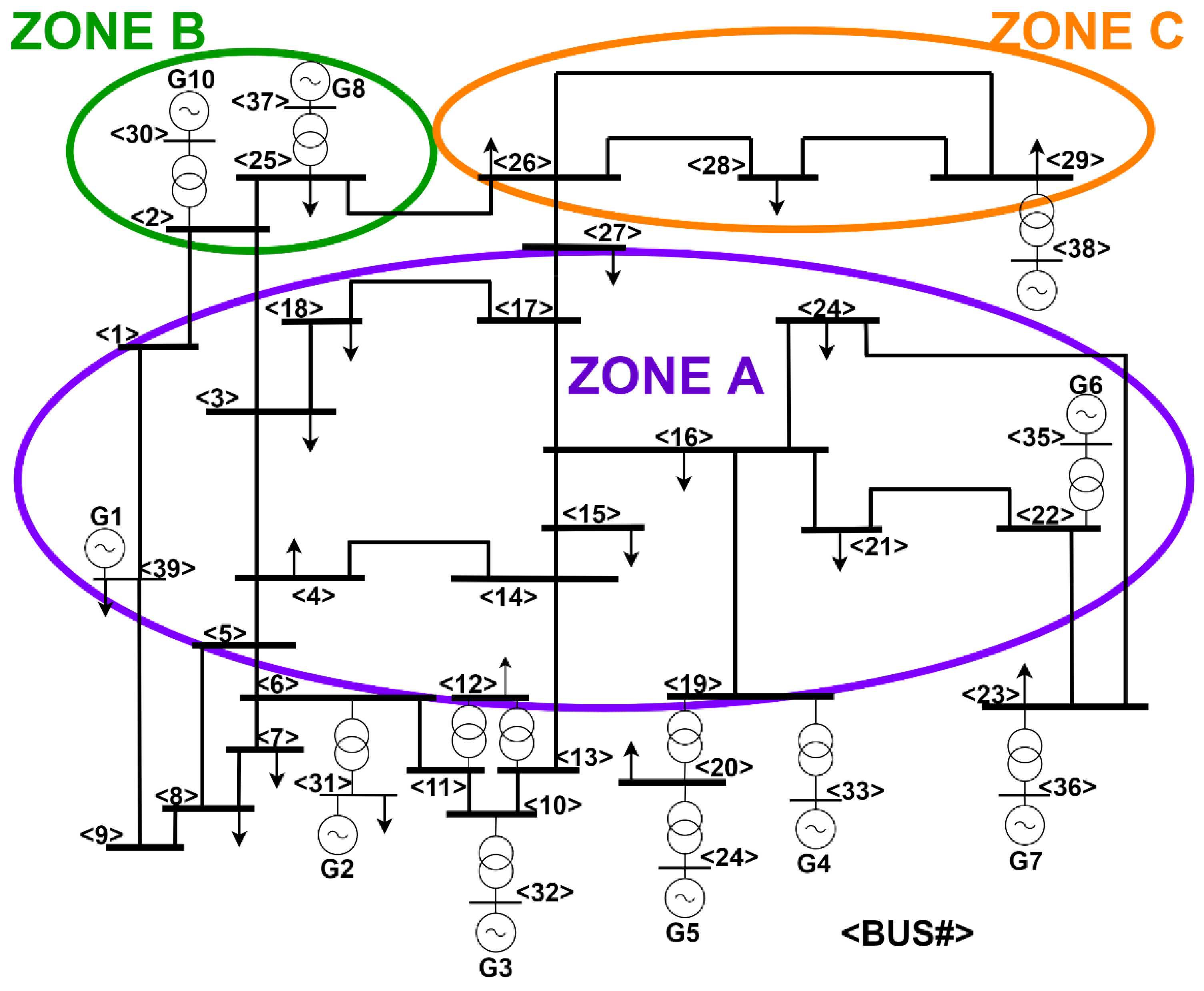
Figure 2 shows the diagram of the IEEE 39-bus power system test case with three zones. In this system, different thresholds are found depending on the area where the disturbance occurs, and it is possible to determine in which plant to carry out the emergency control.
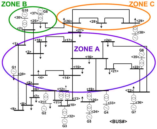
Figure 2.
New England 39-bus power system.
Network security was previously determined during the steady-state operation of each scenario considered in the test. The simulations were carried out using the DIgSILENT POWERFACTORY software, considering the three-phase faults and selecting random locations in the power system. The disturbances were carried out at each iteration, starting at zero seconds (0 s) until it reached the critical clearing time and the corresponding switching of the transmission line, assuming that the sample time was 10 m (Δt = 10 ms) at the update time of the PMUs and using the bus voltage angle where the generators are coupled.
2.7. Offline Calculation of SPS
The calculation of the SPS is based on the zone in which the disturbance occurs and the greater relative angle (AR) of each area. The method of setting up the SPS uses the data of the PMUs and calculates the center of inertia (COI) and the AR of each area in real-time. In the unstable case (the PTRA are exceeded), a control signal is issued (the activation of the SPS) and the control action time is given each time is exceeded. Otherwise (AR < PTRA), the signal is not required.
In practice, generation tripping is commonly performed in single or multiple units [1], and the intention in this research is not to disconnect an entire generation plant; therefore, three equal generation units are assumed in each generation area. Then, the control action consists of tripping a generation unit (33%) from the area each time the post-fault RACKE exceeds the limit, calculated in descending order from the highest to the lowest relative angle of each area. That is, 33% of the following area will be tripped as many times as necessary to control the system and keep the RACKE below the specified limit.
Table 1 shows a matrix with the control signals based on the relative angles and the respective zones that reach higher values in degrees. In this study, the term “C_ #” is the number of orders of the respective control action to be taken in the system.
2.8. Measurement of Synchronized Angular Velocity
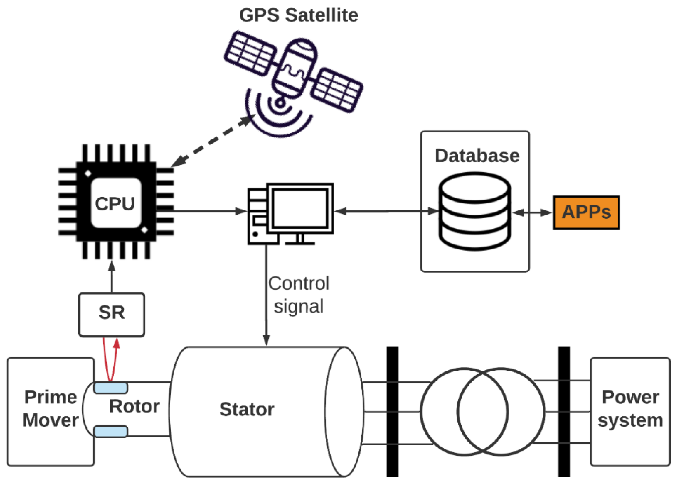
The angular velocity of the synchronous machine is measured directly on the rotor, on which is placed a series of reflective samples that reflect a laser light beam that reflects onto an optical sensor equipped with a Siemens SFH 309 phototransistor, and whose response time is 7 μs [32]. The optical sensor captures the reflected signal and, through a transistorized circuit, the digital pulses are obtained so that the system CPU (Arduino Uno board) computes the angular velocity by executing an algorithm.
For the synchronization of the speed measurement, the PPS generated by the global navigation satellite system (GNSS) is used. This pulse is obtained through a GPS module [31], which, when picked up by the CPU, starts the algorithm for the calculation of the variable of interest with its respective time stamp and sends data using the UDP protocol. This is performed using the W5100 Ethernet Shield designed for the CPU ArduinoUno. The implementation of the measurement system is illustrated in Figure 3.

Figure 3.
The synchronized angular velocity measurement system.
2.9. Algorithm for Synchronization and Angular Velocity Measurement
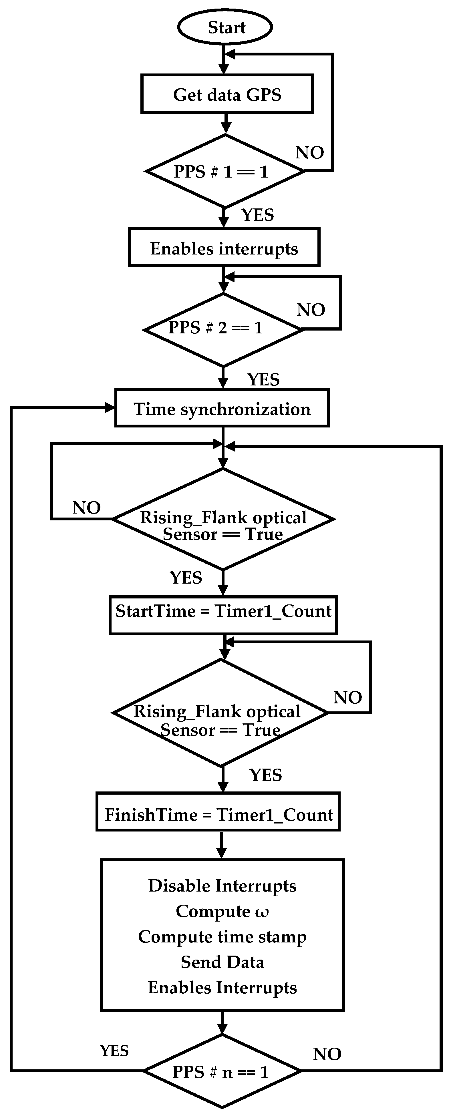
The synchronization and speed measurement algorithm was developed in the Arduino IDE environment based on the C++ programming language, with the characteristics shown in Table 2, and some others found in [33]. The GPS module PPS pin and the optical sensor are connected to pins 2 and 3 of the CPU, to determine the angular velocity using synchronization. Once the PPS is detected, there is an interruption in the Arduino board that enables the calculation of the speed. After the PPS, the CPU waits for the first pulse detected by the optical sensor, at which moment an interruption is generated that starts the calculation of the speed. After obtaining the value of the variable, the synchronized information is transmitted with its respective time stamp and data transmission using the UDP protocol and made using a network board W5100 Ethernet Shield [33]. Figure 4 shows the flowchart diagram of the algorithm implemented to perform the synchronization and speed measurement. After the value of the variable is available, the synchronized information is transmitted. In this algorithm, low-level programming was used to calculate the variable of interest (). For this development, the key was to use the time register in the Arduino Uno CPU (TIMER1). Details about the time frames can be found in [34].
Table 2.
The technical specifications of the Arduino Uno board [33].
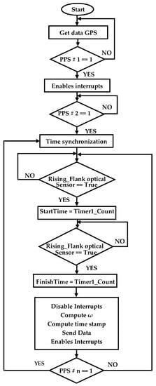
Figure 4.
Flowchart of the algorithm to calculate the synchronized angular velocity.
2.10. Synchronization and Time Stamp
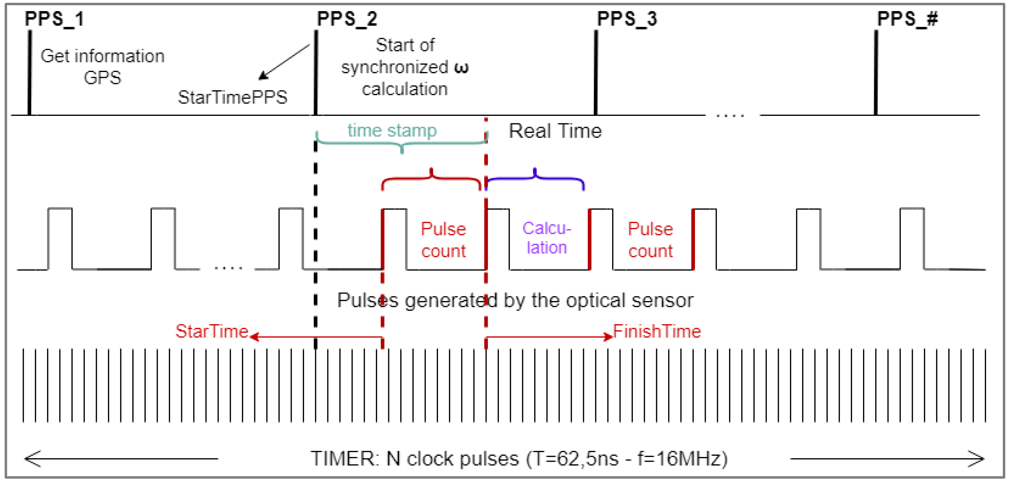
Given the information sent by the GPS (date, hour GTM, length, latitude, PPS, and others), it takes a few hundred milliseconds, and the data is not received every time a PPS is generated. Therefore, this information is received in the first PPS pulse, and the date and time are filtered. Once the data are obtained, time is broken down into respective parts (hours, minutes, and seconds). Moreover, each time a PPS is received, these data are synchronized, increasing the seconds corresponding to the hour. However, a timestamp is necessary for the angular velocity variable, calculated as shown in Equation (11). From PPS_2 (Figure 5), which generates an interruption and activates the angular velocity calculation, the time is synchronized, and the elapsed time is taken by the TIMER1 assigning its value to the variable . Then, following the attainment the respective pulses of the optical sensor (which are used to calculate the angular velocity), a time value is assigned to the variable .
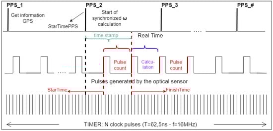
Figure 5.
Synchronization diagram with a timestamp.
Thus, the variable angular velocity will be synchronized because the data will be accompanied by the date and time (h:m:s:ms).
2.11. Calculation of Angular Velocity
The angular velocity is established as expressed in Equation (12):
where represents the angular velocity of the synchronous machine, is the mechanical frequency of the rotor of the synchronous machine, and ρ is the number of pairs of poles. The mechanical frequency is calculated using an algorithm based on the interruptions to determine the angular velocity. At the first interruption (rising edge), after the second PPS is generated by the optical sensor (as shown in Figure 5), the value of TIMER1 is assigned to the variable . Subsequently, at the following interruption (second rising edge), the value of TIMER1 is assigned to the variable . With these two values, the difference in pulses between two successive rising edges of the optical sensor represents the number of pulses () as expressed in Equation (13):
The frequency of the clock used in the CPU is 16 MHz [35]. Therefore, the time between the two pulses is given by Equation (14):
The period corresponding to the course of successive rising edges is then given by Equation (15):
where refers to the period and, with this value, the mechanical frequency can be calculated as expressed in Equation (16):
where NR is the number of reflectors (that generate rising edges) located in the rotor. Thus, the angular velocity is then calculated using Equation (16) applied in Equation (12).
It should be noted that low-level programming was used for the calculation of , which allows greater control over the execution time of the algorithm and reduces the error in the calculation of the variable.
3. Results
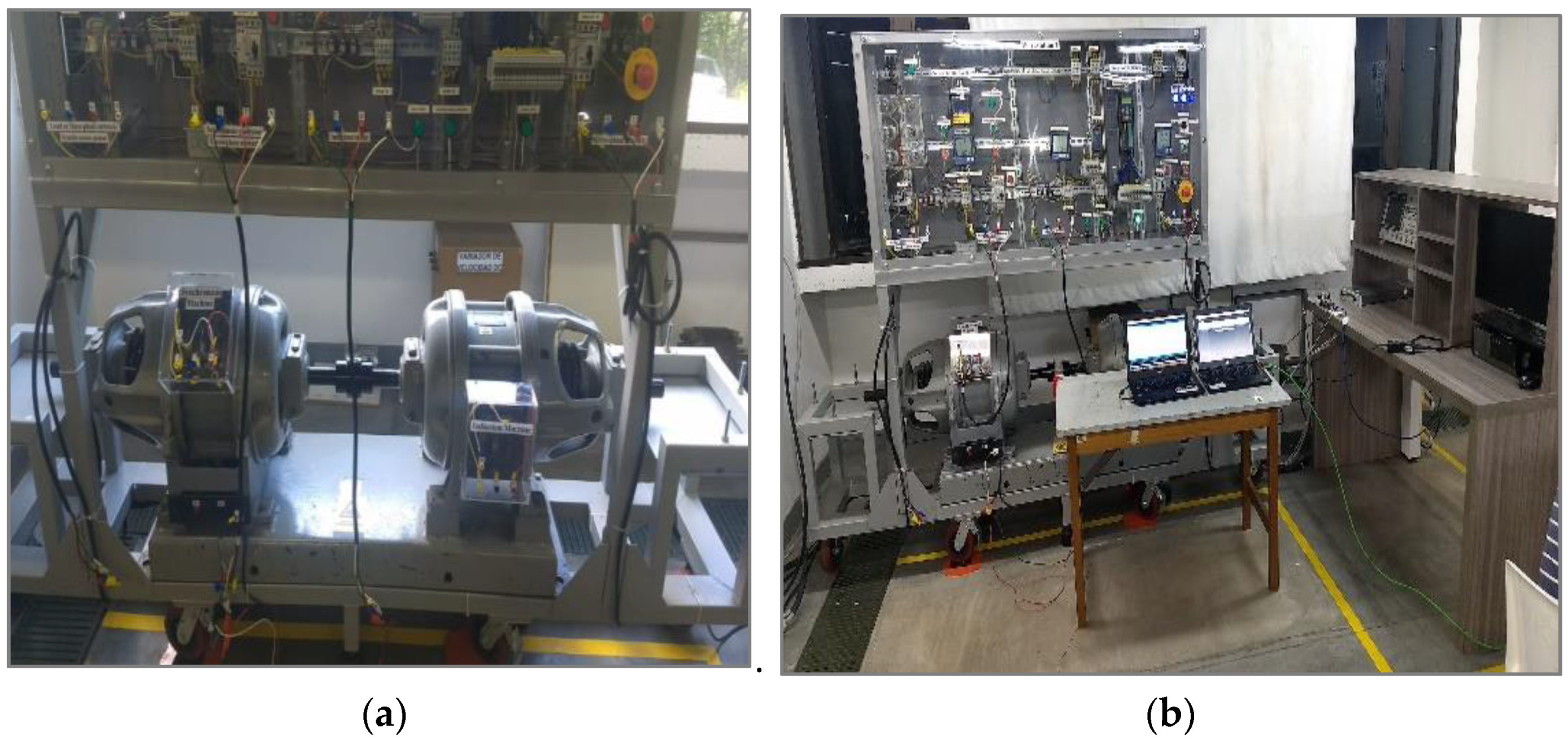
Synchronized angular velocity measurements were performed on a 5 KVA generator at 1200 RPM, as shown in Figure 6a,b. This is a six-pole machine of 60 Hz, driven by an induction motor as the prime mover.
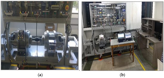
Figure 6.
(a) A synchronous generator of 5 KVA at 1200 RPM and (b) the experiment for the measurement and transmission of information.
Figure 7 shows the experiment for the synchronization of the measurements with their respective CPU and GPS modules. These modules allow for the measurement of the speed of the rotor, the sending of the data to the system that evaluates the stability of the electrical machine, and the obtainment of the PPS from the satellite.
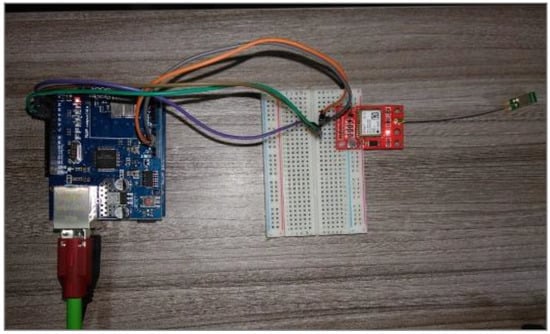
Figure 7.
The GPS module, CPU Arduino Uno, and Shield Ethernet.
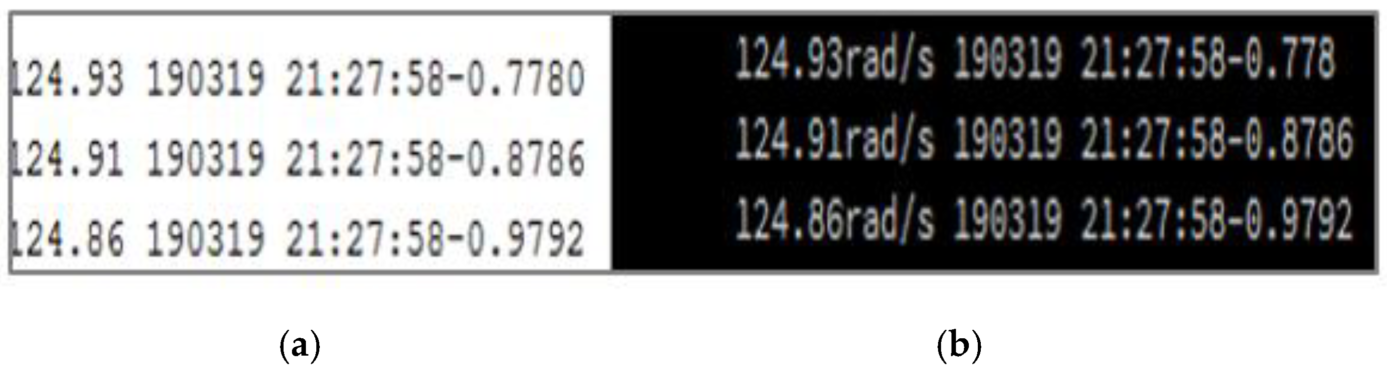
Figure 8 shows a sample of the data received in the processing software environment using the Arduino Uno board, the serial monitor, and the UDP protocol.
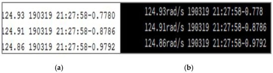
Figure 8.
(a) Information printed from the serial monitor developed using Arduino Uno and (b) data reception in the processing software environment.
The effectiveness of the proposed method is evaluated in the New England IEEE 39-bus power system running dynamic simulations using the DIgSILENT PowerFactory software. This system has 10 generation plants, 39 buses, and 19 loads, and generator 2 is the reference machine. The initial conditions for the dynamic simulations are calculated using power flows that ensure a stable condition before the occurrence of a disturbance. By using the COI index, the power system instability can be predicted. If the system is unstable, the angular velocities and the respective RACKE for each machine and the system can be calculated.
3.1. Case Study 1
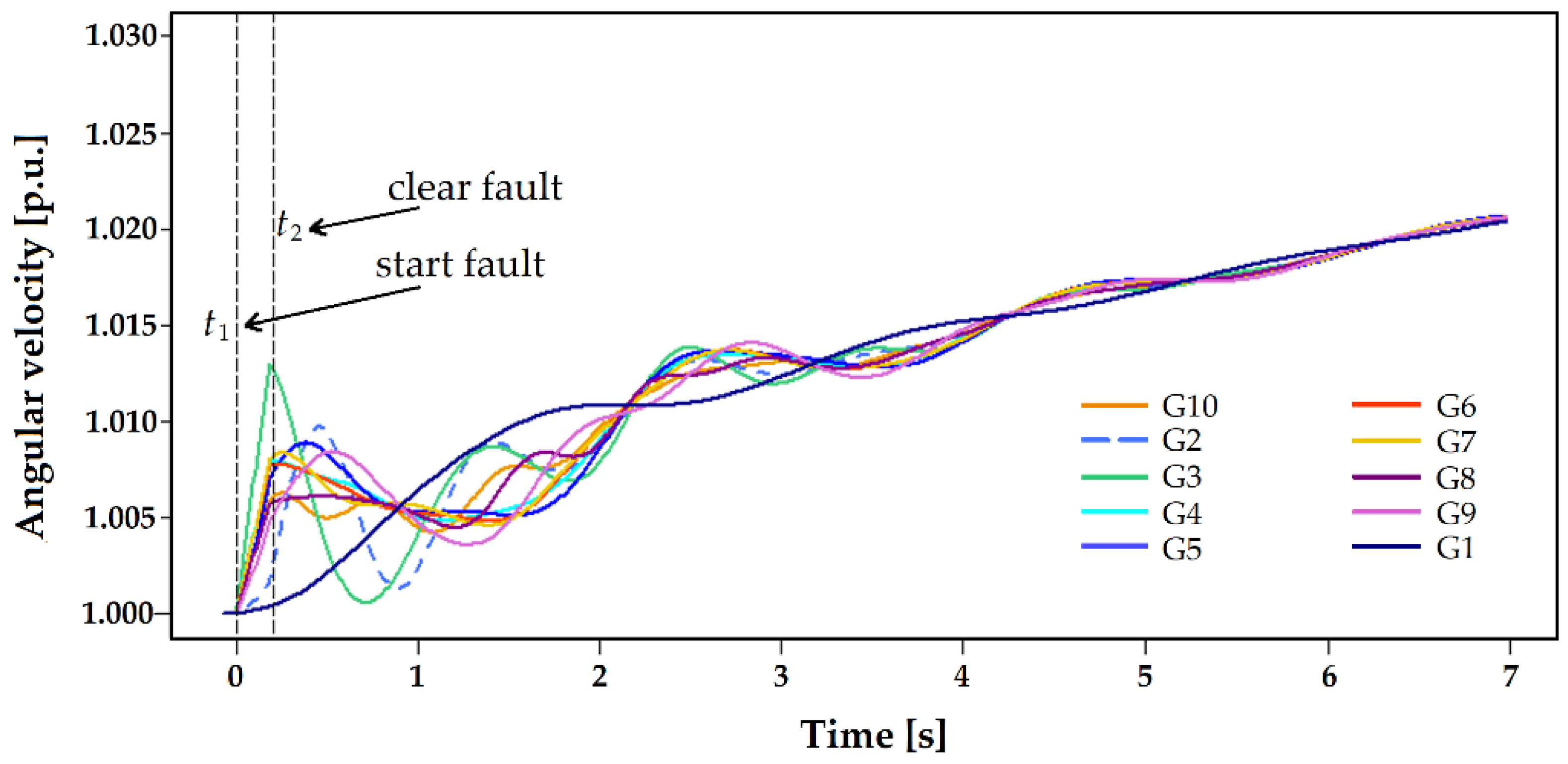
A three-phase fault was evaluated in line 13–14. The fault started at and the clearing time was divided into two times: was the critically stable clearing time (170 ms) and was the fault clearing time for the unstable case (200 ms).
Thus, Figure 9 shows that when the fault is cleared at , the system becomes critical stable; the machines present oscillations at the beginning; and the angular velocity of each rotor increases, searching for a higher operating point, but the system does not lose synchronism.
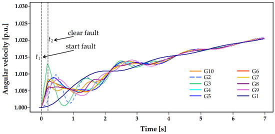
Figure 9.
Rotor speed of the generator in a critical stable case.
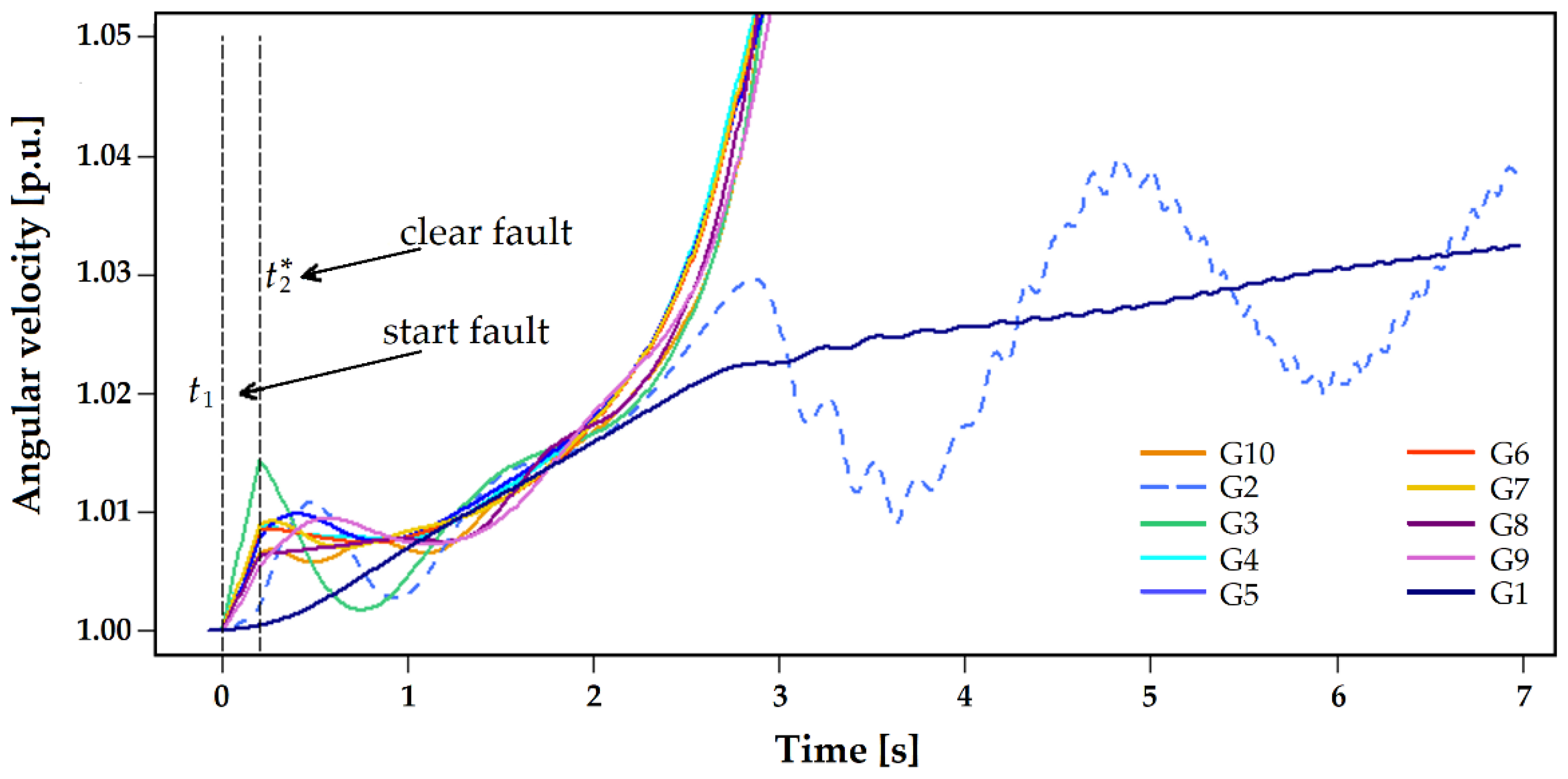
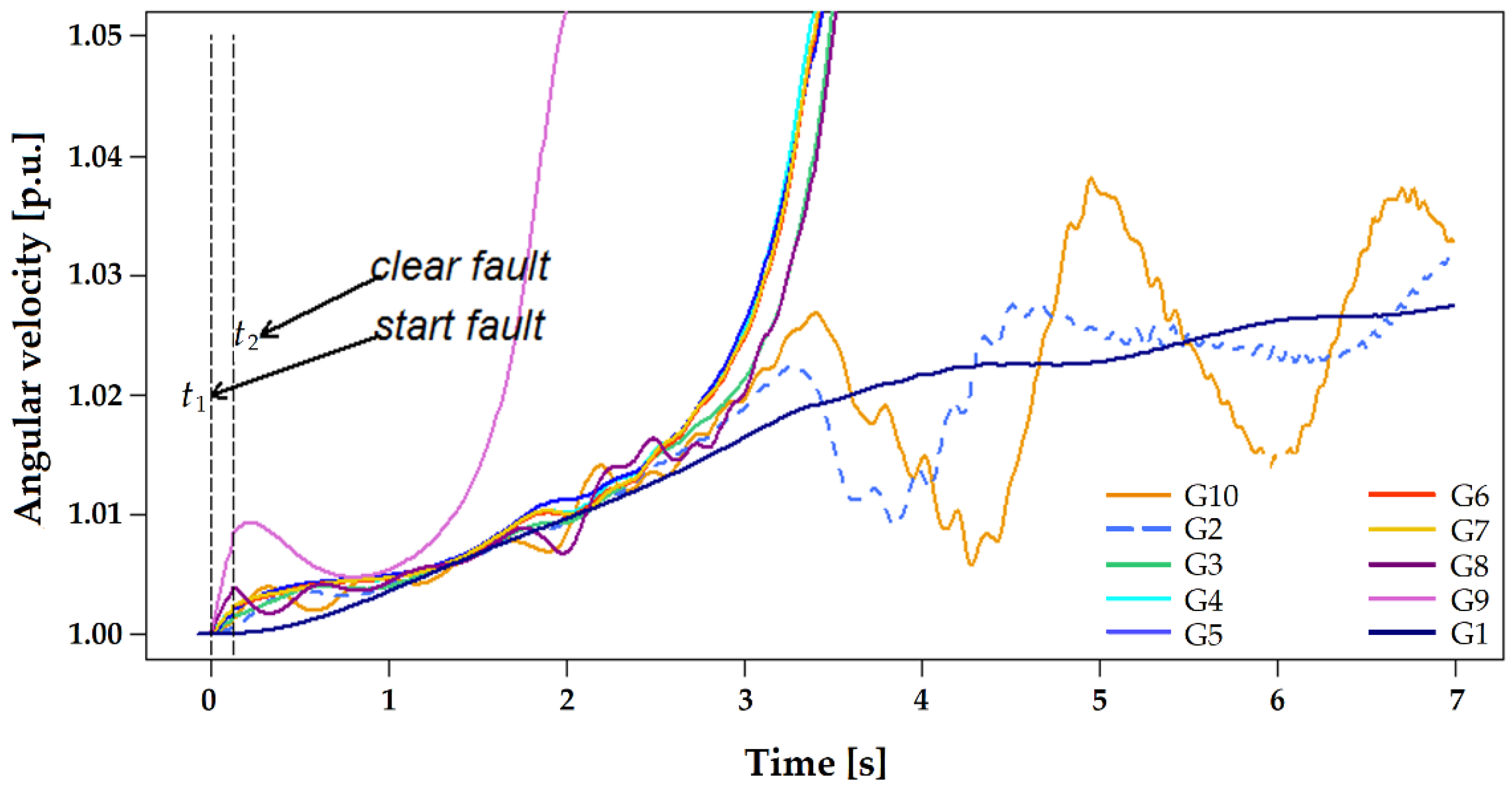
In turn, Figure 10 shows that when the fault is cleared at , taking a longer time to do so than the time , the system becomes unstable after the first oscillation of the machines. In this case, the acceleration is slight and a group of generators causes the system to rapidly become unstable. For both this case and the previous one, the solution is to rapidly determine the moment when the faults must be cleared to avoid system instability.
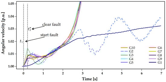
Figure 10.
Rotor speed of the generator in an unstable case.
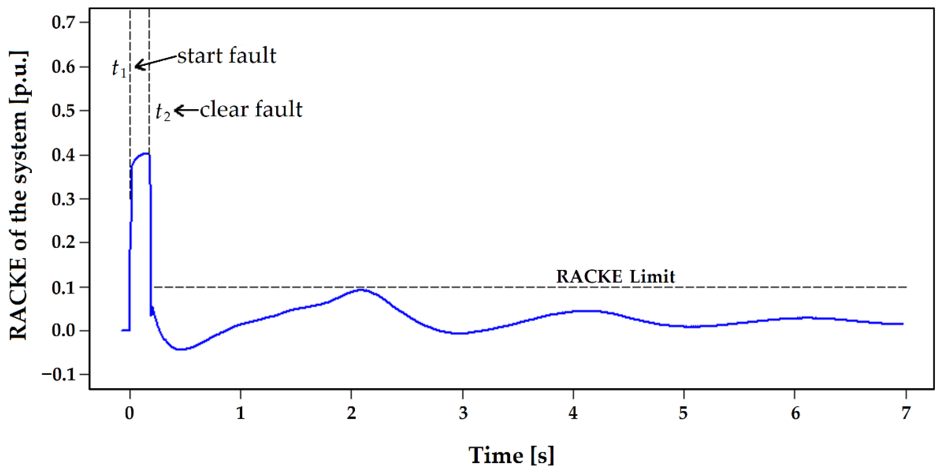
After evaluating the response of the generators, two tests were carefully conducted considering different fault clearance times to evaluate the system using the RACKE and the proposed SPS. For this purpose, the three-phase fault in line 13–14 was simulated, and the angular velocity variable was stored during and after the fault. For = 170 ms (critically stable time) the RACKE is less than the limit of kinetic energy gained by the machines of the system in the post-fault event, showing that, again, the system found a stable point; that is, RACKE < , as shown in Figure 11. This shows how the RACKE of the system (RACKE_SIS) remains a slightly lower than the established limit, and the kinetic energy absorbed by the generators will be delivered back to the system to maintain balance.
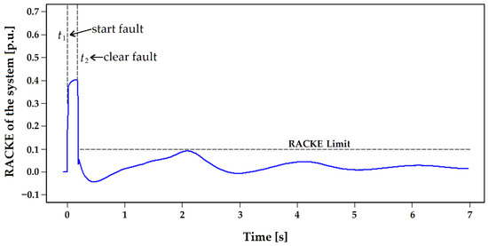
Figure 11.
RACKE_SIS vs. time and the critical stable case.
Figure 12 shows the behavior of the RACKE_SIS for an unstable case of the three-phase fault in line 13–14, when the clearing time is = 200 ms. Note that the RACKE_SIS, during the transient state operation, presents a similar value to the critical stable case presented in Figure 11. However, after the event and the first response, the machines begin to absorb energy rapidly until they collapse. When the curve reaches the limit (RACKE > ), the generators continue to absorb kinetic energy, making them move faster, thus further increasing their kinetic energy. Therefore, a control action must be carried out when this limit is exceeded to dissipate the energy stored by the electrical machines.

Figure 12.
RACKE_SIS vs. time and the unstable case.
Each point of the curve in Figure 12 represents the value of the instantaneous real-time kinetic energy change due to the synchronized measurements of the angular velocity. This result makes it possible to know the exact time at which the control action must be taken. For example, Figure 12 shows that the first control action must be at 1.35 s (1.15 s after the clearing time), and the control action is taken over the generation areas 7 and 5, according to the SPS.
Figure 13 shows the behavior of the RACKE_SIS when the three-phase fault is presented on line 13–14 with a clearing time = 200 ms (unstable case), but considers two control actions, such as, first, reducing the power generation only in G7 and, second, reducing the power generation in G7 and G5, subsequently applying the SPS. The first curve, the light blue line, corresponds to the response of the system without control, showing the unstable system, as previously presented, and requires a reduction of the supplied power to achieve stability. Then, a second curve, the fuchsia line, is the result of considering a control action on G7 (−33% power); however, this action is not enough to solve the problem and the machines continue to absorb kinetic energy, and the limit is exceeded again at 3 s. Finally, a third curve, the dark blue line, is the result of considering a second control action on the generator with the highest AR (G5 with −33% power at 3 s); in this case, the system maintains synchronism (RACKE < ) and the kinetic energy absorbed by each machine is delivered to the system. Therefore, with this last control action, the stability of the system is guaranteed.

Figure 13.
RACKE_SIS vs. time, with and without control.
3.2. Case Study 2
In this case, a three-phase fault in line 26–28 (zone C) is carried out at . Then, the fault is cleared at 100 ms, tripping the line simultaneously. Thus, Figure 14 shows that the angular velocity of each machine rotor increases after the first oscillation. After three seconds, the oscillation is reduced and the angular velocity continues to increase, looking for a higher operating point, whilst maintaining stability at any instant of the post-fault event.
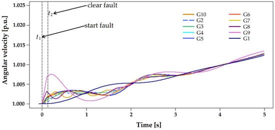
Figure 14.
Rotor speed of generators with a fault in line 26–28.
Likewise, the kinetic energy change criterion is computed in the three-phase fault in line 26–28, which is shown in Figure 15. When the fault occurs at 0, the RACKE starts increasing and reaches the highest value of the event. Then, when the fault is cleared at 100 ms and the line is tripped, the RACKE decreases to the lowest limit values and starts oscillating. The RACKE maintains oscillation during the first 4 s and then it shows stabilization. The result shows that the system maintains stability during the studied period. Effectively, it is noted how the threshold is not reached at any instant of the post-fault event.
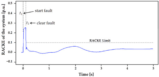
Figure 15.
RACKE_SIS vs. time and the critical case of stability.
Similarly, a three-phase fault with a duration of 130 ms is evaluated with the same initial conditions of line 26–28 (zone C). In this case, the line is removed again to clear the fault. Although the system does not present a loss of synchronism during the first oscillation, the system collapse will occur in a subsequent one, as shown in Figure 16. The result shows that the clearing time is long enough for the system to neither recover nor maintain stability. Generator G9 is the first to present a higher oscillation in time and it accelerates after the first oscillation, being the first to lose its synchronism. During the following two seconds, the majority of the generators continue accelerating to higher values and require some control actions to avoid damage. Only three generators continue to oscillate after the 3.5 s and search for a new operating point; however, in this condition, the system will probably go into a blackout.
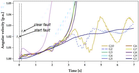
Figure 16.
RACKE_SIS vs. time and without control.
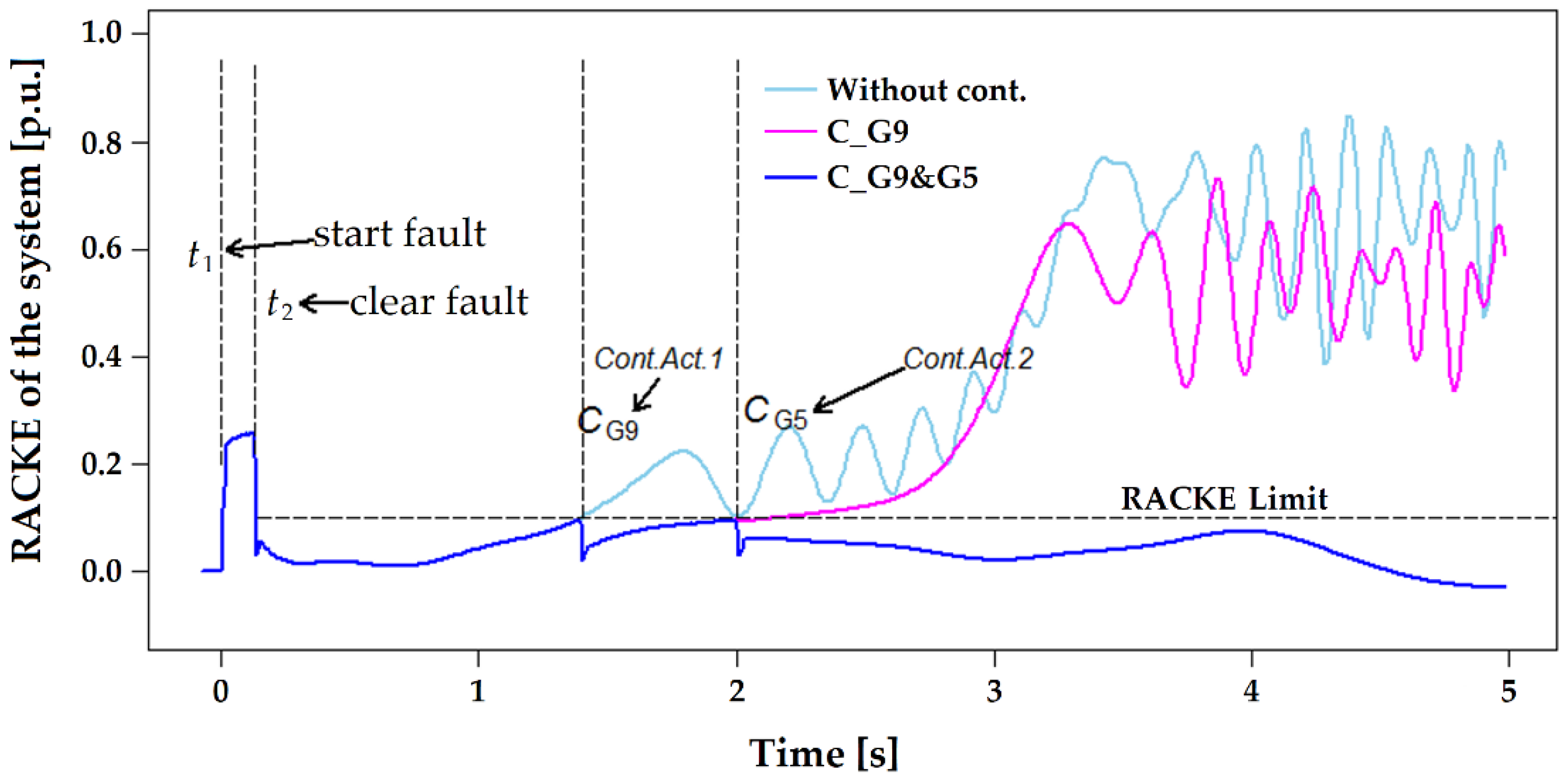
Figure 17 shows the behavior of the RACKE when a three-phase fault in line 26–28 (zone C) is simulated and the fault is cleared at = 130 ms (unstable case), but considers two control actions with the use of the SPS described in Section 2, such as, first, reducing the power generation only in G9 and, second, reducing the power generation in G5. The first curve, the light blue line, corresponds to the response of the system without control, showing that the system is unstable and requires a reduction of the supplied power to achieve stability. The result shows that the RACKE exceeds the limit (1.4 s) and control actions are required to maintain stability.
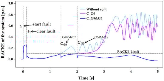
Figure 17.
RACKE_SIS vs. time, with and without control.
Then, a second curve, the fuchsia line, is the result of considering control actions of 33%, power tripped at 1.4 s in area 9 (Zone C); however, this action is not enough to solve the problem and the machines continue to absorb kinetic energy and the limit is exceeded, again, at around 2 s.
Finally, a third curve, the dark blue line, is the result of considering a control action on a second generator (G5 with −33% power at 2 s), according to SPS; in this case, the system maintains synchronism (RACKE < ) and the kinetic energy is absorbed by each of the machines and, subsequently, this energy is delivered back into the system. Therefore, with this last control action, the stability of the system is guaranteed.
4. Conclusions
This research proposed a method to evaluate and alleviate transient stability in a real-time operation, through the synchronized angular velocity of the power system’s machines. An attached power system and the kinetic energy change criterion can represent the dynamics of a multi-machine power system by projecting and calculating energy. This provides an intuitive measure of the precise instant in which a control action must be taken by integrating measurements of the WAMS system in conjunction with offline simulations, which allow the reliable assembly of an SPS. The results obtained by the simulations demonstrate the effectiveness of the proposed method and the SPS. The criterion shows that the method is fast enough because the calculation does not depend on the network structure and does not need detailed information about the system model. In addition, the identification of coherent groups of generators is not necessary. More important is the implementation of the measurement system, which only depends on one variable, in this case, the synchronized angular velocity. Low-level programming was used to calculate the interest variable, which allows greater control over the execution time of the algorithm and reduces the error in the calculation. Although the measurement was obtained experimentally using a single machine, the method can be scalable to large multi-machine systems. It is recommended that each machine uses an Arduino Uno board, an optical sensor, and a communication board, to communicate with the satellite and to synchronize the measurement. Therefore, a more real condition can be applied in future analyses. Furthermore, the board used in the experiments shows that the method allows the synchronization of measurements, and another board can be used with PTP protocol to improve synchronization.
Author Contributions
Conceptualization, A.F.D.-A.; methodology, A.F.D.-A.; validation, J.E.C.-B.; formal analysis, A.F.D.-A., A.D.-P. and J.E.C.-B.; investigation, A.F.D.-A., A.D.-P. and J.E.C.-B.; writing—original draft preparation, A.F.D.-A.; writing—review and editing, A.F.D.-A., A.D.-P. and J.E.C.-B. All authors have read and agreed to the published version of the manuscript.
Funding
This research received no external funding.
Institutional Review Board Statement
Not applicable.
Informed Consent Statement
Not applicable.
Data Availability Statement
Not applicable.
Acknowledgments
This work was supported by the Universidad Nacional de Colombia, Sede Medellín. We thank the Department of Electrical Engineering and Automation, Facultad de Minas, for the continuous support of our research. Albert Deluque-Pinto thanks the project “Transformation Strategy for Colombian energy sector on the 2030 horizon”, awarded by call 788 of MinCiencias (Scientific Ecosystem Program), contract number FP44842-210-2018.
Conflicts of Interest
The authors declare no conflict of interest.
References
- Bhui, P.; Senroy, N. Real time prediction and control of transient stability using transient energy function. IEEE Trans. Power Syst. 2016, 32, 923–934. [Google Scholar] [CrossRef]
- Wehenkel, L.; Pavella, M. Preventive vs. emergency control of power systems. In Proceedings of the IEEE PES Power Systems Conference and Exposition, New York, NY, USA, 10–13 October 2004; pp. 628–633. [Google Scholar]
- Ernst, D.; Pavella, M. Closed-loop transient stability emergency control. In Proceedings of the 2000 IEEE Power Engineering Society Winter Meeting. Conference Proceedings (Cat. No.00CH37077), Singapore, 23–27 January 2000; Volume 1, pp. 58–62. [Google Scholar]
- Stagg, G.; El-Abiad, A. Computer Methods in Power System Analysis; McGraw-Hill: New York, NY, USA, 1968; pp. 366–397. [Google Scholar]
- Fouad, A.A.; Vittal, V. Power System Transient Stability Analysis Using the Transient Energy Function Method; Prentice Hall: Hoboken, NJ, USA, 1992; ISBN 013682675X. [Google Scholar]
- Pai, M.A. Energy Function Analysis for Power System Stability; Springer: Boston, MA, USA, 1989; ISBN 978-1-4612-8903-6. [Google Scholar]
- Aghamohammadi, M.R.; Tabandeh, S.M. A new approach for online coherency identification in power systems based on correlation characteristics of generators rotor oscillations. Int. J. Electr. Power Energy Syst. 2016, 83, 470–484. [Google Scholar] [CrossRef]
- Jahromi, M.Z.; Kouhsari, S.M. A novel recursive approach for real-time transient stability assessment based on corrected kinetic energy. Appl. Soft Comput. 2016, 48, 660–671. [Google Scholar] [CrossRef]
- Al-Taee, A.A.; Al-Taee, M.A.; Al-Nuaimy, W. Augmentation of transient stability margin based on rapid assessment of rate of change of kinetic energy. Electr. Power Syst. Res. 2016, 140, 588–596. [Google Scholar] [CrossRef]
- Ota, H.; Kitayama, Y.; Ito, H.; Fukushima, N.; Omata, K.; Morita, K.; Kokai, Y. Development of transient stability control system (TSC system) based on on-line stability calculation. IEEE Trans. Power Syst. 1996, 11, 1463–1472. [Google Scholar] [CrossRef]
- Pavella, M.; Ernst, D.; Ruiz-Vega, D. Transient Stability of Power Systems: A Unified Approach to Assessment and Control; Kluwer Academic Publishers: Boston, MA, USA, 2000; ISBN 0792379632. [Google Scholar]
- Dasgupta, S.; Paramasivam, M.; Vaidya, U.; Ajjarapu, V. PMU-based model-free approach for real-time rotor angle monitoring. IEEE Trans. Power Syst. 2015, 30, 2818–2819. [Google Scholar] [CrossRef]
- Sun, K.; Lee, S.T.; Zhang, P. An adaptive power system equivalent for real-time estimation of stability margin using phase-plane trajectories. IEEE Trans. Power Syst. 2011, 26, 915–923. [Google Scholar] [CrossRef]
- Wang, H.; Zhang, B.; Hao, Z. Response based emergency control system for power system transient stability. Energies 2015, 8, 13508–13520. [Google Scholar] [CrossRef] [Green Version]
- Sajadi, A.; Preece, R.; Milanović, J. Identification of transient stability boundaries for power systems with multidimensional uncertainties using index-specific parametric space. Int. J. Electr. Power Energy Syst. 2020, 123, 106152. [Google Scholar] [CrossRef]
- Shabani, H.R.; Kalantar, M. Real-time transient stability detection in the power system with high penetration of DFIG-based wind farms using transient energy function. Int. J. Electr. Power Energy Syst. 2021, 133, 107319. [Google Scholar] [CrossRef]
- Bang, H.; Aryani, D.R.; Song, H. Application of battery energy storage systems for relief of generation curtailment in terms of transient stability. Energies 2021, 14, 3898. [Google Scholar] [CrossRef]
- Amraee, T.; Ranjbar, S. Transient instability prediction using decision tree technique. IEEE Trans. Power Syst. 2013, 28, 3028–3037. [Google Scholar] [CrossRef]
- Haidar, A.M.A.; Mustafa, M.W.; Ibrahim, F.A.F.; Ahmed, I.A. Transient stability evaluation of electrical power system using generalized regression neural networks. Appl. Soft Comput. 2011, 11, 3558–3570. [Google Scholar] [CrossRef]
- Tiwari, S.; Naresh, R.; Jha, R. Neural network predictive control of UPFC for improving transient stability performance of power system. Appl. Soft Comput. 2011, 11, 4581–4590. [Google Scholar] [CrossRef]
- Gomez, F.R.; Rajapakse, A.D.; Annakkage, U.D.; Fernando, I.T. Support vector machine-based algorithm for post-fault transient stability status prediction using synchronized measurements. IEEE Trans. Power Syst. 2011, 26, 1474–1483. [Google Scholar] [CrossRef]
- Moulin, L.S.; da Silva, A.P.A.; El-Sharkawi, M.A.; MarksII, R.J. Support vector machines for transient stability analysis of large-scale power systems. IEEE Trans. Power Syst. 2004, 19, 818–825. [Google Scholar] [CrossRef] [Green Version]
- Rahmatian, M.; Chen, Y.C.; Palizban, A.; Moshref, A.; Dunford, W.G. Transient stability assessment via decision trees and multivariate adaptive regression splines. Electr. Power Syst. Res. 2017, 142, 320–328. [Google Scholar] [CrossRef]
- AI-Taee, M.A.; AI-Azzawi, F.J.; Al-Taee, A.A.; Al-Jumaily, T.Z. Real-time assessment of power system transient stability using rate of change of kinetic energy method. IEE Proc.-Gener. Transm. Distrib. 2001, 148, 505. [Google Scholar] [CrossRef]
- Kong, X.; Jia, H.; Jiang, Y.; Zhao, S.; Fang, D. Criterion to evaluate power system online transient stability based on adjoint system energy function. IET Gener. Transm. Distrib. 2015, 9, 104–112. [Google Scholar] [CrossRef]
- Kundur, P. Power System Stability and Control; McGraw-Hill: New York, NY, USA, 1994; p. 1176. [Google Scholar]
- Kimbark, E. Power System Stability. Vol. 1, 1st ed.; Wiley: New York, NY, USA, 1948. [Google Scholar]
- Sherwood, M.; Dongchen, H.; Venkatasubramanian, V.M. Real-time detection of angle instability using synchrophasors and action principle. In Proceedings of the 2007 iREP Symposium—Bulk Power System Dynamics and Control—VII. Revitalizing Operational Reliability, Charleston, SC, USA, 19–24 August 2007; pp. 1–11. [Google Scholar]
- Zamani, M.A.; Beresh, R.; Cress, S.L. A PMU-augmented stability power limit assessment for reliable arming of special protection systems. Electr. Power Syst. Res. 2015, 128, 134–143. [Google Scholar] [CrossRef]
- Diaz-Alzate, F.A.; Candelo-Becerra, E.J.; Villa Sierra, F.J. Transient stability prediction for real-time operation by monitoring the relative angle with predefined thresholds. Energies 2019, 12, 838. [Google Scholar] [CrossRef] [Green Version]
- Shi, F.; Zhang, H.; Xue, G. Instability prediction of the inter-connected power grids based on rotor angle measurement. Int. J. Electr. Power Energy Syst. 2017, 88, 21–32. [Google Scholar] [CrossRef]
- Siemens Semiconductor Group. SFH309 Datasheet. Available online: https://pdf1.alldatasheet.es/datasheet-pdf/view/45639/SIEMENS/SFH309.html (accessed on 28 August 2021).
- Arduino Ethernet Shield V1. Available online: https://www.arduino.cc/en/Main/ArduinoEthernetShieldV1 (accessed on 28 August 2021).
- ATMEL Corporation. Data Sheet ATmega328P. Available online: https://pdf1.alldatasheet.es/datasheet-pdf/view/1132281/ATMEL/ATMEGA328P.html (accessed on 28 August 2021).
- Arduino Uno Rev3. Available online: https://store-usa.arduino.cc/products/arduino-uno-rev3/ (accessed on 28 August 2021).

Publisher’s Note: MDPI stays neutral with regard to jurisdictional claims in published maps and institutional affiliations. |
© 2021 by the authors. Licensee MDPI, Basel, Switzerland. This article is an open access article distributed under the terms and conditions of the Creative Commons Attribution (CC BY) license (https://creativecommons.org/licenses/by/4.0/).