
Modeling Wind Speed Based on Fractional Ornstein-Uhlenbeck Process

 ,
,  , ,
, ,  ,
,  and
and 
Abstract
:1. Introduction
- −
- Probability Density Function (PDF) describing the statistical distribution of wind speeds that depend on the specific site and used to estimate potential energy production [4].
- −
- Autocorrelation Function (ACF) that shows the strength of the relationship between two successive values of the same time series [5]. Its accurate modeling is necessary to improve the reliability of forecasting wind speed fluctuations over short time intervals.
- −
- Systematic daily and seasonal cycles [6] which significantly affect the performance of wind turbines [7] and whose modeling is necessary to predict electricity generation [8]; analyze the aerodynamic interaction between wind turbines in wind farms [9]; and coordinate the operation modes of hybrid RES-based power supply systems.
2. Literature Review
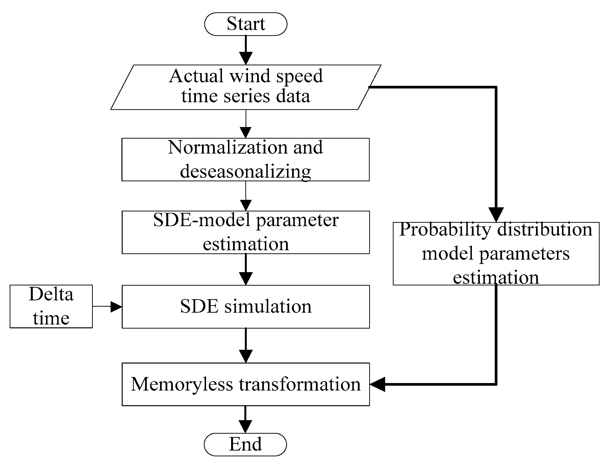
3. Methods and Algorithms
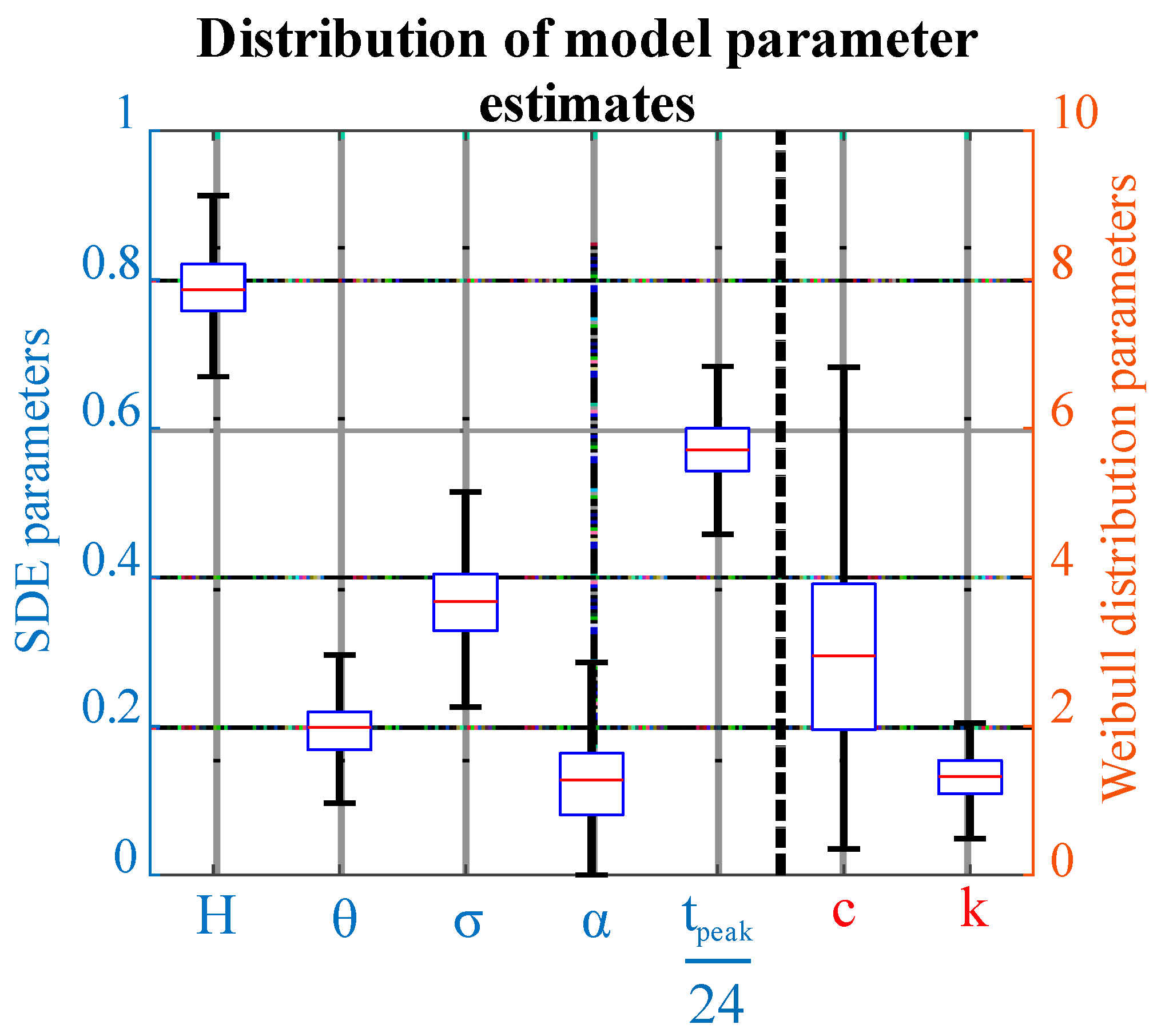
4. Model Parameters Estimation
4.1. Hurst Exponent Estimator
4.2. Diffusion Parameter Estimator
4.3. Mean-Reversion Rate Estimator
4.4. Estimation Parameters of Periodic Function of Daily Pattern
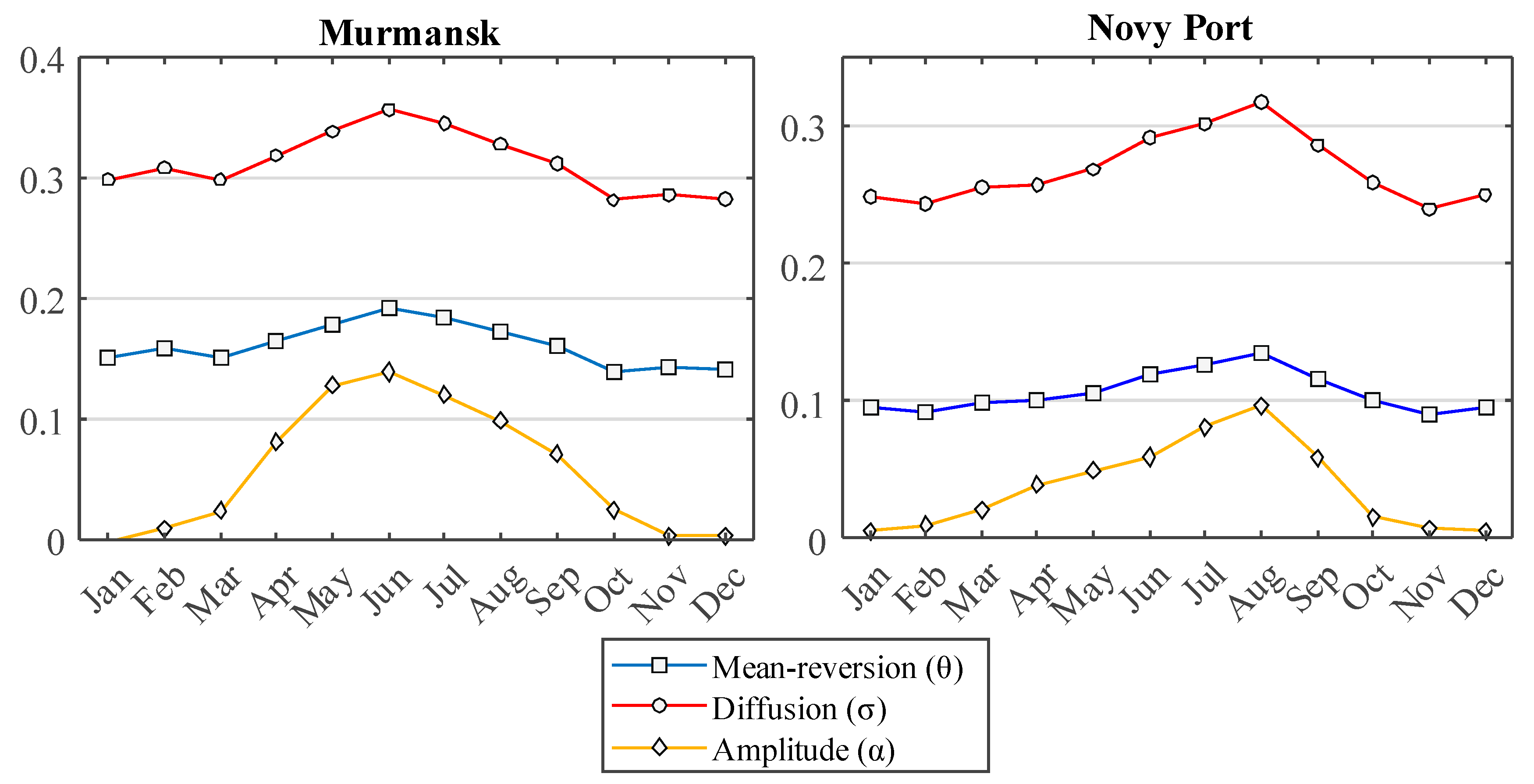
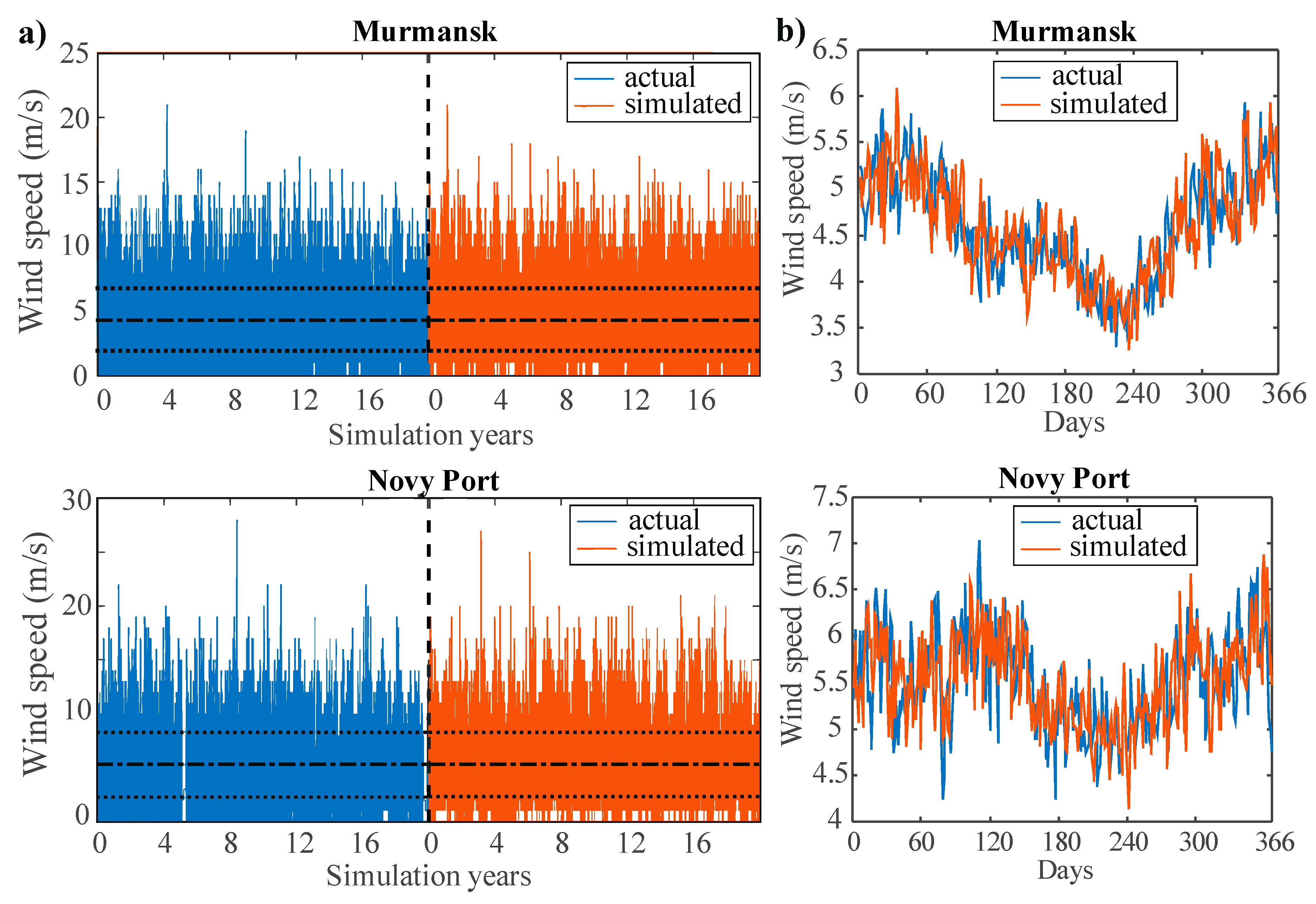
5. Model Validation and Results
6. Conclusions
Author Contributions
Funding
Institutional Review Board Statement
Informed Consent Statement
Data Availability Statement
Conflicts of Interest
Nomenclature
| SDE | Stochastic differential equation |
| Probability density function | |
| ACF | Autocorrelation function |
| RES | Renewable energy source |
| AR | Autoregressive model |
| MA | Moving-average model |
| ARMA | Autoregressive moving-average model |
| GA | Genetic algorithm |
| PSO | Particle swarm optimization |
| fBm | Fractional Brownian motion |
| DP | Daily profile |
| AIC | Akaike information criterion |
| BIC | Bayesian information criterion |
| θ | Mean-reversion rate |
| μ | Long-run mean |
| σ | Diffusion |
| Fractional Brownian motion (c параметрoм Херста ) | |
| α | daily wind speed amplitude parameter |
| tpeak | hour of daytime peak wind speed |
| delta time | |
| cumulative distribution function of Normal distribution | |
| inverse cumulative distribution function |
References
- Choi, Y.; Lee, C.; Song, J. Review of renewable energy technologies utilized in the oil and gas industry. Int. J. Renew. Energy Res. 2017, 7, 592–598. [Google Scholar]
- Goryunov, O.A.; Nazarova, Y.A. Prospects for wind driven power plants application for power supply to the gas industry facilities in the Far North regions. Oil Gas Territ. 2015, 12, 146–150. Available online: https://tng.elpub.ru/jour/article/viewFile/246/247.pdf (accessed on 25 June 2021).
- Vasenin, A.B.; Kryukov, O.V. Issues of electricity supply for route facilities of the Unified Gas Supply system in Russia. Nauchno-Tekhnicheskij Sb. Vesti Gazov. Nauk. 2020, 2, 181–192. Available online: https://cyberleninka.ru/article/n/voprosy-elektropitaniya-vdoltrassovyh-obektov-edinoy-sistemy-gazosnabzheniya-rossii (accessed on 30 July 2021).
- Jung, C.; Schindler, D. Wind speed distribution selection—A review of recent development and progress. Renew. Sustain. Energy Rev. 2019, 114, 109290. [Google Scholar] [CrossRef]
- Brett, A.C.; Tuller, S.E. The autocorrelation of hourly wind speed observation. J. Appl. Meteorol. Climatol. 1991, 30, 823–833. [Google Scholar] [CrossRef] [Green Version]
- Fortuna, L.; Nunnari, G.; Nunnari, S. Nonlinear Modeling of Solar Radiation and Wind Speed Time Series; Springer: Cham, Switzerland, 2016; p. 98. [Google Scholar] [CrossRef]
- Tian, L.; Song, Y.; Zhao, N.; Shen, W.; Wang, T.; Zhu, C. Numerical investigations into the idealized diurnal cycle of atmospheric boundary layer and its impact on wind turbine’s power performance. Renew Energy 2020, 145, 419–427. [Google Scholar] [CrossRef]
- Baker, R.W.; Walker, S.N.; Wade, J.E. Annual and seasonal variations in mean wind speed and wind turbine energy production. Sol. Energy 1990, 45, 285–289. [Google Scholar] [CrossRef]
- Chanprasert, W.; Sharma, R.; Cater, J.; Norris, S. Seasonal variability of offshore wind turbine wakes. In Proceedings of the 22nd Australasian Fluid Mechanics Conference AFMC2020, Brisbane, QLD, Australia, 7–10 December 2020. [Google Scholar] [CrossRef]
- Ghofrani, M.; Alolayan, M. Time series and renewable energy forecasting. In Time Series Analysis and Applications; Mohamudally, N., Ed.; IntechOpen: London, UK, 2018; pp. 77–92. [Google Scholar] [CrossRef] [Green Version]
- Bazionis, I.K.; Georgilakis, P.S. Review of deterministic and probabilistic wind power forecasting: Models, methods, and future research. Electricity 2021, 2, 11–47. [Google Scholar] [CrossRef]
- Elwan, A.A.; Habibuddin, M.H. Statistical approach for wind speed forecasting using markov chain modelling as the probabilistic model. In Proceedings of the 2019 IEEE 2nd International Conference on Power and Energy Applications (ICPEA), Singapore, 27–30 April 2019; pp. 177–182. [Google Scholar] [CrossRef]
- Neshat, M.; Nezhad, M.M.; Abbasnejad, E.; Mirjalili, S.; Tjernberg, L.B.; Garcia, D.A.; Alexander, B.; Wagner, M. A deep learning-based evolutionary model for short-term wind speed forecasting: A case study of the Lillgrund offshore wind farm. Energy Convers. Manag. 2021, 236, 114002. [Google Scholar] [CrossRef]
- Viet, D.T.; Phuong, V.V.; Duong, M.Q.; Tran, Q.T. Models for short-term wind power forecasting based on improved artificial neural network using particle swarm optimization and generic algorithms. Energies 2020, 13, 2873. [Google Scholar] [CrossRef]
- Duan, J.; Zuo, H.; Bai, Y.; Duan, J.; Chang, M.; Chen, B. Short-term wind speed forecasting using recurrent neural networks with error correction. Energy 2021, 217, 119397. [Google Scholar] [CrossRef]
- Wang, J.Q.; Du, Y.; Wang, J. LSTM based long-term energy consumption prediction with periodicity. Energy 2020, 197, 117197. [Google Scholar] [CrossRef]
- Zárate-Miñano, R.; Anghel, M.; Milano, F. Continuous wind speed models based on stochastic differential equations. Appl. Energy 2013, 104, 42–49. [Google Scholar] [CrossRef]
- Arenas-López, J.P.; Badaoui, M. The Ornstein-Uhlenbeck process for estimating wind power under a memoryless transformation. Energy 2020, 213, 118842. [Google Scholar] [CrossRef]
- Iversen, E.B.; Morales, J.M.; Møller, J.K.; Madsen, H. Short-term probabilistic forecasting of wind speed using stochastic differential equations. Int. J. Forecast. 2016, 32, 981–990. [Google Scholar] [CrossRef]
- Ibe, O.C. Markov Processes for Stochastic Modeling, 2nd ed.; Elsevier: Amsterdam, The Netherlands, 2013; p. 514. [Google Scholar] [CrossRef]
- Biagini, F.; Hu, Y.; Øksendal, B.; Zhang, T. Stochastic Calculus for Fractional Brownian Motion and Applications; Springer: London, UK, 2008; p. 330. [Google Scholar] [CrossRef]
- Alaton, P.; Djehiche, B.; Stillberger, D. On modelling and pricing weather derivatives. Appl. Math. Financ. 2002, 9, 1–20. [Google Scholar] [CrossRef]
- Lysy, M.; Pillai, N.S. Statistical Inference for Stochastic Differential Equations with Memory. Available online: https://arxiv.org/abs/1307.1164v1 (accessed on 11 December 2019).
- Perrin, E.; Harba, R.; Jennane, R.; Iribarren, I. Fast and exact synthesis for 1-D fractional Brownian motion and fractional Gaussian noises. IEEE Signal Process. Lett. 2002, 9, 382–384. [Google Scholar] [CrossRef]
- Taqqu, M.S.; Teverovsky, V.; Willinger, W. Estimators for long-range dependence: An empirical study. Fractals 1995, 3, 785–798. [Google Scholar] [CrossRef]
- Su, Y.; Wang, Y. Parameter estimation for fractional diffusion process with discrete observations. J. Funct. Spaces 2019, 9036285. [Google Scholar] [CrossRef] [Green Version]
- Xiao, W.; Zhang, W.; Xu, W. Parameter estimation for fractional Ornstein–Uhlenbeck processes at discrete observation. Appl. Math. Model. 2011, 35, 4196–4207. [Google Scholar] [CrossRef]
- Specializirovannye Massivy Dlya Klimaticheskih Issledovanij. Vserossijskij Nauchno Issledovatel’skij Institut Gidrometeorologicheskoj Informacii-Mirovoj Centr Dannyh (VNIIGMI-MCD) [Specialized Arrays for Climatic Research. All-Russian Research Institute of Hydrometeorological Information (RIHMI-WDC)]. Available online: http://aisori-m.meteo.ru (accessed on 21 March 2019).
- Wilks, D.S. Statistical Methods in the Atmospheric Sciences/D.S. Wilks, 2nd ed.; Elsevier: Amsterdam, The Netherlands, 2006; Volume 649, p. 36. [Google Scholar]
- Burnham, K.P.; Anderson, D.R. Model Selection and Multimodel Inference: A Practical Information-Theoretic Approach, 2nd ed.; Springer: New York, NY, USA, 2002; p. 488. [Google Scholar] [CrossRef] [Green Version]
- Alattar, A.H.; Selem, S.I.; Metwally, H.M.B.; Ibrahim, A.; Aboelsaud, R.; Tolba, M.A.; El-Rifaie, A.M. Performance enhancement of micro grid system with SMES storage system based on mine blast optimization algorithm. Energies 2019, 12, 3110. [Google Scholar] [CrossRef] [Green Version]


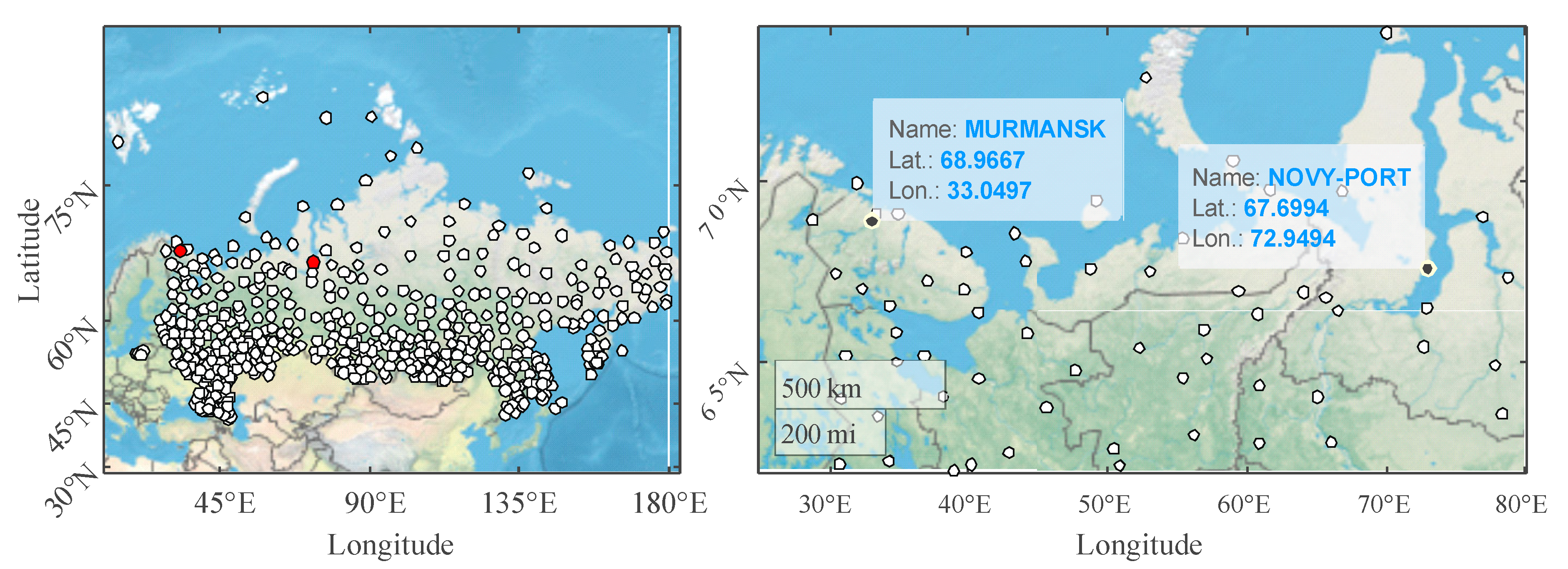
| # | WMO ID | Weather Station | Lat., dd | Lon., dd | Altitude, m | Time Range | Wind Speed Statistic, m/s | |||||
|---|---|---|---|---|---|---|---|---|---|---|---|---|
| Start | End | Δt, h | Min | Max | Mean | std | ||||||
| 1 | 22113 | Murmansk | 68.97 | 33.05 | 57 | 1 January 1999 | 1 January 2019 | 3 | 0 | 21 | 4.58 | 2.56 |
| 2 | 23242 | Novy Port | 67.70 | 72.95 | 12 | 0 | 28 | 5.50 | 3.13 | |||
| Weather Station | Observed Data | Standard Model (H = 1/2) | Fractional Model (H > 1/2) | |||||||||
|---|---|---|---|---|---|---|---|---|---|---|---|---|
| Min | Max | Mean | Std | Min | Max | Mean | Std | Min | Max | Mean | Std | |
| Δt = 3 | ||||||||||||
| 1 | 0 | 21 | 4.58 | 2.56 | 0.01 | 20.25 | 4.58 | 2.55 | 0.01 | 20.67 | 4.58 | 2.55 |
| 2 | 0 | 28 | 5.50 | 3.13 | 0.01 | 25.53 | 5.50 | 3.13 | 0.01 | 26.11 | 5.50 | 3.13 |
| Δt = 1 | ||||||||||||
| 1 | 0 | 21 | 4.58 | 2.56 | 0.01 | 21.06 | 4.58 | 2.55 | 0 | 20.75 | 4.58 | 2.55 |
| 2 | 0 | 28 | 5.50 | 3.13 | 0.01 | 26.81 | 5.50 | 3.13 | 0 | 26.36 | 5.50 | 3.13 |
| Criterion | Standard Model (H = 1/2) | Fractional Model (H > 1/2) | ||||||
|---|---|---|---|---|---|---|---|---|
| Min | Max | Mean | Std | Min | Max | Mean | Std | |
| Δt = 3 | ||||||||
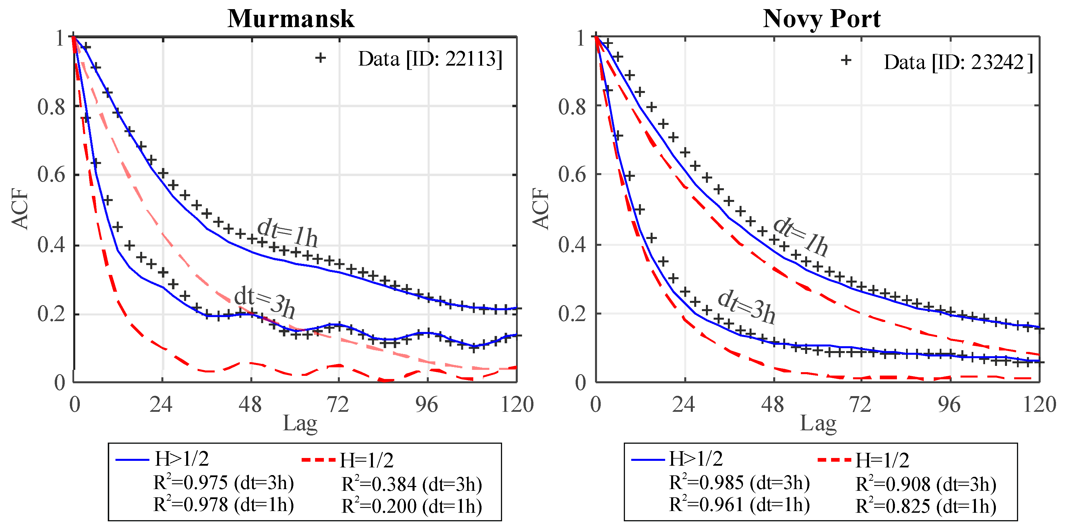
| R2 (ACF) | 0 | 0.9780 | 0.4675 | 0.2679 | 0.3928 | 0.9931 | 0.9327 | 0.0632 |
| R2 (DP) | 0.0167 | 0.9947 | 0.9027 | 0.1263 | 0.0506 | 0.9962 | 0.9201 | 0.0994 |
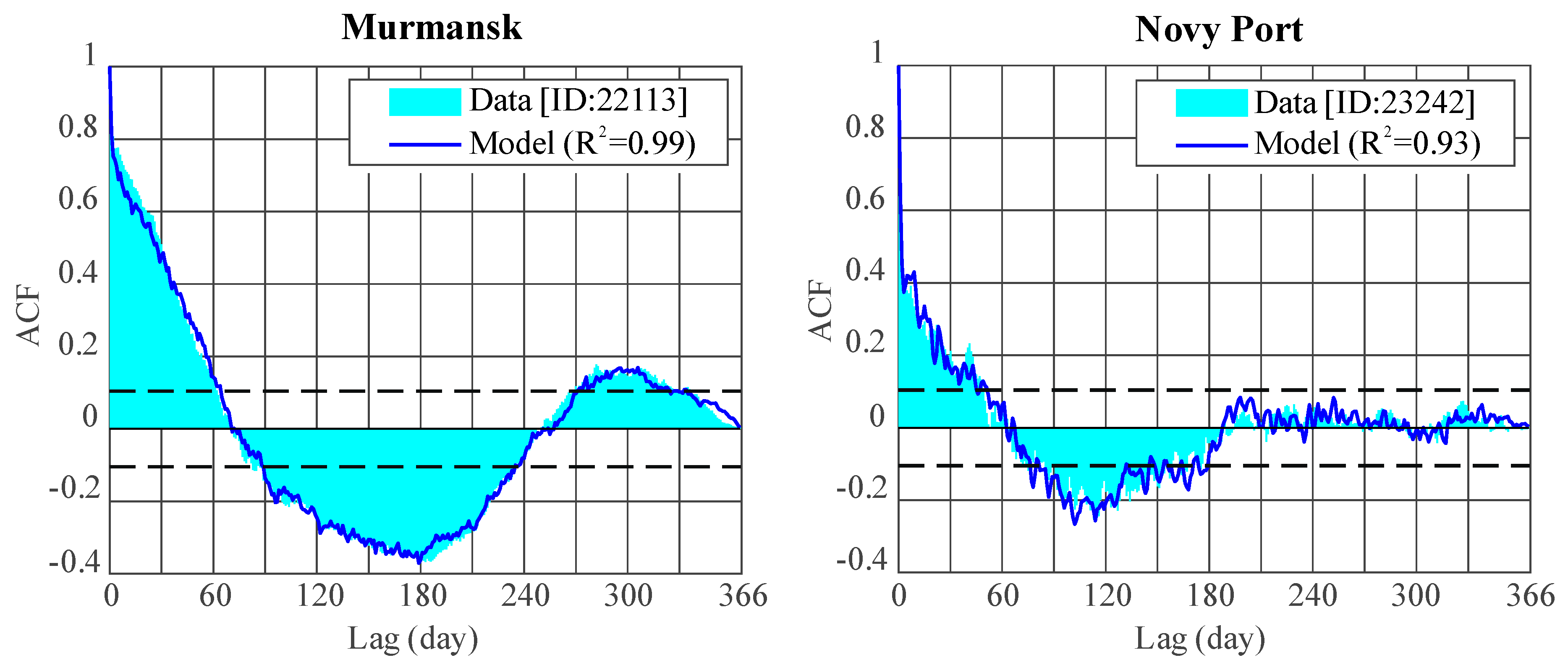
| R2 (Daily ACF) | 0.5894 | 0.9997 | 0.9784 | 0.0437 | 0.7121 | 0.9996 | 0.9848 | 0.0310 |
| R2 (PDF) | 0.6445 | 0.9954 | 0.9432 | 0.0444 | 0.6372 | 0.1171 | 0.9432 | 0.0446 |
| AIC(1 × 10⁻³) | 36.727 | 520.165 | 238.049 | 83.621 | 23.451 | 519.740 | 236.995 | 84.217 |
| BIC(1 × 10⁻³) | 38.27 | 521.708 | 239.588 | 83.624 | 25.016 | 521.304 | 238.555 | 84.220 |
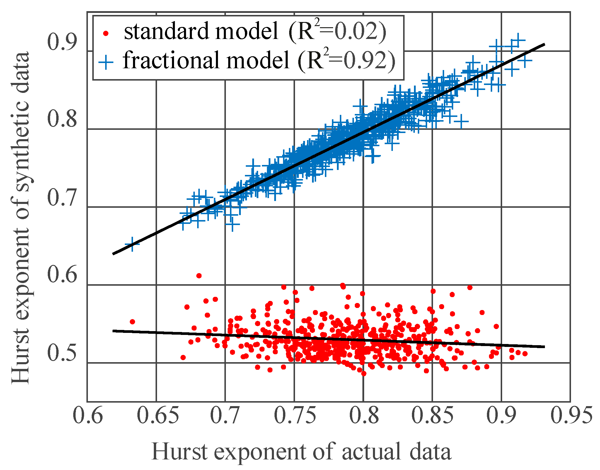
| R2 (H) | 0.0210 | 0.9215 | ||||||
| Δt = 1 | ||||||||
| R2 (ACF) | 0 | 0.9899 | 0.3137 | 0.2732 | 0 | 0.9967 | 0.9110 | 0.1000 |
| R2 (DP) | 0.0641 | 0.9899 | 0.8858 | 0.1193 | 0.0641 | 0.9933 | 0.9187 | 0.0959 |
| R2 (Daily ACF) | 0.6782 | 0.9997 | 0.9827 | 0.0374 | 0.7506 | 0.9995 | 0.9843 | 0.0290 |
| R2 (PDF) | 0.6371 | 0.9956 | 0.9436 | 0.0446 | 0.6804 | 0.9957 | 0.9436 | 0.0438 |
| AIC(1 × 10⁻³) | 36.730 | 1549.40 | 696.113 | 255.202 | 14.964 | 1550.40 | 689.560 | 257.190 |
| BIC(1 × 10⁻³) | 38.432 | 1551.10 | 697.810 | 255.205 | 16.689 | 1552.10 | 691.281 | 257.193 |
| R2 (H) | 0.0151 | 0.9056 | ||||||
Publisher’s Note: MDPI stays neutral with regard to jurisdictional claims in published maps and institutional affiliations. |
© 2021 by the authors. Licensee MDPI, Basel, Switzerland. This article is an open access article distributed under the terms and conditions of the Creative Commons Attribution (CC BY) license (https://creativecommons.org/licenses/by/4.0/).
Share and Cite
Obukhov, S.; Ahmed, E.M.; Davydov, D.Y.; Alharbi, T.; Ibrahim, A.; Ali, Z.M. Modeling Wind Speed Based on Fractional Ornstein-Uhlenbeck Process. Energies 2021, 14, 5561. https://doi.org/10.3390/en14175561
Obukhov S, Ahmed EM, Davydov DY, Alharbi T, Ibrahim A, Ali ZM. Modeling Wind Speed Based on Fractional Ornstein-Uhlenbeck Process. Energies. 2021; 14(17):5561. https://doi.org/10.3390/en14175561
Chicago/Turabian StyleObukhov, Sergey, Emad M. Ahmed, Denis Y. Davydov, Talal Alharbi, Ahmed Ibrahim, and Ziad M. Ali. 2021. "Modeling Wind Speed Based on Fractional Ornstein-Uhlenbeck Process" Energies 14, no. 17: 5561. https://doi.org/10.3390/en14175561
APA StyleObukhov, S., Ahmed, E. M., Davydov, D. Y., Alharbi, T., Ibrahim, A., & Ali, Z. M. (2021). Modeling Wind Speed Based on Fractional Ornstein-Uhlenbeck Process. Energies, 14(17), 5561. https://doi.org/10.3390/en14175561