1. Introduction
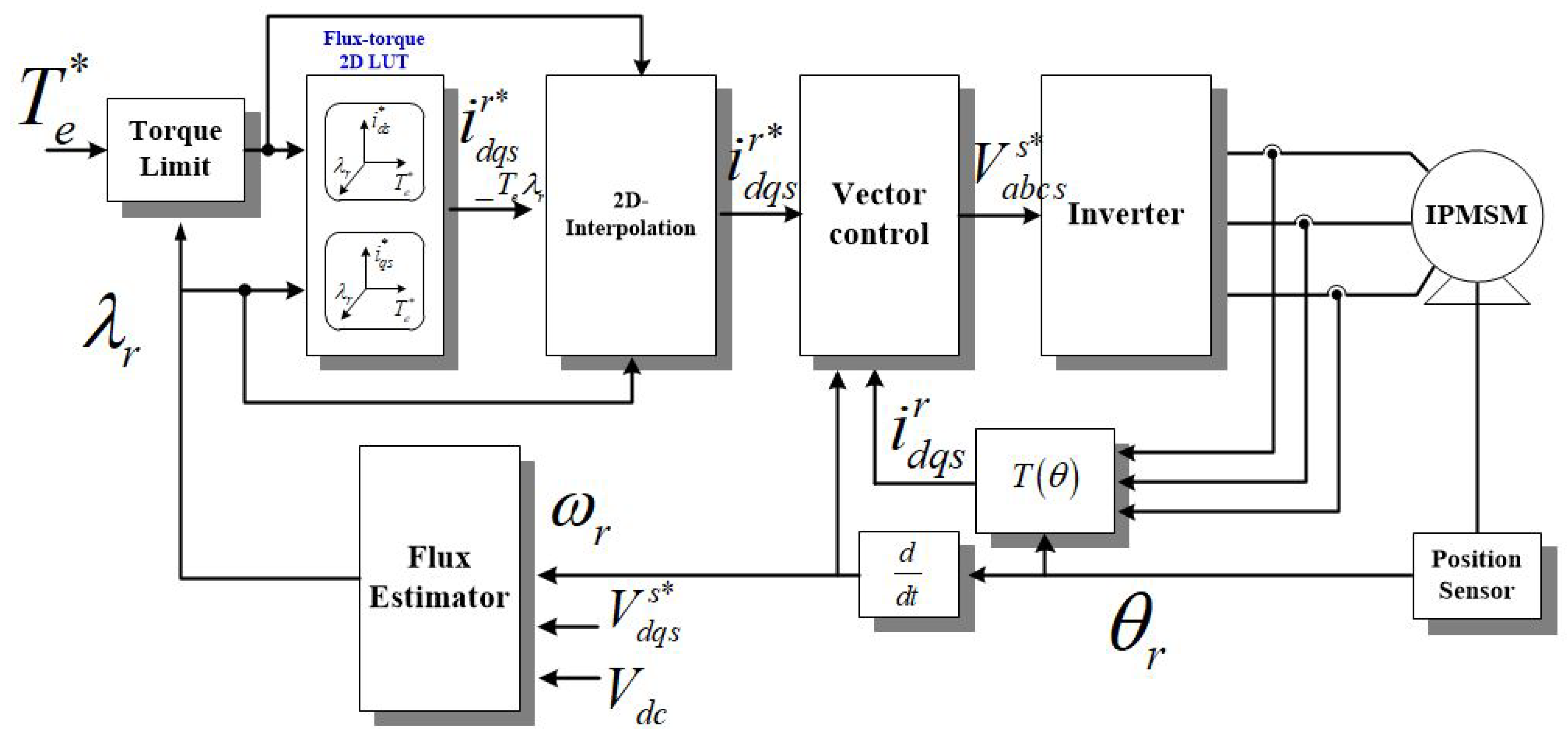
The permanent magnet synchronous motor (PMSM) application range has gradually broadened in recent years through automotive motor control, producing higher output than conventional motors. This type of automotive motor control requires robust control based on the input parameters. Consequently, the look-up table-based PMSM torque control method is used to generate current commands with two different parameters. As shown in
Figure 1 [
1], among these control methods, the flux-torque two-dimensional look-up table (2D-LUT)-based torque control method is commonly used owing to the DC-link voltage variation. However, suitable current references for all operating circumstances cannot be stored in memory. Because of inherent memory restriction, the current references can only be stored in the memory by a specific fixed unit; therefore, the outputs of the look-up table have discrete characteristics despite the continuous input parameters.
Owing to these problems, motor control systems that generate current commands in look-up tables use 2D interpolation. 2D-LUT with 2D-interpolation is applied not only for traction motor drives of Hybrid Electric Vehicle(HEV) [
2] and Electric Vehicle(EV) [
3], actuator driver for automotive systems [
4], but also for many other PMSM-based applications [
5,
6]. Additionally, there exist other table-based methods besides the aforementioned current command method, such as the voltage–vector table [
7], current angle table [
8], 3D-LUT-based control method [
9]. However, those other table-based methods are not as popular as the two-dimensional current-command-based table as a result of the simple concept and easy implementation of the two-dimensional current table. Two-dimensional interpolation changes the discrete data stored in the 2D-LUT into linear data and outputs them. When a parameter is an input, the output of the data stored in the memory is calculated using a linear interpolation method called first-order Newton interpolation [
10,
11].
If the amount of data stored in the LUT used for PMSM control is sufficient, the interpolation error caused by the linear interpolation of the current command generated by the 2D interpolation is very small and can be ignored. However, when the amount of data in the LUT is insufficient, the interpolation error generated by linear interpolation is large, and the interpolation error cannot be ignored, especially in the high-speed operating region. In automotive applications, the system uses a large amount of memory space for system safety function and failure diagnosis, the memory space allocated for the LUT is usually insufficient.
Studies have been conducted to optimize memory to solve this insufficient memory problem. The method proposed in [
12,
13] recreates the current commands of the LUT based on system data. Therefore, the number of memories can be reduced based on the operating conditions. In the optimization method proposed in [
14,
15], the curve-fitting method was used to reduce memory. However, all the methods introduced above require the exact PMSM parameters. Because the parameters of PMSM vary depending on the temperature, speed, etc., the effect of the memory optimization method is limited. Conversely, [
16,
17] provide a method for applying a counter-electromotive force table to compensate for the interpolation error. Although these methods require additional experiments to create a counter-electromotive force table, they can not only significantly reduce the current reference memory but also be robust to parameter variation. However, since this kind of method has a slow response and the current commands are incorrect when the voltage error is small, additional compensation is required. In [
18], an additional feedforward compensation method is proposed in order to improve the performance of interpolation error compensation, proposed in [
17], based on the voltage error. However, even with this method, the additional compensation was not effective when the value of the voltage error was small, and the q-axis current response was not fast enough when the reference current changed very fast.
This paper proposes an improved interpolation error compensation method. In this study, a voltage feedforward controller and a current feedforward controller are added to the interpolation error compensator proposed in [
17,
18]. The proposed algorithm was verified experimentally based on a motor-generator setup in laboratory. In the experiment, the proposed method is compared with the conventional 2D-Interpolation-based method to verify its performance during the maximum power control in the field weakening operation region. Additionally, experimental results between the proposed feedforward controllers are compared. One of the experiment results is when only the voltage feedforward controller is applied to the PI controller, and another one is when two proposed feedforward controllers are fully applied.
2. Conventional Compensation Method for 2D-Interpolation
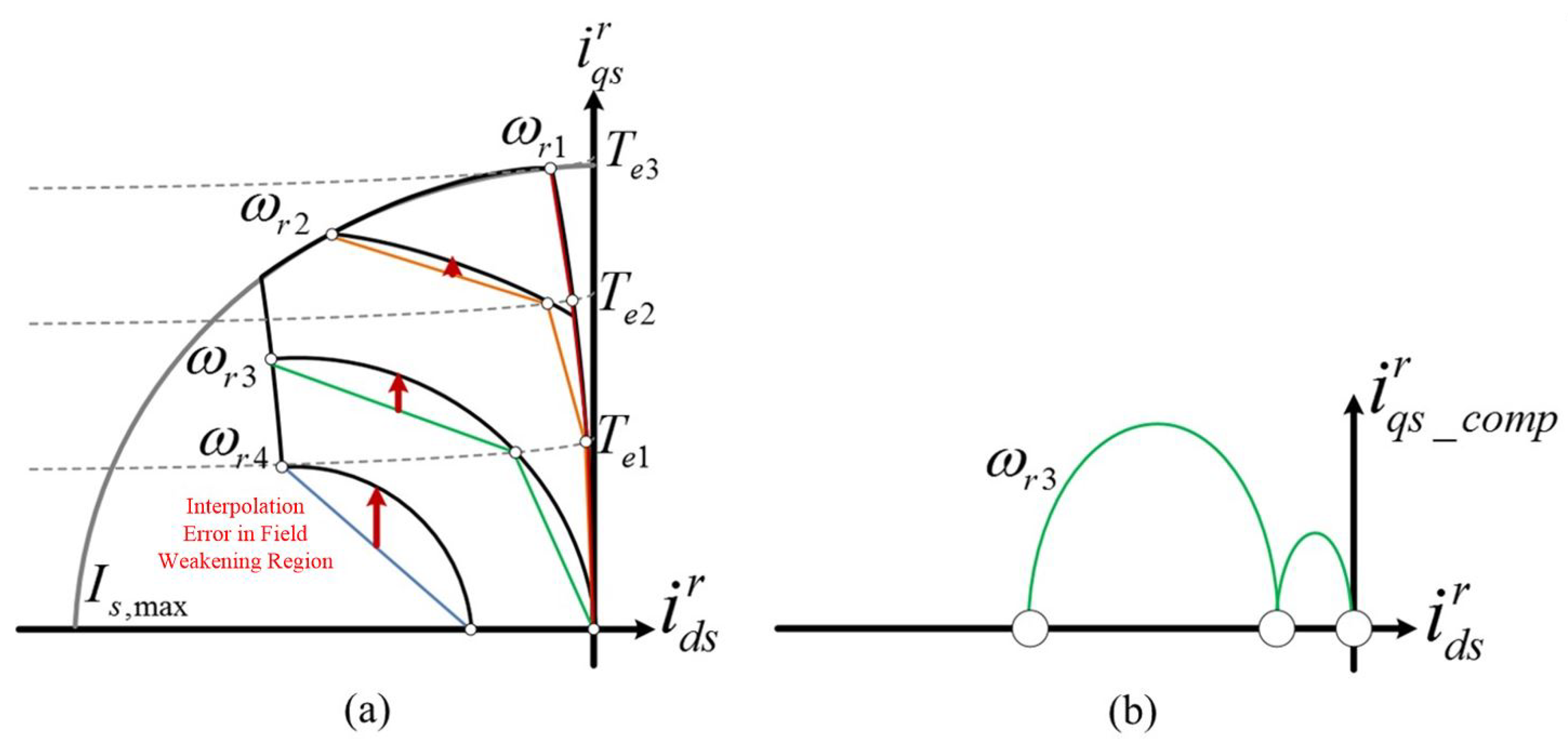
Figure 2a shows the interpolation error in the field weakening operation region [
17]. The 2D-Interpolation method generates a linear interpolated output using the equation described in Equation (
1).
In 2D-Interpolation, the stored adjacent dq-axis current references are connected linearly. Although it can reduce the error better than using only the look-up table output, the generated power is lower than the capable maximum power. This is because the number of LUT data for corresponding motor speed are different since the maximum torque output varies according to the motor speed. For example, in the case of
and
, there are four data points in LUT, 3 points for
, and 2 points for
respectively. As described in arrows in
Figure 2a, the smaller number of data points for the corresponding speed causes more error in the interpolation.
To calculate the maximum power control current trajectory, the fundamental PMSM model equations are:
The output torque is as follows.
To achieve maximum power operation, the operating current must reach the required voltage and current. In the field weakening operation region, the increasing current trajectory should follow the voltage limit ellipse. The current trajectory can be obtained as follows, assuming that resistance is ignored:
Under the constant torque operation region, voltage limitation does not affect the operating current; therefore, in this region, the voltage magnitude from the generated current and speed must be considered at each torque and speed to prevent divergence of current. The stored voltage magnitude was obtained experimentally using the following equation:
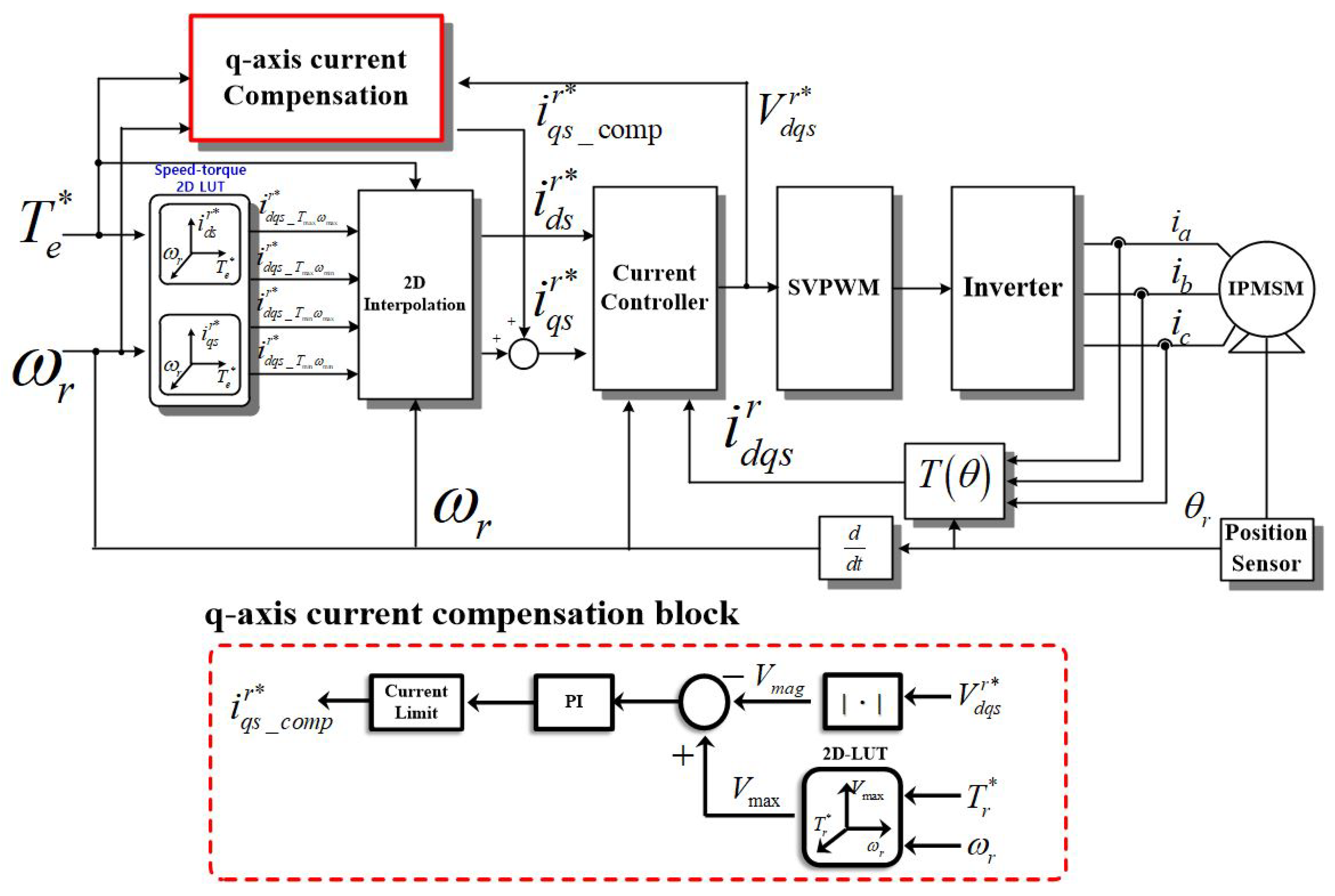
Figure 3 shows a conventional 2D-Interpolation compensation block diagram for the conventional method [
17]. A PI controller is used for interpolation error compensation based on q-axis current in order to reduce the data points of LUT. As shown in the q-axis current compensation block diagram in
Figure 3, if the PI controller is used for compensation based on the voltage error, the compensation error cannot be zero because the compensation references will be ellipsoidal due to the voltage limit ellipse of IPMSM.
Furthermore, although the total memory used for current references can be diminished, a back-Electromotive force(EMF) voltage LUT is required for the conventional compensation method. Moreover, the compensated q-axis current variation is a nonlinear characteristic based on the d-axis current variation, as shown in
Figure 2b, using a PI controller to compensate the current generation is unsuitable because of the time-delayed response. Therefore, the conventional compensation method provides limited improvements in response and memory usage.
3. Proposed q-Axis Current Control for Maximum Power Control of Look-Up Table-Based PMSM Control Method
3.1. Overall Concept of Max Power Control Method
As shown in
Figure 2a, the interpolation error hardly exists in the constant-torque operation region. Therefore, without an interpolated error compensation block under a constant torque operation region, the diminished generation power is insignificant.
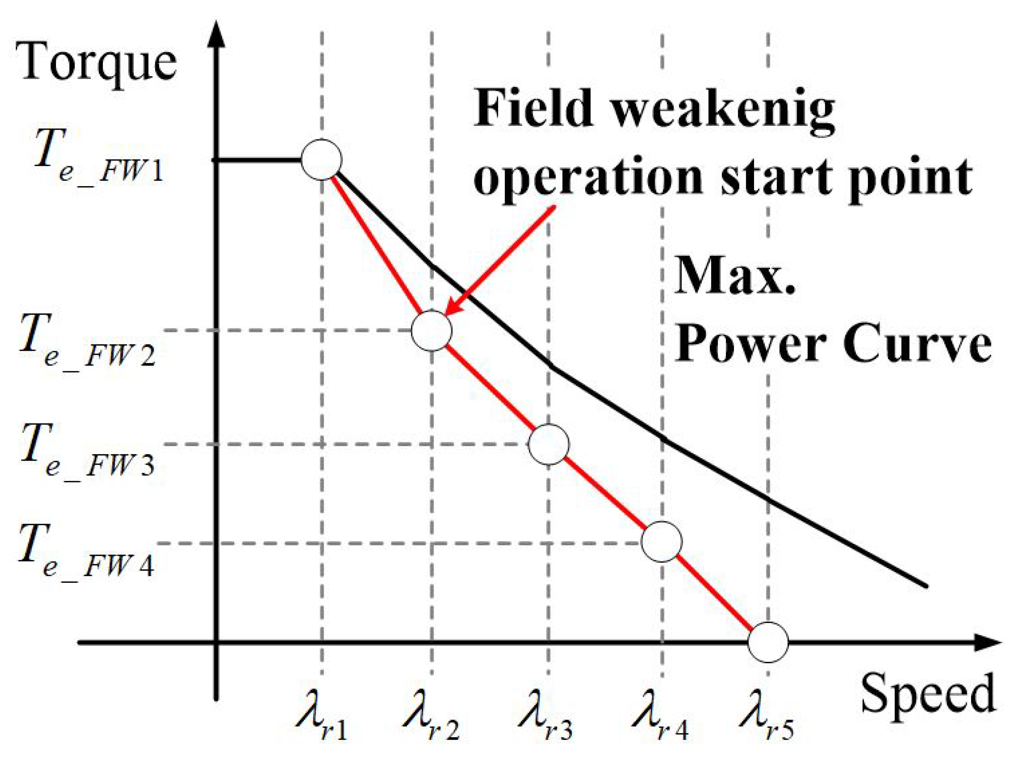
To reduce the stored memory for voltage magnitude, field weakening operation start points of each speed are obtained experimentally instead of voltage magnitudes being obtained throughout the operation region.
Figure 4 shows the stored data of the field weakening starting points. As shown in the figure, as the speed increases, the generated torque reduces to a constant power generation. Additionally, the error between the practical torque–speed curve and interpolated curve hardly exists; based on
Figure 4, the composed control block that determines enable or disable compensation block is shown in
Figure 5. Instead of using speed input, the estimated flux is used to reflect the input voltage variation and reduce the effect of the interpolated error by speed. The conversion method from speed to flux is defined using Equation (
6).
Subsequently, the activated condition of q-axis current compensation can be determined as:
Based on Equation (
7), the input of the compensation controller can be used with the same input as the voltage feedback controller, which is generally used in the flux-torque 2D-LUT-based PMSM control method [
8]. Therefore, it can be defined as Equation (
8):
In contrast, two feedforward controllers are added to the previous compensation method. As mentioned previously, the q-axis current variation in the field-weakening region exhibits a nonlinear characteristic based on the torque variation. Consequently, one feedforward controller is located for the q-axis current regulation and the other for the q-axis current reference compensator. A detailed illustration is provided in the next chapter.
3.2. Feedforward Control Method for q-Axis Current Reference Generator
The proposed feedforward controller for q-axis current compensation is composed of voltage feedforward (Feedforward1) and current feedforward (Feedforward2) control methods. First, voltage feedforward control is based on voltage error Equation (
8). As shown in
Figure 6, the d-axis current reference stored in the LUT generates a proper current for the voltage restriction ellipse. Therefore, if the d-axis current is well-regulated, an insufficient voltage error is caused only by the q-axis current. Thus, the voltage error can be modified as:
where and
are the linear interpolated d-axis and q-axis currents, respectively.
Using Equation (
9), the compensation feedforward current can be easily obtained using Equation (
10).
This compensated q-axis current reference value should always be positive; therefore, it has to respond only to a positive voltage error.
However, the derivative of the q-axis current based on the d-axis current variation from Equation (
4) can be expressed as:
Discretizing Equation (
12) to discretize results in Equation (
13):
When Equation (
13) is modified for the estimated next sample q-axis current, it can be described as below, assuming that the back-EMF voltage is equal to the voltage references.
To implement Equation (
15) in the current reference generator, substitute the practical currents with current references, which is finally modified as Equation (
16).
Equation (
16) indicates that if we know the proper d-axis current reference variation, the q-axis current reference can be deduced from this variation.
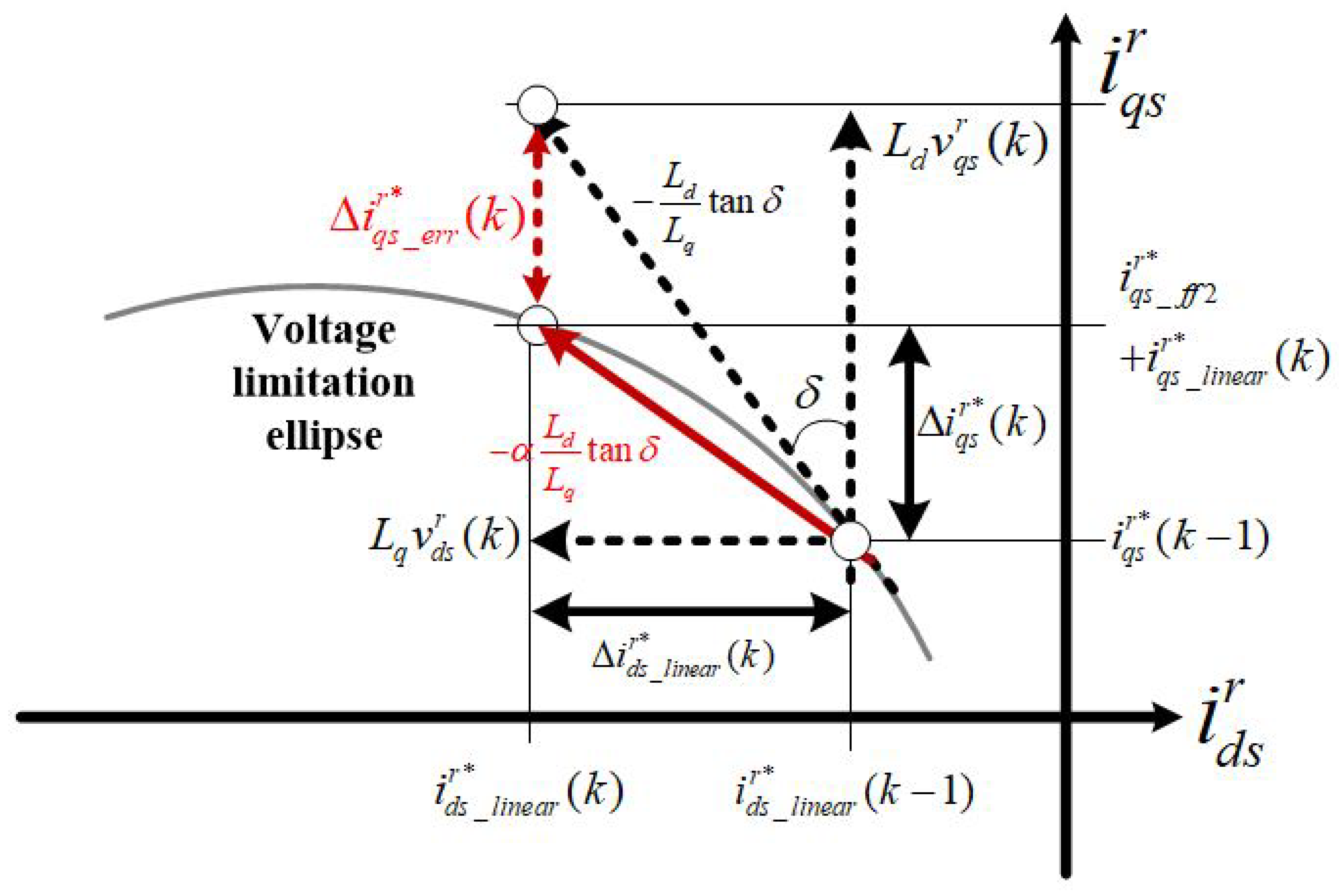
Figure 6 shows the q-axis current variation as per the d-axis current variation. The ratio of dq-axis voltage reference indicates the tangential component of back-EMF direction vector in dq-axis current domain; therefore, with this direction vector, a suitable q-axis current reference for voltage limitation ellipse can be obtained. However, as shown in the figure, there is a quantization error
between the proper and deducted q-axis current reference values. If the control period is not sufficient to ignore this error, a suitable gain that varies with
must be adopted to this gradient.
where
.
Consequently, another feedforward current reference can be obtained as below.
Among the feedforward q-axis compensation currents, the final chosen feedforward is the smaller value. Obviously, an error exists in the feedforward value because of incorrect motor parameters, which can be regulated by the feedback PI controller based on the back-EMF voltage magnitude.
The update period of the current reference should be much slower than that of the current regulation cycle. Moreover, to obtain the effective voltage references regarding the back-EMF, current regulation must be completed until the next current reference update. Additionally, the tangential component of the back-EMF voltage direction vector has to be properly limited, which means that although the d-axis voltage reference is zero, meaning the q-axis current is zero, the calculated q-axis compensation current reference has to be properly limited by the method that avoids zero division.
3.3. Membership Function for Feedforward Controllers
Two feedforward controllers are used for the field weakening current generator. the majorly affected regions are different from each other. As shown in
Figure 5, the low-pass filter is selected to reduce the voltage ripple. Because of this low-pass filter, a delay exists, and a small voltage error cannot be easily detected.
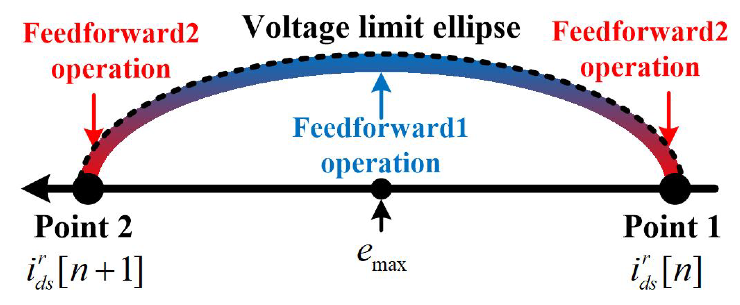
Figure 7 shows how to choose the effective feedforward controller during the field weakening operation region. Feedforward controller 1(FF1), as described in
Figure 5, requires a sufficient voltage error for effective feedforward operation. However, if the motor is operating at the flux/torque point stored in the LUT, this voltage error is very small for feedforward control with FF1. Therefore, the most effective region to compensate for FF1 is the middle range between points 1 and 2, as shown in
Figure 7. Conversely, the feedforward controller 2 (FF2) described in
Figure 5 can effectively compensate for the current when the voltage error hardly exists because the compensation current is determined by the tangential component of the dq-axis voltages.
Because the compensation current only affects the q-axis current, the operation range of FF1 and FF2 is determined by the points of the d-axis currents stored in the LUT, as shown in
Figure 7. The interpolation error (
) is maximized in the middle of the stored operating conditions, which can be described by the d-axis current as Equation (
19).
To classify the operation region using Equation (
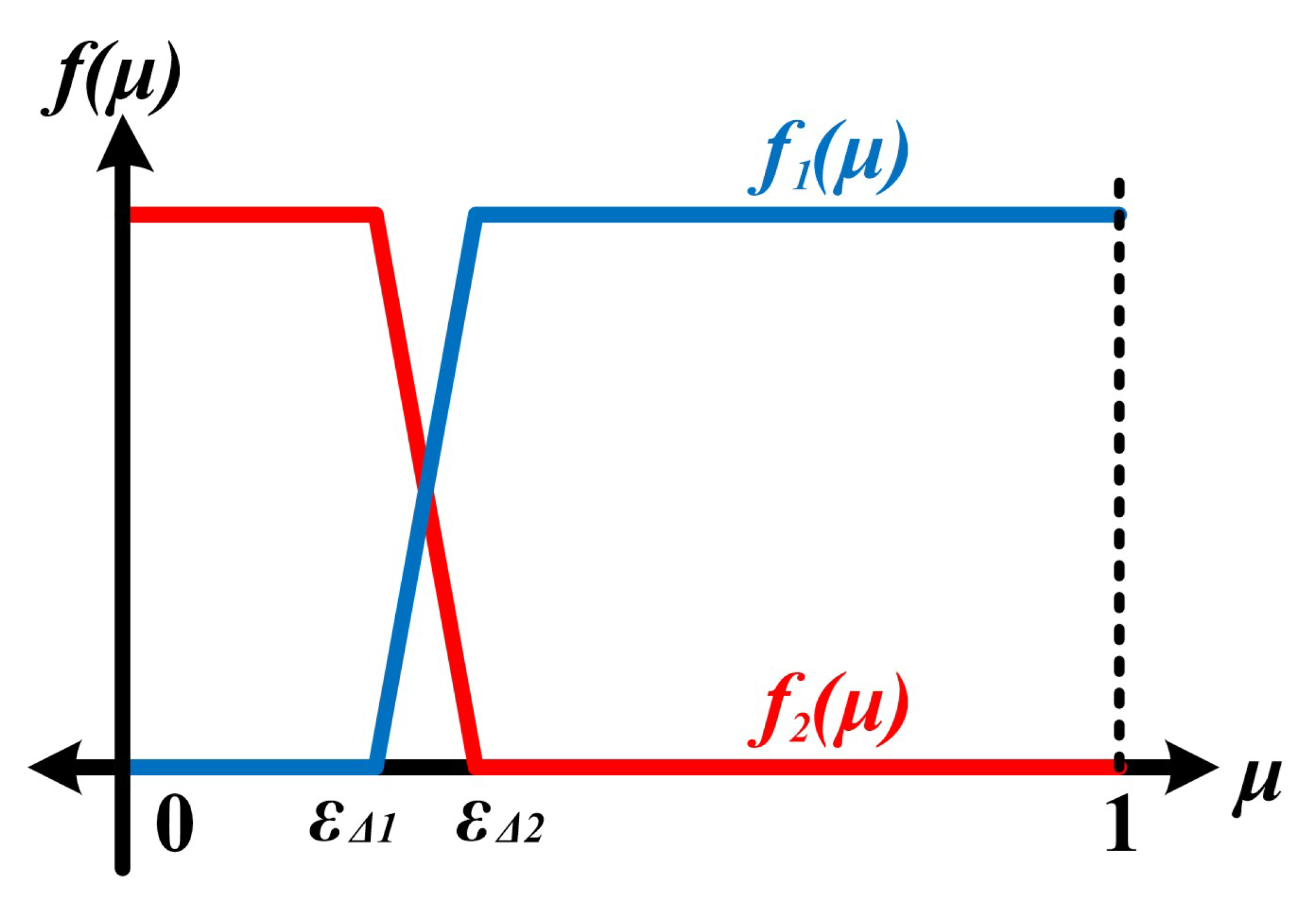
19), the input of the membership function
can be calculated using Equation (
20), and the membership function for choosing the effective feedforward controller is shown in
Figure 8.
As shown in the figure, this membership function operates the feedforward q-axis current reference as in
Figure 7. Note that if
is zero or one, FF2 is selected instead of FF1. Consequently, a suitable transition of the feedforward q-axis current reference can be obtained using Equation (
21).
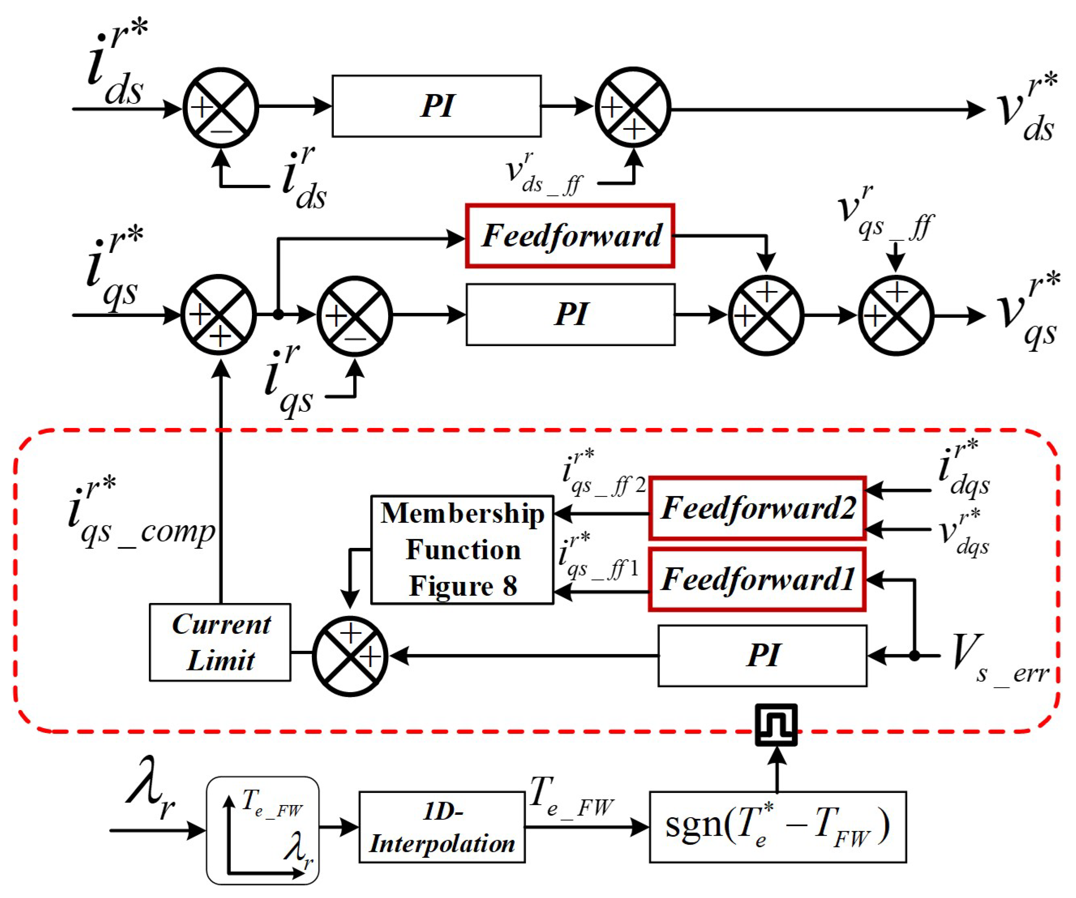
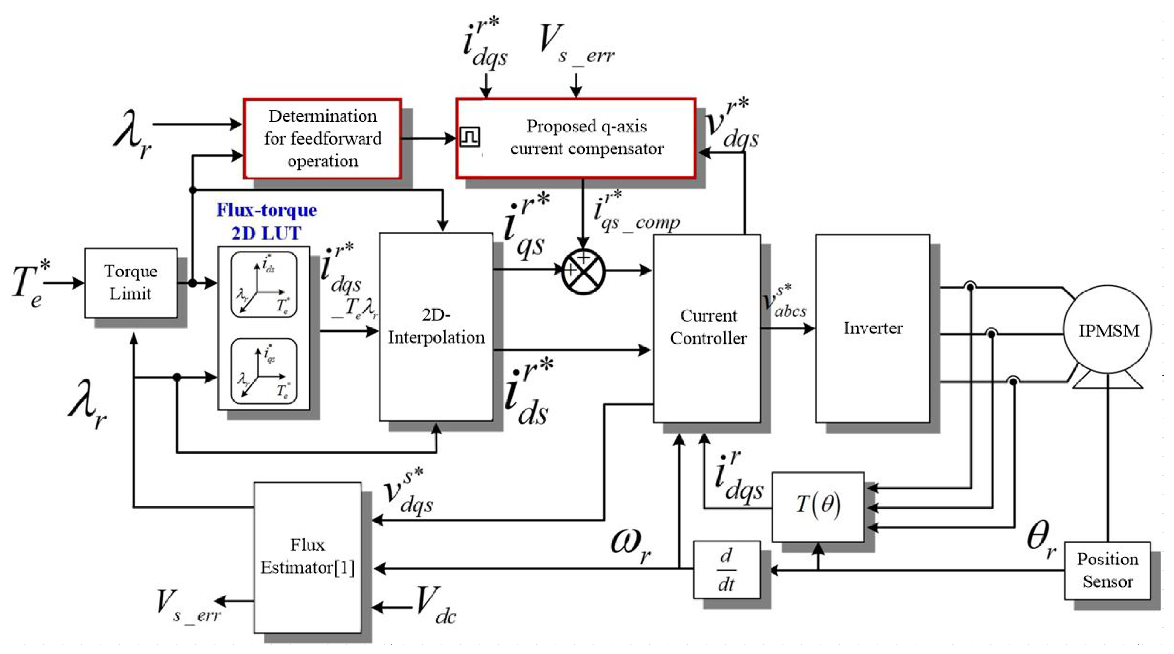
Figure 9 shows the overall proposed LUT-based PMSM control method. In contrast to
Figure 3, the proposed control method comprises a flux-torque 2D-LUT, a determination block in which q-axis current compensation is needed, and a novel q-axis feedforward compensator. In this study,
was selected as 0.25, and
was set to 0.35.
3.4. Experiment Result
The experimental setup comprises the target motor, the IPMSM inverter that enables the interior PMSM (IPMSM) to have a constant speed, and the power electronics drive system.
Figure 10 shows the diagram of the experimental setup, where the speed of the load motor is controlled by the load motor inverter, and the IPMSM is controlled by the IPMSM inverter. The DC-link capacitor is shared in both systems, and an AC/DC PWM converter is also used to maintain the DC-link voltage.
The rated power of the IPMSM is 15 kW, the rated speed is 3400 rpm, and the rated torque is 38 Nm.
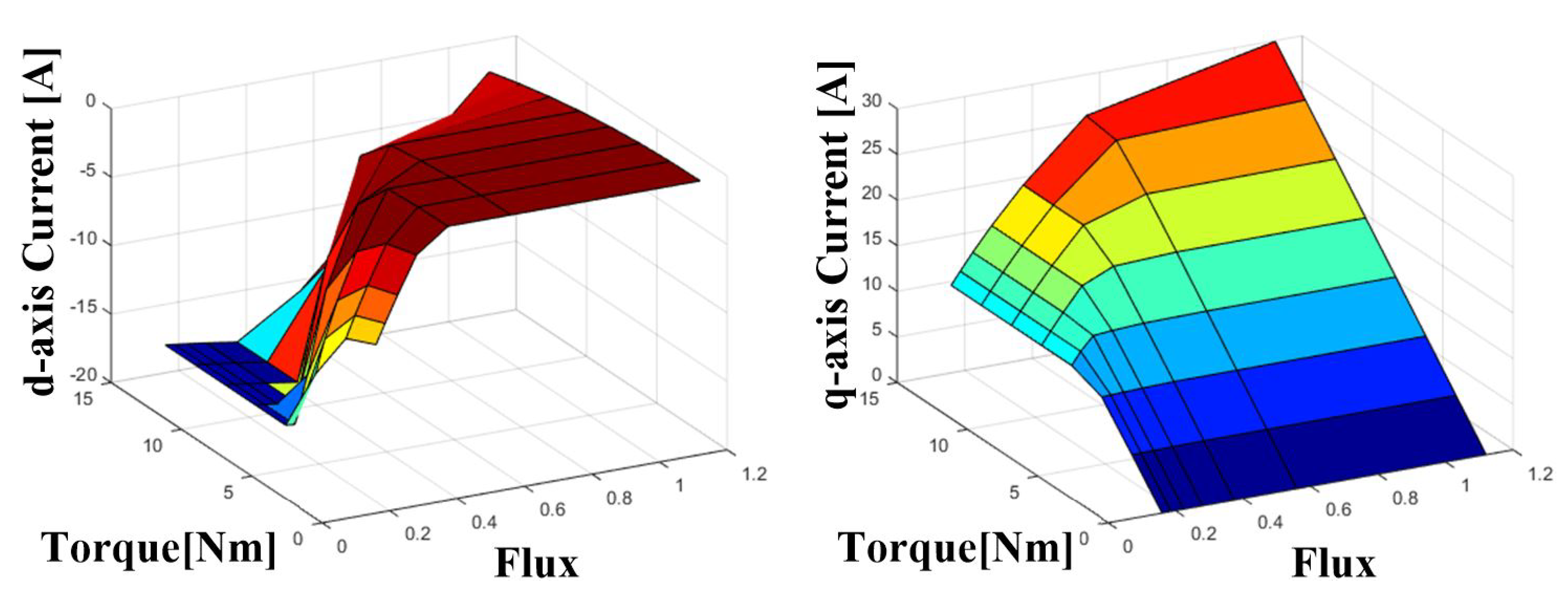
Table 1 lists the parameters of the motor used in the experiment. Although this IPMSM for the experiment might not be suitable for general automotive applications in terms of power and torque, the validity of the proposed method can be proven by it since it shares the same machine characteristics. The d-axis and q-axis current maps for the Maximum Torque per Ampere (MTPA) control for the IPMSM, based on the motor speed and torque, were made through experiments, as shown in
Figure 11. For more challenging experimental conditions, the data storage for the current map was minimized. In this study, the current map data for the experiments were stored by one-fourth of the maximum torque, which only has the current data for two torque points except for the current data for the maximum and zero torque control. The output power is lower than the known parameter of the actual motor because the parameter becomes incorrect owing to the experimental conditions, such as the saturation effect.
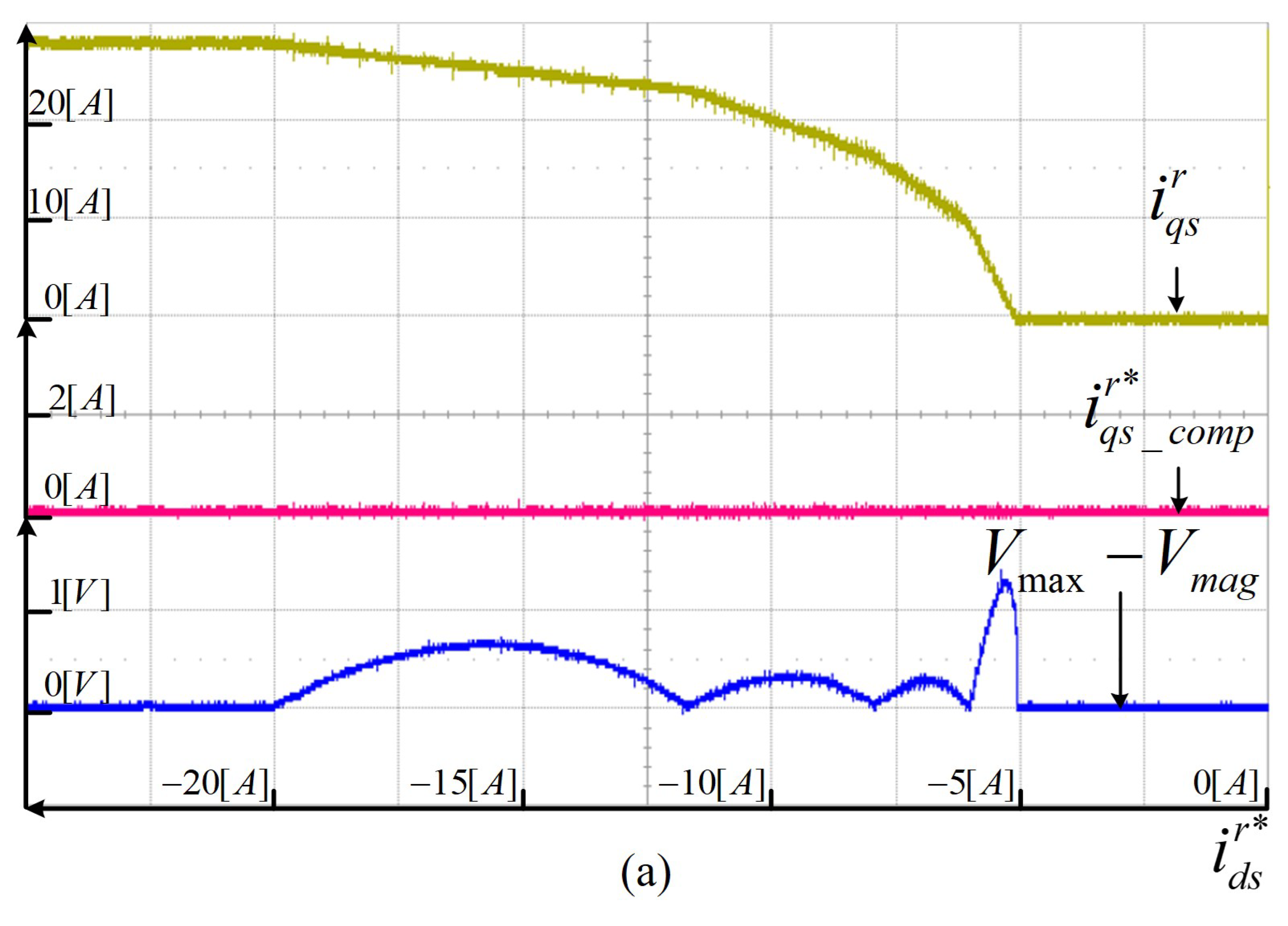
Figure 12a shows the field weakening operation experiment when only the 2D-Interpolation is adapted [
10,
11].
is linearly compensated based on the current data for the field weakening operation, and the error between
and
shows the error between the voltage limit ellipse and back-EMF. This means the output power is lower than the maximum output power available for the corresponding speed in the conventional method.
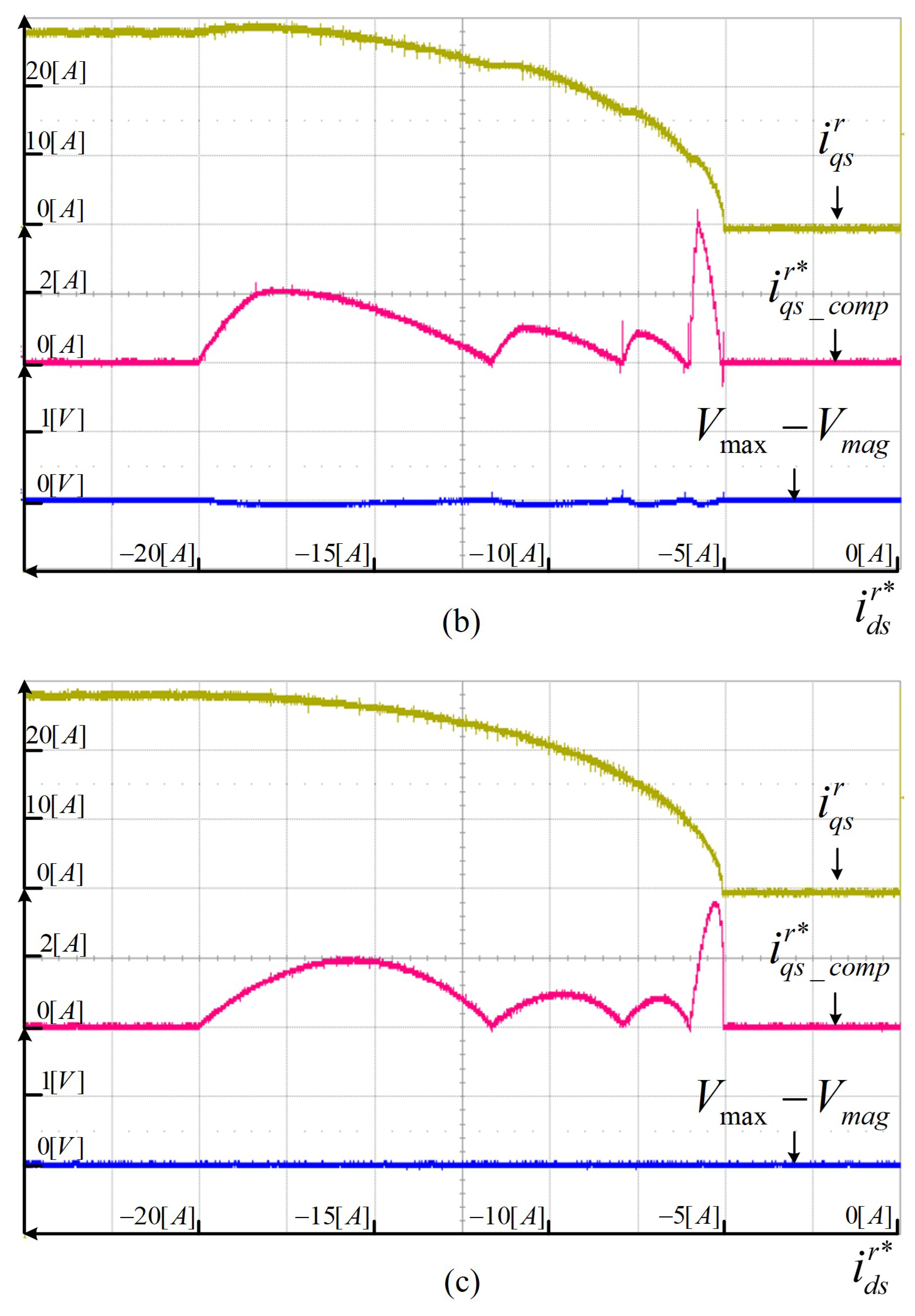
Figure 12b shows the waveform of the experimental result when the q-axis current is compensated using Feedforward1 and the PI controller under the same conditions as in
Figure 12a [
17,
18]. As shown in the waveform of the experimental result,
increases with
, which is the q-axis current, increasing owing to
. There is a moment when
becomes larger than
; however, this phenomenon results from reflecting the characteristics of the PI controller. Consequently, the error between the voltage limit ellipse and back-emf voltage, represented by the error between
and
, is reduced; nonetheless, some negative error remains because of the aforementioned delay from the low-pass filter.
Figure 12c shows the experimental results when the proposed “PI controller” and “Feedforward1” and “Feedforward2” feedforward compensators are adapted. As indicated by the
waveform in
Figure 12c, the dq-axis current locus draws an ellipse instead of a straight line, unlike the
in
Figure 12a, to which the conventional method is applied. The reasons are as follows. As shown by the
waveform, the q-axis current reference was compensated by the proposed q-axis current compensator, as shown by the
waveform. From the
waveform, the error between
and
is reduced in the field weakening region through the increase in the q-axis current compared to the conventional method. Therefore, the proposed method can achieve maximum power control even if there are no current data generated offline.
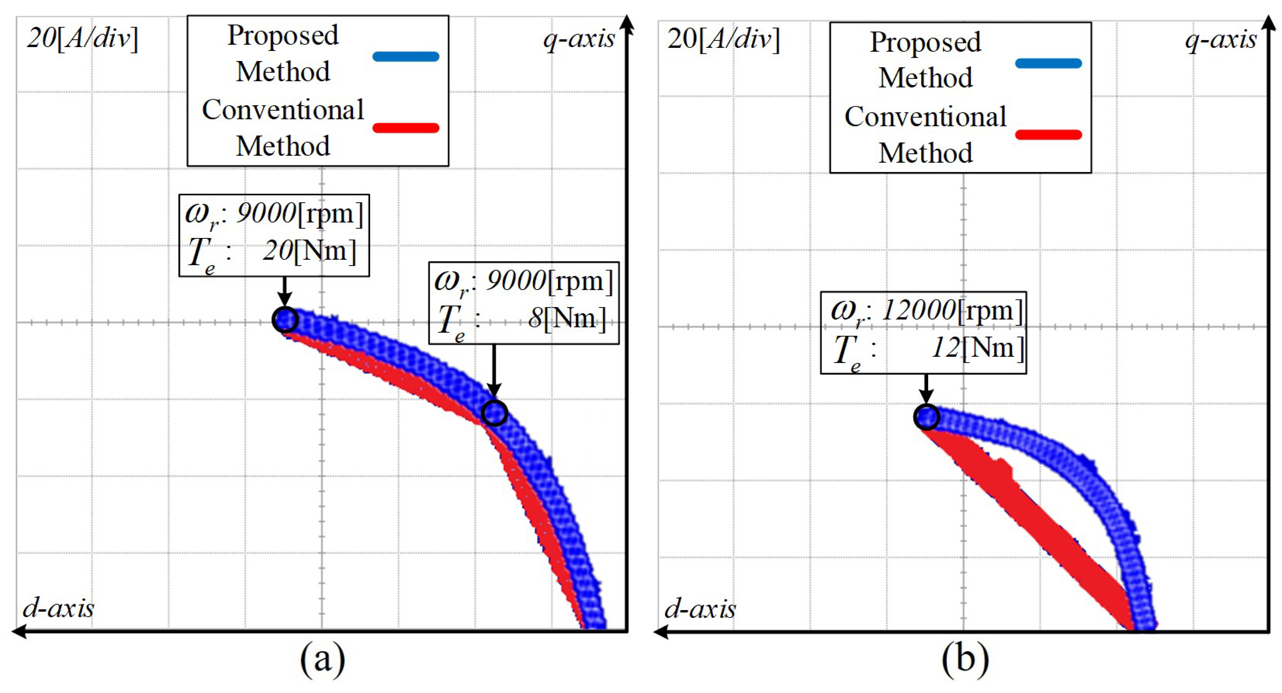
Figure 13 shows a comparison of the experimental results of the conventional compensation method using 2D interpolation and the proposed compensation method. As shown in the figure, the proposed method outputs more power than the conventional method. As can be seen in
Figure 13, there are three-point LUT data at 9000 rpm and two at 12,000 rpm. Therefore, it can be confirmed that the difference in
Figure 13b is larger than the difference between the proposed method and the conventional method in
Figure 13a. Consequently, the smaller the number of look-up table data, the better the performance of the proposed method.


