
How Much Can Small-Scale Wind Energy Production Contribute to Energy Supply in Cities? A Case Study of Berlin


Abstract
:1. Introduction
- 1.
- How much energy could be produced in Berlin through the installation of roof-mounted turbines?
- 2.
- By how much could CO2 emissions be reduced in Berlin?
- 3.
- By how much would the installation of a single roof-mounted SWT result in a profit or loss in Berlin?
2. Methods
2.1. Derivation of Wind Energy Potential
2.2. Economic Evaluation
3. Study Region and Data
3.1. Study Region Berlin
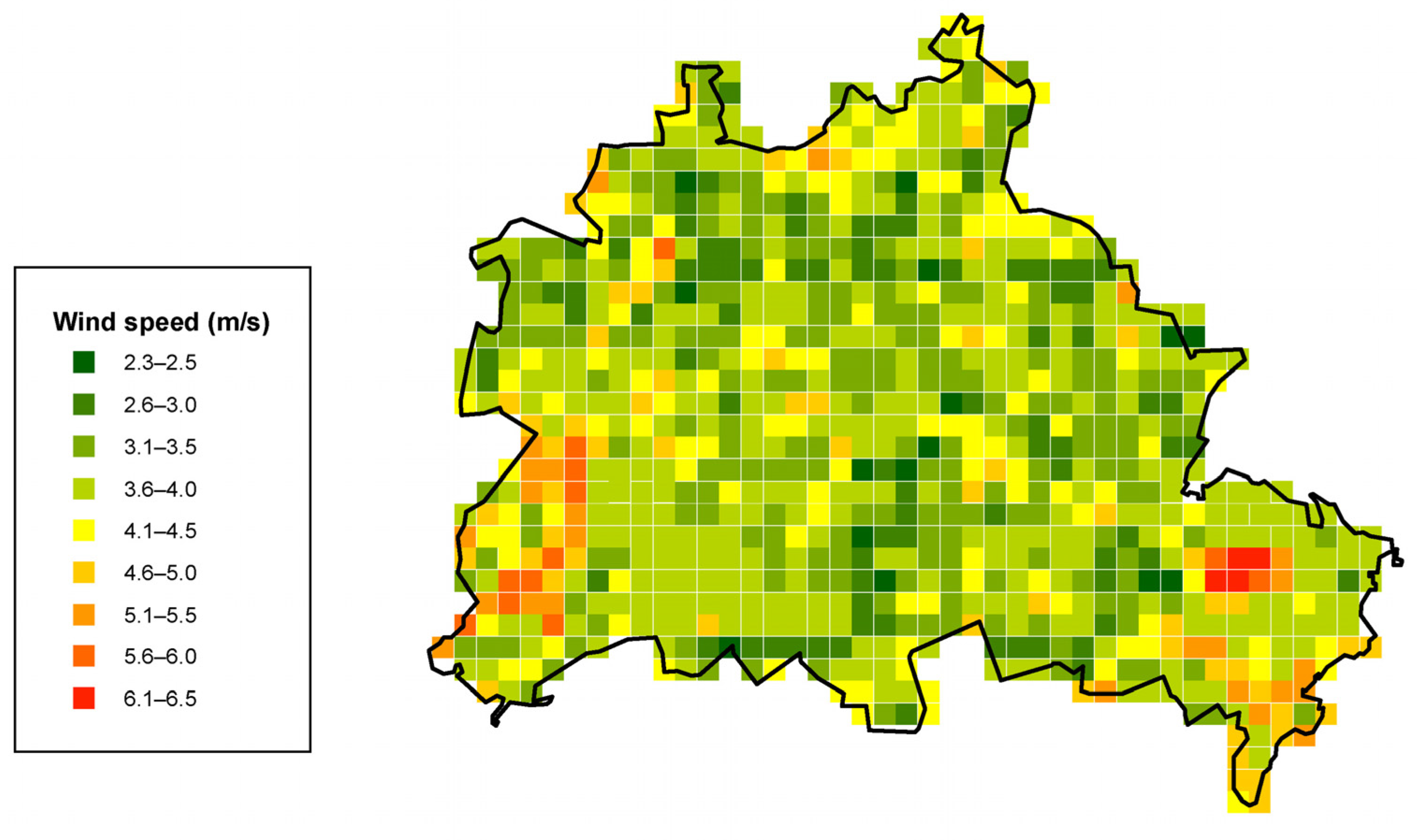
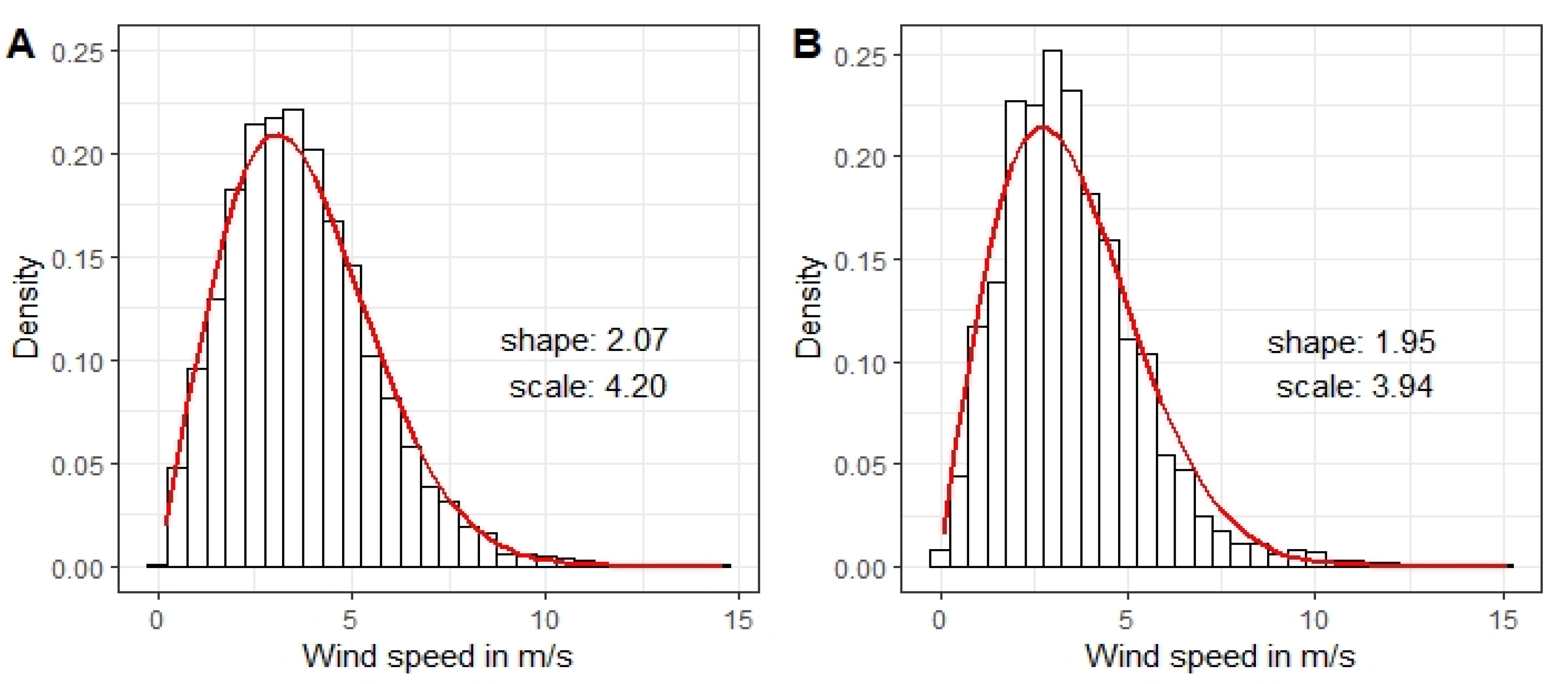
3.2. Wind Data
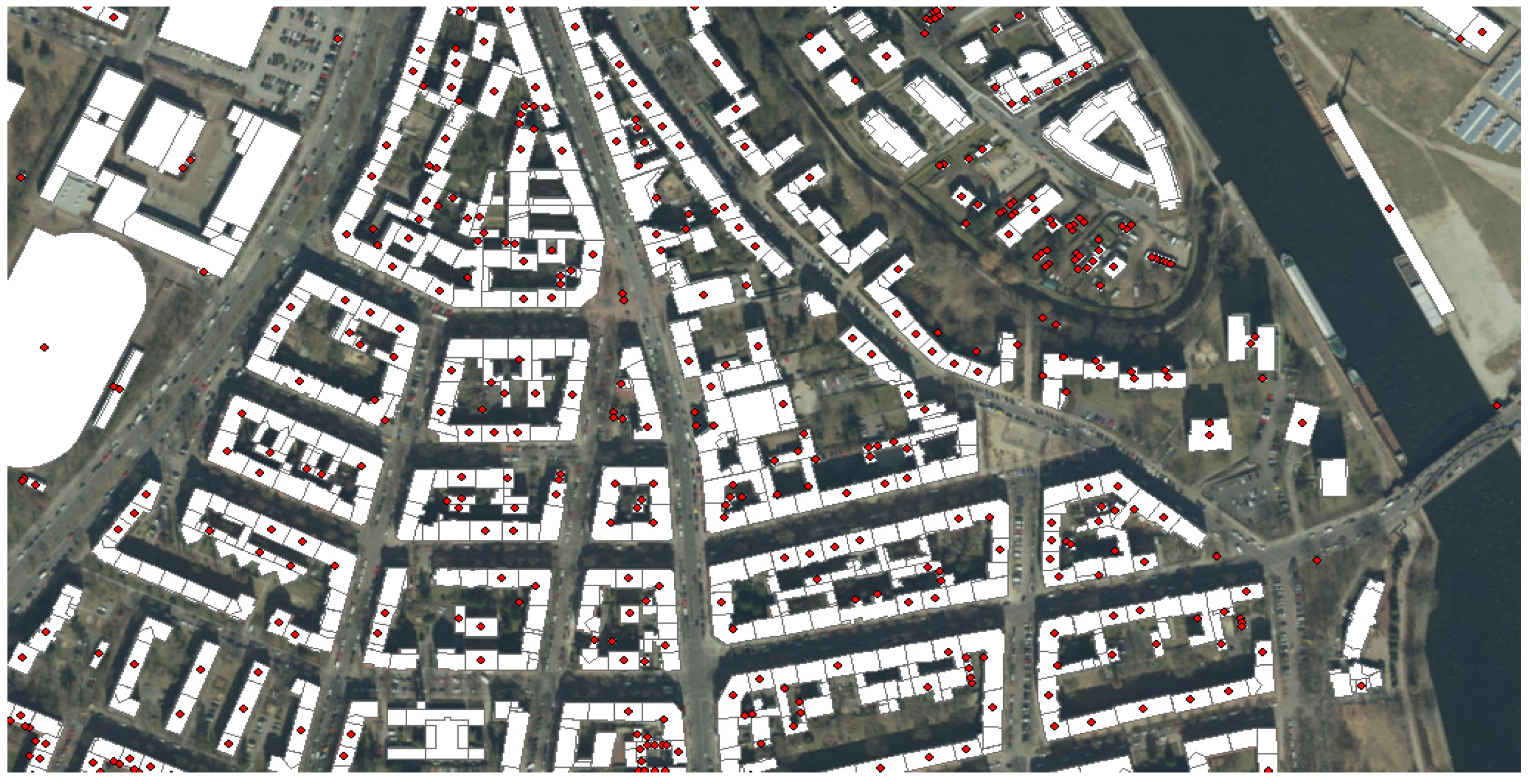
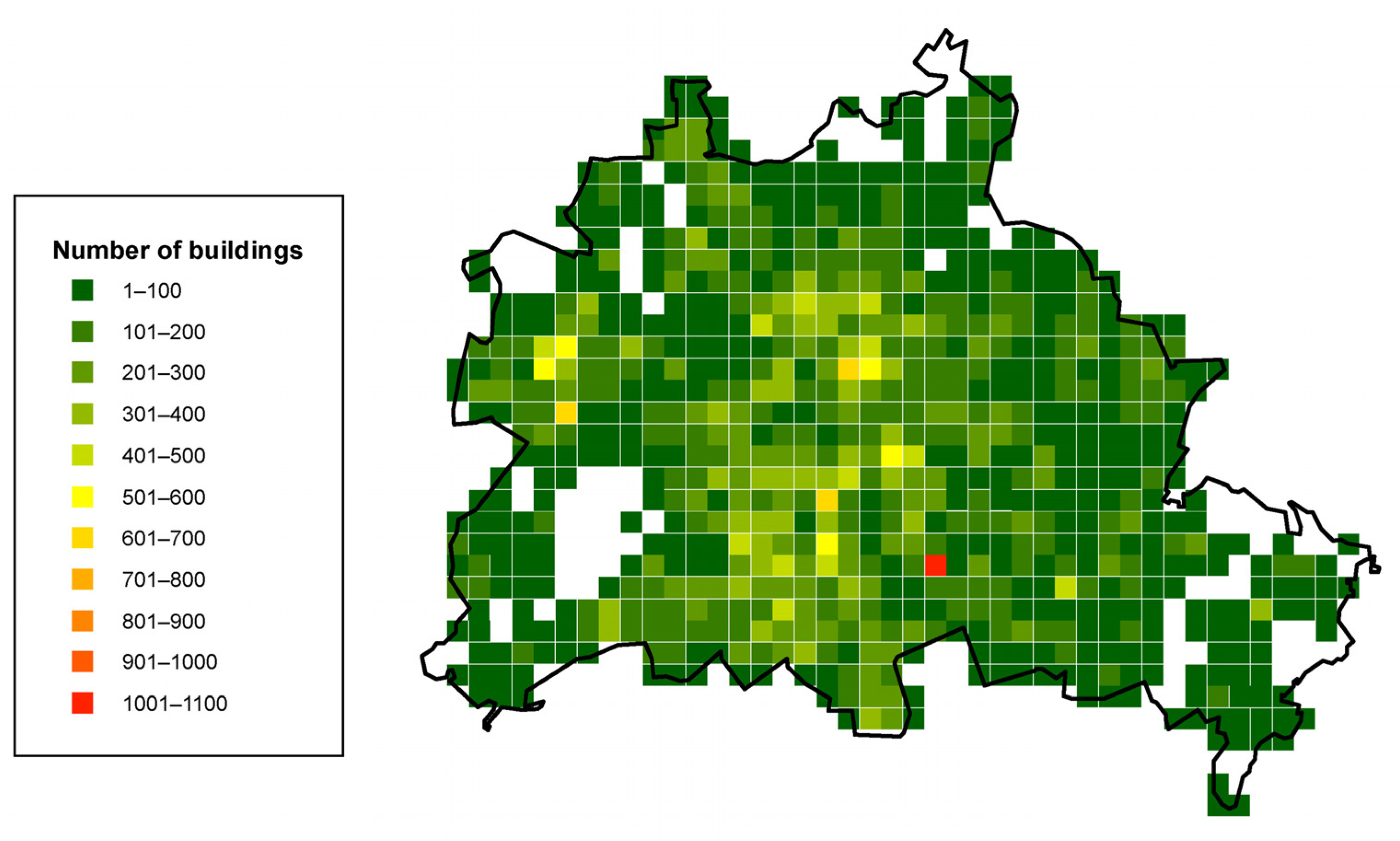
3.3. Building Data
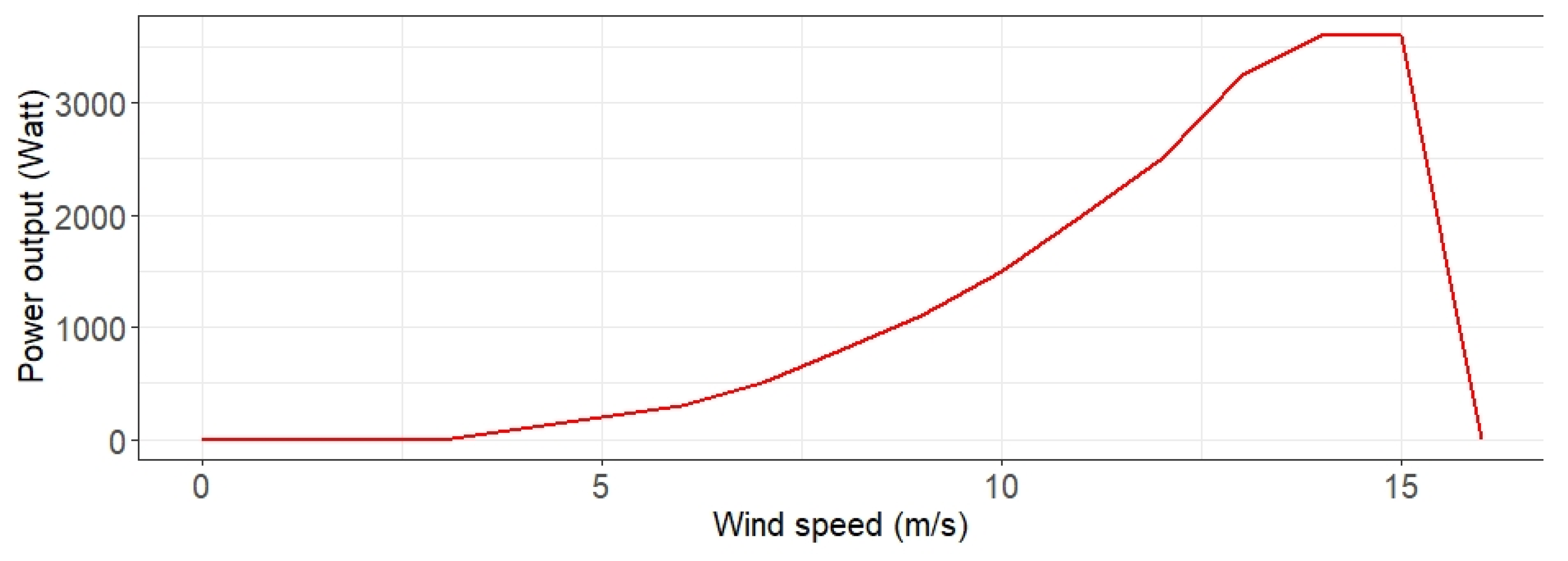
3.4. Reference Turbine
4. Results
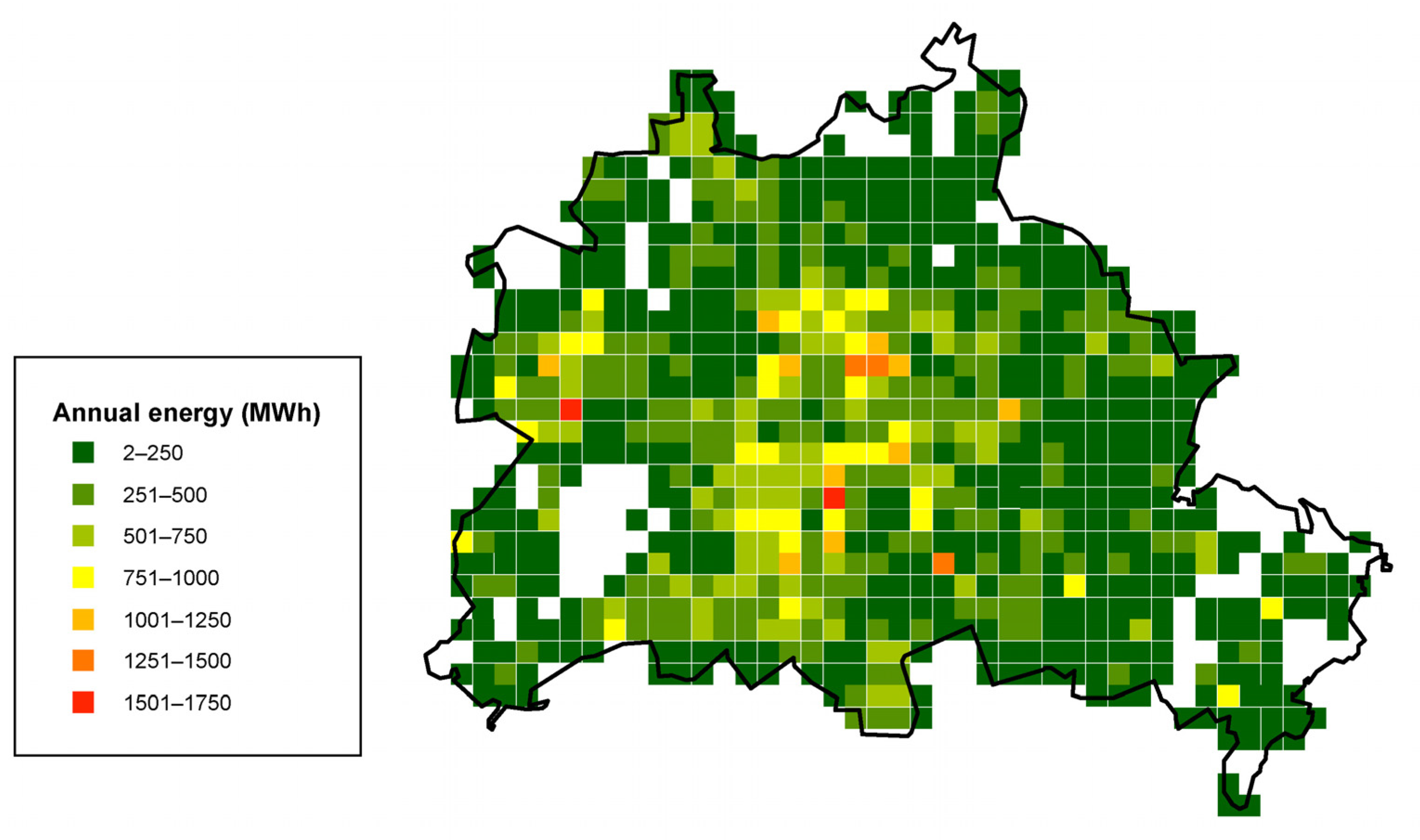
4.1. City-Level
4.1.1. Scenarios—Varying the Number of Turbines per Building
4.1.2. Sensitivity Analysis
4.2. Household-Level
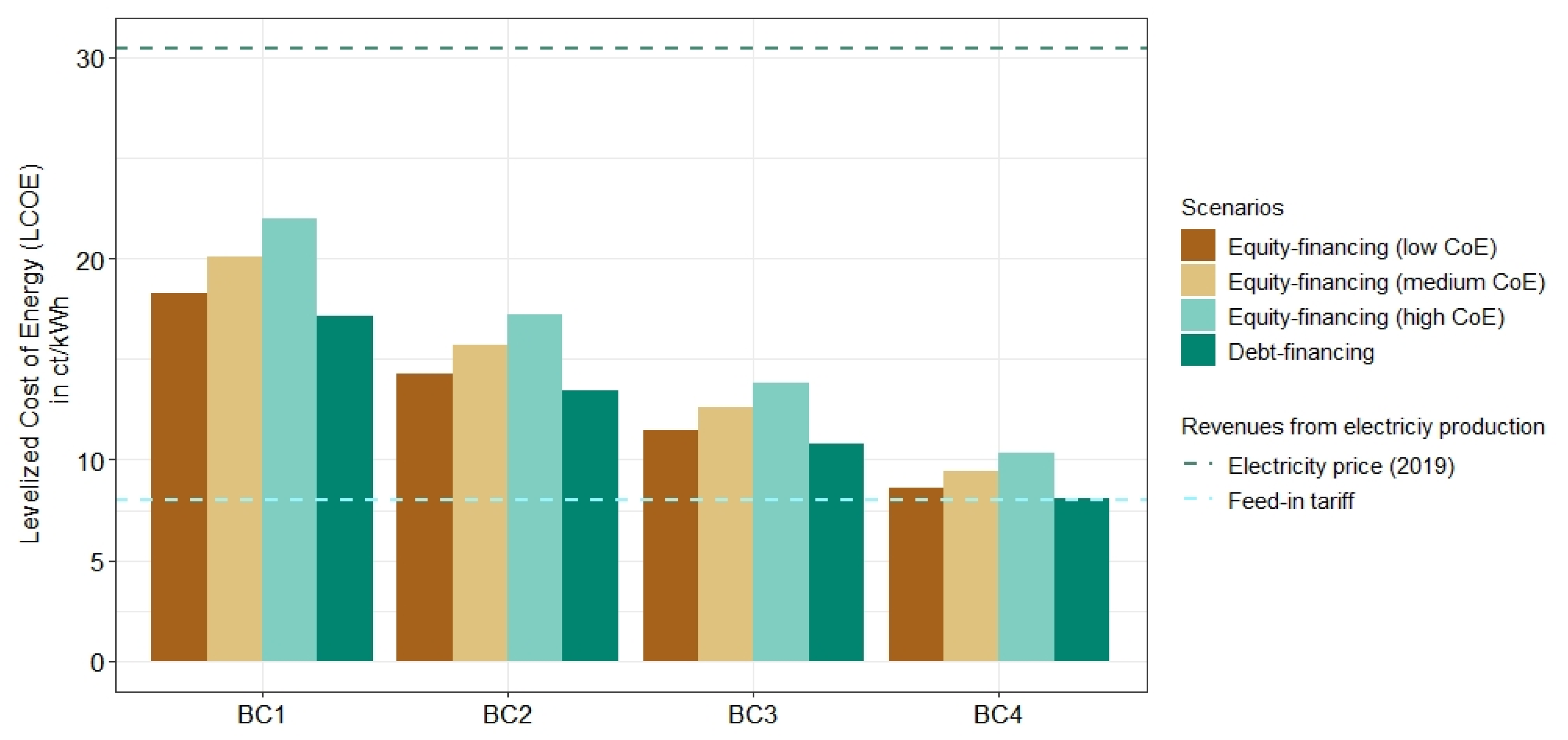
4.3. Economic Evaluation
5. Discussion
6. Conclusions
Author Contributions
Funding
Data Availability Statement
Conflicts of Interest
Appendix A. Building Dataset—Transformation Process
Appendix B. Economic Evaluation
- The produced energy is sold to the grid provider:
- 2.
- The produced energy is self-consumed:
References
- International Energy Agency. Global Energy Review 2021. Assessing the Effects of Economic Recoveries on Global Energy Demand and CO2 Emissions in 2021. Available online: https://www.iea.org/reports/global-energy-review-2021/renewables (accessed on 18 February 2021).
- International Energy Agency. World Energy Balances: Overview. Available online: https://www.iea.org/reports/world-energy-balances-overview/world (accessed on 18 August 2021).
- Busu, M.; Nedelcu, A.C. Analyzing the renewable energy and CO2 emission levels nexus at an EU level: A panel data regression approach. Processes 2021, 9, 130. [Google Scholar] [CrossRef]
- Azam, A.; Rafiq, M.; Shafique, M.; Zhang, H.; Yuan, J. Analyzing the effect of natural gas, nuclear energy and renewable energy on GDP and carbon emissions: A multi-variate panel data analysis. Energy 2021, 219, 119592. [Google Scholar] [CrossRef]
- United Nations. The Paris Agreement. 2015. Available online: http://unfccc.int/files/essential_background/convention/application/pdf/english_paris_agreement.pdf (accessed on 15 July 2021).
- European Commission. Delivering the European Green Deal. Available online: https://ec.europa.eu/info/strategy/priorities-2019–2024/european-green-deal/delivering-european-green-deal_en (accessed on 22 August 2021).
- Baltagi, B.H.; Bresson, G.; Etienne, J.-M. Carbon dioxide emissions and economic activities: A mean field variational bayes semiparametric panel data model with random coefficients. Ann. Econ. Stat. 2019, 134, 43–77. [Google Scholar] [CrossRef]
- Hyams, M.A. Wind energy in the built environment. In Metropolitan Sustainability: Understanding and Improving the Urban Environment; Zeman, F., Ed.; Woodhead Pub. Ltd.: Cambridge, UK, 2012; pp. 457–499. ISBN 9780857090461. [Google Scholar]
- Scholten, D.; Criekemans, D.; van de Graaf, T. An energy transition amidst great power rivalry. J. Int. Aff. 2019, 73, 195–204. [Google Scholar]
- Grieser, B.; Sunak, Y.; Madlener, R. Economics of small wind turbines in urban settings: An empirical investigation for Germany. Renew. Energy 2015, 78, 334–350. [Google Scholar] [CrossRef]
- Bortolini, M.; Gamberi, M.; Graziani, A.; Manzini, R.; Pilati, F. Performance and viability analysis of small wind turbines in the European Union. Renew. Energy 2014, 62, 629–639. [Google Scholar] [CrossRef]
- KC, A.; Whale, J.; Urmee, T. Urban wind conditions and small wind turbines in the built environment: A review. Renew. Energy 2019, 131, 268–283. [Google Scholar] [CrossRef]
- V, Sri Ragunath and Pandey, Jitendra K and Mondal, Amit Kumar and Karn, Ashish, Electricity Generation from Wind Turbines at Low Wind Velocities: A Review. 2019. Available online: https://ssrn.com/abstract=3372736 (accessed on 31 August 2021).
- Chong, W.T.; Pan, K.C.; Poh, S.C.; Fazlizan, A.; Oon, C.S.; Badarudin, A.; Nik-Ghazali, N. Performance investigation of a power augmented vertical axis wind turbine for urban high-rise application. Renew. Energy 2013, 51, 388–397. [Google Scholar] [CrossRef]
- Wen, W.T.; Palanichamy, C.; Ramasamy, G. Small wind turbines as partial solution for energy sustainability in Malaysia. Int. J. Energy Econ. Policy 2019, 9, 257–266. [Google Scholar]
- Arteaga-López, E.; Angeles-Camacho, C. Innovative virtual computational domain based on wind rose diagrams for micrositing small wind turbines. Energy 2020, 220, 119701. [Google Scholar] [CrossRef]
- Ishugah, T.; Li, Y.; Wang, R.; Kiplagat, J. Advances in wind energy resource exploitation in urban environment: A review. Renew. Sustain. Energy Rev. 2014, 37, 613–626. [Google Scholar] [CrossRef]
- Twele, J. Empfehlungen zum Einsatz kleiner Windenergieanlagen im urbanen Raum; Reiner Lemoine Institute: Berlin, Germany, 2015. [Google Scholar]
- Stathopoulos, T.; Alrawashdeh, H.; Al-Quraan, A.; Blocken, B.; Dilimulati, A.; Parashivoiu, M.; Pilay, P. Urban wind energy: Some views on potential and challenges. J. Wind Eng. Ind. Aerodyn. 2018, 179, 146–157. [Google Scholar] [CrossRef]
- Battisti, L.; Benini, E.; Brighenti, A.; Dell’Anna, S.; Castelli, M.R. Small wind turbine effectiveness in the urban environment. Renew. Energy 2018, 129, 102–113. [Google Scholar] [CrossRef]
- Hupfer, P.; Chmielewski, F.-M. (Eds.) Das Klima von Berlin; Akademie-Verlag: Berlin, Germany, 1990; ISBN 3055006305. [Google Scholar]
- Hupfer, P.; Becker, P.; Börngen, M. 20,000 Jahre Berliner Luft: Klimaschwankungen im Berliner Raum; Gutenbergplatz: Leipzig, Germany, 2013; ISBN 9783937219622. [Google Scholar]
- Gualtieri, G.; Secci, S. Methods to extrapolate wind resource to the turbine hub height based on power law: A 1-h wind speed vs. Weibull distribution extrapolation comparison. Renew. Energy 2012, 43, 183–200. [Google Scholar] [CrossRef]
- Gualtieri, G.; Secci, S. Comparing methods to calculate atmospheric stability-dependent wind speed profiles: A case study on coastal location. Renew. Energy 2011, 36, 2189–2204. [Google Scholar] [CrossRef]
- Counihan, J. Adiabatic atmospheric boundary layers: A review and analysis of data from the period 1880–1972. Atmos. Environ. 1975, 9, 871–905. [Google Scholar] [CrossRef]
- Manwell, J.F.; McGowan, J.G.; Rogers, A.L. Wind Energy Explained; John Wiley & Sons, Ltd.: Chichester, UK, 2009; ISBN 9781119994367. [Google Scholar]
- Elnaggar, M.; Edwan, E.; Ritter, M. Wind energy potential of Gaza using small wind turbines: A feasibility study. Energies 2017, 10, 1229. [Google Scholar] [CrossRef]
- Irwin, J.S. A theoretical variation of the wind profile power-law exponent as a function of surface roughness and stability. Atmos. Environ. 1979, 13, 191–194. [Google Scholar] [CrossRef]
- Cleveland, C.J.; Morris, C.G. Dictionary of Energy, 2nd ed.; Elsevier: Amsterdam, The Netherlands, 2015; ISBN 0080968120. [Google Scholar]
- Smedman-Högström, A.-S.; Höström, U. A practical method for determining wind frequency distributions for the lowest 200 m from routine meteorological data. J. Appl. Meteorol. 1978, 17, 942–954. [Google Scholar] [CrossRef]
- WMO. Guide to Meteorological Instruments and Methods of Observation; (WMO-No. 8); WMO: Geneva, Switzerland, 2018; ISBN 978-92-63-10008-5. [Google Scholar]
- Sunderland, K.M.; Narayana, M.; Putrus, G.; Conlon, M.F.; McDonald, S. The cost of energy associated with micro wind generation: International case studies of rural and urban installations. Energy 2016, 109, 818–829. [Google Scholar] [CrossRef]
- Egli, F.; Steffen, B.; Schmidt, T.S. A dynamic analysis of financing conditions for renewable energy technologies. Nat. Energy 2018, 3, 1084–1092. [Google Scholar] [CrossRef]
- Steffen, B. Estimating the cost of capital for renewable energy projects. Energy Econ. 2020, 88, 104783. [Google Scholar] [CrossRef]
- Ragheb, M. Economics of Wind Power Generation; Elsevier: Amsterdam, The Netherlands, 2017; pp. 537–555. [Google Scholar] [CrossRef]
- MWEA. Domestic Roof-Mounted Wind Turbines: The Current State of the Art. 2005. Available online: https://www.solarcollect.co.uk/downloads/domturbinerep.pdf (accessed on 31 August 2021).
- Amt für Statistik Berlin-Brandenburg. Kleine Statistik Berlin 2018; Amt für Statistik Berlin-Brandenburg: Potsdam, Germany, 2018; Available online: https://www.statistik-berlin-brandenburg.de/kleine-statistiken-6bffdf63bfa0f54c (accessed on 31 August 2021).
- BauO Bln. Bauordnung für Berlin. 2011. Available online: http://www.bauordnungen.de/Berlin.pdf (accessed on 31 August 2021).
- Deutscher Wetterdienst (DWD). Bundesamt für Bauwesen und Raumordnung. Testreferenzjahre (TRY). Available online: https://www.dwd.de/DE/leistungen/testreferenzjahre/testreferenzjahre.html (accessed on 15 July 2021).
- Krähenmann, S.; Walter, A.; Brienen, S.; Imbery, F.; Matzarakis, A. High-resolution grids of hourly meteorological variables for Germany. Theor. Appl. Clim. 2016, 131, 899–926. [Google Scholar] [CrossRef] [Green Version]
- Lun, I.Y.; Lam, J.C. A study of Weibull parameters using long-term wind observations. Renew. Energy 2000, 20, 145–153. [Google Scholar] [CrossRef]
- Deutscher Wetterdienst. Hourly Historical Wind Data. Available online: https://opendata.dwd.de/climate_environment/CDC/observations_germany/climate/hourly/wind/ (accessed on 15 July 2021).
- Senatsverwaltung für Stadtentwicklung und Wohnen Berlin. 3D-Gebäudemodelle im Level of Detail 1 (LoD 1) [Atom]. Available online: https://daten.berlin.de/datensaetze/3d-gebäudemodelle-im-level-detail-1-lod-1-atom (accessed on 31 August 2021).
- En-eco. Skyline sl-30, Technial Specifications: 3 kW Vertical Axis Wind Turbine. Available online: https://www.solarenergypoint.it/catalogo/schede_tecniche/eolico/en-eco/en-eco_skyline_3_kw_scheda_tecnica.pdf (accessed on 31 August 2021).
- AfS. Energie- und CO2-Bilanz in Berlin 2017: Statistischer Bericht E IV 4-j/17. 2019. Available online: https://www.statistik-berlin-brandenburg.de/publikationen/stat_berichte/2019/SB_E04-04-00_2017j01_BE.pdf (accessed on 31 August 2021).
- Magnusson, M.; Smedman, A.-S. Air flow behind wind turbines. J. Wind. Eng. Ind. Aerodyn. 1999, 80, 169–189. [Google Scholar] [CrossRef]
- Ritter, M.; Deckert, L. Site assessment, turbine selection, and local feed-in tariffs through the wind energy index. Appl. Energy 2017, 185, 1087–1099. [Google Scholar] [CrossRef]
- Kenny, W.; Corscadden, K.; Lubitz, W.D.; Thomson, A.; McCabe, J. Investigation of wake effects on the energy production of small wind turbines. Wind. Eng. 2013, 37, 151–163. [Google Scholar] [CrossRef]
- Barthelmie, R.J.; Hansen, K.; Frandsen, S.T.; Rathmann, O.; Schepers, J.G.; Schlez, W.; Phillips, J.; Rados, K.; Zervos, A.; Politis, E.S.; et al. Modelling and measuring flow and wind turbine wakes in large wind farms offshore. Wind. Energy 2009, 12, 431–444. [Google Scholar] [CrossRef]
- Rezaeiha, A.; Montazeri, H.; Blocken, B. A framework for preliminary large-scale urban wind energy potential assessment: Roof-mounted wind turbines. Energy Convers. Manag. 2020, 214, 112770. [Google Scholar] [CrossRef]
- EEG. Gesetz für den Vorrang Erneuerbarer Energien (Erneuerbare-Energien-Gesetz—EEG 2000). 2000. Available online: https://www.bgbl.de (accessed on 31 August 2021).
- Kleinwindanlagen. Handbuch der Technik, Genehmigung und Wirtschaftlichkeit Kleiner Windräder; Franken, M., Ed.; Bundesverband Wind Energie: Berlin, Germany, 2013; ISBN 9783942579179. [Google Scholar]
- Jüttemann, P. Wichtige Themen zu Kleinwindkraftanlagen. Available online: https://www.klein-windkraftanlagen.com/ (accessed on 17 February 2020).
- Feddersen, C.; Franken, M.; Jensen, D.; Jüttemann, P.; Lehmkuhl, V.; Rentzing, S.; Weller, K. Energiewende selber machen; Bundesverband Windenergie: Berlin, Germany, 2015; ISBN 978-3942579278. [Google Scholar]
- Pitteloud, J.-D.; Gsänger, S. Small Wind World Report 2017: Summary. 2017. Available online: http://www.wwindea.org/download/SWWR2017-SUMMARY(2).pdf (accessed on 15 July 2021).
- BMWi. EEG-Vergütung und Kapazitätszuweisung. Available online: https://www.erneuerbare-energien.de/EE/Navigation/DE/Technologien/Windenergie-auf-See/Finanzierung/EEG-Verguetung/eeg-verguetung.htm (accessed on 31 August 2021).
- Mamkhezri, J.; Thacher, J.A.; Chermak, J.M. Consumer preferences for solar energy: A choice experiment study. Energy J. 2020, 41. [Google Scholar] [CrossRef]
- Harold, J.; Bertsch, V.; Lawrence, T.; Hall, M. Drivers of people’s preferences for spatial proximity to energy infrastructure technologies: A cross-country analysis. Energy J. 2021, 42. [Google Scholar] [CrossRef]
- Kolb, S.; Dillig, M.; Plankenbühler, T.; Karl, J. The impact of renewables on electricity prices in Germany—An update for the years 2014–2018. Renew. Sustain. Energy Rev. 2020, 134, 110307. [Google Scholar] [CrossRef]
- Cludius, J.; Hermann, H.; Matthes, F.C.; Graichen, V. The merit order effect of wind and photovoltaic electricity generation in Germany 2008–2016: Estimation and distributional implications. Energy Econ. 2014, 44, 302–313. [Google Scholar] [CrossRef]
- Rai, A.; Nunn, O. On the impact of increasing penetration of variable renewables on electricity spot price extremes in Australia. Econ. Anal. Policy 2020, 67, 67–86. [Google Scholar] [CrossRef] [PubMed]
- Dillig, M.; Jung, M.; Karl, J. The impact of renewables on electricity prices in Germany—An estimation based on historic spot prices in the years 2011–2013. Renew. Sustain. Energy Rev. 2016, 57, 7–15. [Google Scholar] [CrossRef]
- Helm, C.; Mier, M. On the efficient market diffusion of intermittent renewable energies. Energy Econ. 2019, 80, 812–830. [Google Scholar] [CrossRef]
- Bergner, J.; Siegel, B.; Quaschning, V. Das Berliner Solarpotenzial: Kurzstudie zur Verteilung des solaren Dachflächenpoten-zials im Berliner Gebäudebestand; Hochschule für Technik und Wirtschaft Berlin: Berlin, Germany, 2013. [Google Scholar]
- LDBV. Data Format Specification of the Official 3D Building Model LoD1 of Germany (LoD1-DE): For the Data Distribution from the Data Stock of the Central Office for House Coordinates and Building Polygons (ZSHH). Available online: http://mobile.adv-online.de/AdV-Produkte/Standards-und-Produktblaetter/ZSHH/ (accessed on 15 July 2021).
- KfW. Merkblatt. Erneuerbare Energien. KfW-Programm Erneuerbare Energien “Standard”. Available online: https://www.kfw.de/s/deiDsnB (accessed on 15 July 2021).
- KfW. Konditionenübersicht für Endkreditnehmer. KfW—Programm Erneuerbare Energien—Pro-grammteil “Standard”. Available online: https://www.kfw-formularsammlung.de/KonditionenanzeigerINet/KonditionenAnzeiger?ProgrammNameNr=270 (accessed on 15 July 2021).
- EEG. Gesetz für den Ausbau erneuerbarer Energien (Erneuerbare-Energien-Gesetz—EEG 2017). 2017. Available online: https://www.gesetze-im-internet.de/eeg_2014/EEG_2017.pdf (accessed on 31 August 2021).
- SWE. Vergütungssätze Windkraftanlagen: SWE GmbH—Strom aus Windenergie. Available online: https://www.swe-windenergie.de/unternehmen/vergutungssatze-windkraftanlagen.html (accessed on 15 July 2021).
- Bundesverband der Energie- und Wasserwirtschaft. Strompreisanalyse Januar 2019; Haushalte und Industrie: Berlin, Germany, 2019. [Google Scholar]


| Building Category | Building Height | Number of Buildings | Share |
|---|---|---|---|
| BC 1 | 10 m–20 m | 76,109 | 80.12% |
| BC 2 | 20 m–30 m | 17,025 | 17.92% |
| BC 3 | 30 m–40 m | 1546 | 1.63% |
| BC 4 | >40 m | 312 | 0.32% |
| Total | 94,992 | 100.00% |
| Skyline SL-30 | |
|---|---|
| Manufacturer | En-Eco |
| Rated wind speed (m/s) | 12 |
| Rated power (kW) | 3 |
| Maximum power (kW) | 3.6 |
| Cut-in speed (m/s) | 3 |
| Cut-off speed (m/s) | 16 |
| Hub height (m) | 8 |
| Total weight (kg) | 258 |
| Number of Turbines | Average Wind Speed, Extrapolated (m/s) | Average Energy Production Per Turbine (MWh) | Sum of Energy Production (MWh) | Share of Total Energy Production | |
|---|---|---|---|---|---|
| BC 1 (10–20 m) | 76,109 | 4.4 | 2.05 | 156,232 | 75.37% |
| BC 2 (20–30 m) | 17,025 | 4.8 | 2.62 | 44,642 | 21.54% |
| BC 3 (30–40 m) | 1546 | 5.2 | 3.26 | 5047 | 2.43% |
| BC 4 (40–50 m) | 312 | 5.8 | 4.36 | 1360 | 0.66% |
| Total | 94,992 | 2.18 | 207,281 | 100.00% |
| Scenario 1 (One Turbine Per Building) | Scenario 2 (Multiple Turbines Per Building) | |
|---|---|---|
| Number of turbines | 94,992 | 697,596 |
| Annual energy production (MWh) | 207,281 | 1,535,051 |
| Share of covered electricity consumption by households | 4.95% | 36.69% |
| Reduction of lignite-related CO2 emissions (tons) | 80,581 | 596,758 |
| Reduction of lignite-related CO2 emissions (percentage) | 12.34% | 91.39% |
| Scenario 1 (One Turbine Per Building) | Scenario 2 (Multiple Turbines Per Building) | |||
|---|---|---|---|---|
| Annual energy production (MWh) | 207,281 | 1,535,051 | ||
| 193,317 | (−7%) | 1,059,825 | (−31%) |
| 173,792 | (–16%) | 436,085 | (−72%) |
| Inputs to LCOE Calculation | Value |
|---|---|
| EUR 4416 | |
| EUR 3840 | |
| EUR 576 | |
| EUR 77 | |
| varies with t | |
| Interest rate for debt | 1.44% |
| 1.43% | |
| / | |
| Low CoE | 4% |
| Medium CoE | 5.5% |
| High CoE | 7% |
Publisher’s Note: MDPI stays neutral with regard to jurisdictional claims in published maps and institutional affiliations. |
© 2021 by the authors. Licensee MDPI, Basel, Switzerland. This article is an open access article distributed under the terms and conditions of the Creative Commons Attribution (CC BY) license (https://creativecommons.org/licenses/by/4.0/).
Share and Cite
Wilke, A.; Shen, Z.; Ritter, M. How Much Can Small-Scale Wind Energy Production Contribute to Energy Supply in Cities? A Case Study of Berlin. Energies 2021, 14, 5523. https://doi.org/10.3390/en14175523
Wilke A, Shen Z, Ritter M. How Much Can Small-Scale Wind Energy Production Contribute to Energy Supply in Cities? A Case Study of Berlin. Energies. 2021; 14(17):5523. https://doi.org/10.3390/en14175523
Chicago/Turabian StyleWilke, Alina, Zhiwei Shen, and Matthias Ritter. 2021. "How Much Can Small-Scale Wind Energy Production Contribute to Energy Supply in Cities? A Case Study of Berlin" Energies 14, no. 17: 5523. https://doi.org/10.3390/en14175523
APA StyleWilke, A., Shen, Z., & Ritter, M. (2021). How Much Can Small-Scale Wind Energy Production Contribute to Energy Supply in Cities? A Case Study of Berlin. Energies, 14(17), 5523. https://doi.org/10.3390/en14175523