Integrated, Multi-Approach, Adaptive Control of Two-Mass Drive with Nonlinear Damping and Stiffness

Abstract

In numerous electric drive applications, the mechanical phenomena in the velocity or position control loop determine real difficulties and challenges for the control system. So-called two-mass drive systems with a flexible shaft are the most important example of this situation. The problem becomes even more difficult if the characteristics of torque transmission along the shaft are nonlinear, nonlinear friction is present, and the plant parameters are unknown, as it happens in numerous robotic systems. A novel adaptive controller is derived for such a system. The recurrent design procedure is based on proper modifications of the adaptive backstepping scheme, including non-strict-feedback plant application, tuning functions to exclude controller overparameterization, robust adaptive laws, proper means to avoid controller complexity explosion, and a nonlinear PI controller in the initial loop to minimize quasi-steady-state tracking error. The closed-loop system uniform ultimate boundedness is proven using Lyapunov techniques and the design and tuning procedures are described. The attractive features of the obtained drive, including the robustness against the violation of assumptions, are presented using several examples.

1. Introduction

Electric drives are ubiquitous. Drives are found in all branches of industry, transportation, robotics, motion control, medical devices, household appliances, etc. About 8 billion electric motors are used in the EU, consuming nearly 50% of the electric energy the EU produces [1]. The U.S. Department of Energy claims in Improving Motor and Drive System Performance: A Sourcebook for Industry that costs of electricity make up about 96% of the total life-cycle cost of a motor. Therefore, energy efficiency measures, so necessary to protect the environment, can also have a significant effect on the total ownership costs associated to machine drives. Those procedures include:

• The use of energy-efficient motors, optimally sized (rules on ecodesign for electric motors and variable speed drives are mandatory for all manufacturers and suppliers selling their products in the EU);
• Proper motor maintenance;
• Application of fast and efficient electronic power converters;
• Application of torque control algorithms minimizing the losses, such as “maximum torque per ampere” (MTPA) control.

Modern control methods focus on increasing the efficiency and precision of motion control, not forgetting to improve drive efficiency and reliability, which minimizes the risk of failure. The mechanical components of a drive has to be taken into account while designing a modern drive system. In numerous applications, it is possible to assume that the torque/current control loop operates approximately as a proportional element and the mechanical phenomena in the velocity or position control loop determine real difficulties. So-called two-mass drive systems are the most important example of this situation.

In the case of a two-mass drive, the speed of the driving motor is different from the speed of the load machine. Such a system is usually represented as the mass of a drive (a motor or propelling machine) connected with a load mass by a flexible shaft. The speed and/or position control of a two-mass flexible-shaft drive stays an important problem of motion control. The list of potential applications is very long, starting from microelectromechanical system (MEMS), industrial and robotic servos, through wind turbines [2], computerized numerical control (CNC) machines, paper and textile machines, and till drilling rigs used in oil and gas explorations. It is well recognized that just a minor coupling elasticity causes mechanical resonances. High amplitude vibrations can cause breakdowns and damages, which are costly and time consuming to repair. Unnecessary shaft oscillations also affect the speed and the position accuracy of the motion control system.

The reduction of torsional oscillations is the most important problem for drives with an elastic coupling. Passive control methods may be used, such as several kinds of energy absorbers [3], but they decrease the energy efficiency of the drive and increase the investment. Several active control methods were used to design controllers for two-mass systems. Among them we may distinguish:

• Modifications of classical linear control techniques—proportional-integral (PI) control, linear quadric regulator (LQR), root locus, etc. [4];
• Artificial intelligence-based methods—artificial neural networks [5], linear model predictive control [6], fuzzy controllers [7];
• Nonlinear control techniques—nonlinear neural networks [8,9], adaptive nonlinear control [10,11,12], and wave-based disturbance observer approach [13].

Despite various techniques applied, designs of the control systems mentioned above rely on the assumption that the torque transmission along the shaft may be explained by two linear physical phenomena: the first torque component (let us call it “stiffness torque”) is proportional to the angle of torsion, the second component (let us call it “damping torque”) is proportional to the derivative of the angle of torsion. Therefore, a flexible shaft is completely characterized by two constant coefficients of proportionality—the stiffness coefficient and the damping coefficient. Such a model is always a simplification and it is evidently incorrect if the shaft contains some peculiar couplings. In this case, the torque components should be represented by nonlinear functions (curves) of the angle of torsion and its derivative. For instance:

• If pneumatic couplings are used, a convex, strictly increasing stiffness curve is observed [10,14];
• If a flexible coupling with an elastic polymeric part is applied (it helps to compensate the axial eccentricity of the machines), the stiffness curve is concave, strictly increasing [15].

Actuators with a nonlinear stiffness curve are frequent in numerous robotic applications [16]. Strongly nonlinear stiffness is obtained in some specially constructed structures [17]. Similar comments concern the damping torque. The constant damping coefficient assumption is just a simplification. In numerous mechanical constructions, a nonlinear damping curve should be used to describe the motion observed [18]. Several examples of nonlinear damping were described in [19]. Therefore, in this contribution, speed control of a two-mass drive with nonlinear stiffness and damping is investigated. The control aim is to attenuate torsional shaft oscillation and obtain sufficiently precise tracking of the desired speed trajectory. The controller has to compensate for nonlinear friction acting against the motion on both ends of the shaft—the motoring one and the load one. It is assumed that constant parameters in the drive model, as well as those used for friction modeling, are unknown.

Before designing the controller, the system model must be selected. If the shaft is relatively long and axial, torsional, and lateral vibrations occur simultaneously, distributed parameters models may be used [20,21,22,23]. A shaft is modeled as a bean described by a system of partial differential equations (PDE). Regrettably, the model is very complex, and numerous difficulties arise during the model analysis and simulations. PDE models are rarely used for controller synthesis.

Neutral-type time-delay models are obtained from PDE models [24,25,26] and can be applied if delays connected with the oscillatory waves traveling through the shaft must be taken into account. Unfortunately, a negligible damping has to be assumed and this eliminates numerous applications.

Fractional order calculus may be used to develop the mathematical model of a two-mass system with a long shaft [27]. Several other modeling techniques may be found in [28,29], but still, as in the case of PDE models, the model complexity makes the controller design very difficult.

Lumped parameter models (ordinary differential equations (ODE) models) are the simplest. The system is considered as a mass-spring-damper defined by ordinary differential equations. Satisfactory results are obtained with minimum three-dimensional models. Although ODE models may be criticized for lack of accuracy, the majority of practically applicable controllers were reported with the use of this type of model. Therefore, low-dimensional ODE models are appropriate if torsional oscillations in a shaft of moderate length are considered, as it is in this paper.

Even if an ordinary differential equations model is used, we are faced with a highly nonlinear control problem with unknown plant parameters. Therefore, adaptive control is a natural choice. The adaptive backstepping design technique [30] is universally accepted as the most widespread method to develop effective nonlinear controllers. Unfortunately, the considered problem does not fulfill all assumptions of classical adaptive backstepping and the procedure must be deeply modified. In the previous work [31], a nonlinear controller was designed in a simplified way. It suffers from overparameterization (the number of adaptive parameters is bigger than the number of unknown plant parameters) and may generate a quasi-steady-state error because of approximations used in the design, although the obtained result is promising.

Here, we propose an improved version of an adaptive nonlinear controller for a two-mass drive with nonlinear stiffness, damping, and friction in the presence of unknown parameters. The problem is complicated and solving it by a standard backstepping approach is impossible. Therefore, several nonlinear control techniques are creatively used together to obtain a satisfactory result. The applied methods and the benefits they provide are:

• The backstepping design procedure is modified, as the plant is not in a strict feedback form [30], the recurrence scheme of the design procedure is preserved;
• A nonlinear integrator is implemented in the initial loop of the controller to minimize the quasi-steady-state tracking error and to moderate control aggressiveness;
• Robust adaptive laws [32] are used to allow practical application of the controller;
• Tuning functions [30] are used to eliminate overparameterization of the controller;
• Differentiation of a virtual control is performed by a linear filter to eliminate “explosion of complexity” typical for multistage backstepping [33].

As so many techniques are used together, we call it Integrated, Multi-Approach, Adaptive Control. Using Lyapunov techniques we derive an original, effective controller solving the desired speed tracking for a two-mass drive with nonlinear stiffness, damping, and friction, in the presence of unknown parameters.

The paper possesses the following structure: The plant model and the problem statement are formulated in Section 2, the adaptive controller is derived in Section 3, and the system stability and the tuning techniques are discussed in Section 4. Examples are presented in Section 5 and, finally, conclusions are given.

2. Plant Model and Problem Statement

According to the discussion presented above, the ODE model of a two-mass system is commonly accepted in the literature [2,3,4,5,6,7,20,21,22,23,24,25,26,27,28,29] and the need to introduce nonlinear stiffness and damping is demonstrated in [10,14,15,16,17,18]. Therefore, we consider a two-mass drive system modeled by four differential equations

$$\begin{array}{c}{\dot{\phi }}_b={\omega }_b,\\ J_b{\dot{\omega }}_b=\overline{D}\left(\mathsf{\Omega }\right)+\overline{S}\left(\phi \right)-T_b\left({\omega }_b\right),\\ {\dot{\phi }}_r={\omega }_r,\\ J_r{\dot{\omega }}_r=-\overline{D}\left(\mathsf{\Omega }\right)-\overline{S}\left(\phi \right)-T_r\left({\omega }_r\right)+T_m,\\ \phi \stackrel{\mathrm{def}}{=}{\phi }_r-{\phi }_b, \Omega \stackrel{\mathrm{def}}{=}{\omega }_r-{\omega }_b.\end{array}$$

(1)

The symbols used have the following meanings:

• $J_r$—inertia of the motor;
• $J_b$—inertia of the load;
• ${\phi }_r, {\omega }_r$—angular position and velocity of the motor;
• ${\phi }_b, {\omega }_b$—angular position and velocity of the load;
• $T_m$—drive torque developed by the motor (the control input);
• $T_r\left({\omega }_r\right)$—friction torque associated with the motor;
• $T_b\left({\omega }_b\right)$—friction torque associated with the load;
• $\overline{S}\left(\phi \right),\overline{D}\left(\mathsf{\Omega }\right)$—torque transmitted along the shaft due to the elasticity and to the damping.

The model contains several nonlinearities that significantly affect the behavior of the system: nonlinear torque components due to friction, stiffness, and damping. We assume the existence of friction on both sides of the shaft. Friction, or any torque acting against the motion, is modeled by a memoryless nonlinearity, and it is assumed that it may be exemplified in a linear-in-parameters form

$$T_b\left({\omega }_b\right)={\overline{\theta }}_b^T{\overline{\xi }}_b+{\overline{\epsilon }}_b, T_r\left({\omega }_r\right)={\overline{\theta }}_r^T{\overline{\xi }}_r+{\overline{\epsilon }}_r,$$

(2)

where ${\overline{\theta }}_b^T, {\overline{\theta }}_r^T$ represent unknown constant parameters, ${\overline{\xi }}_b, {\overline{\xi }}_r$ are vectors of known functions, and ${\overline{\epsilon }}_b, {\overline{\epsilon }}_r$ are bounded modeling errors. Such a model of friction—or even more generally, of any torque acting against the motion—is commonly accepted in the literature [34,35,36]. It may be used in numerous applications [31,37]. It covers a popular Stribeck curve model [34]. The number of unknown parameters and the exact form of the known basis function are not decided at the moment. It is just assumed that there exist linear-in-parameters approximation of friction with bounded approximation error. Such approximation may be obtained from experiments and numerical data [35], and the parameters used do not necessarily correspond to physical coefficients.

Next, we assume that the transmission of torque via the elastic shaft is nonlinear. The torque component, which is due to stiffness and depends on the torsion angle $\phi ={\phi }_r-{\phi }_b$, is modeled by

$$\overline{S}\left(\phi \right)=k^{T}S\left(\phi \right)+\kappa s\left(\phi \right),$$

(3)

where:

• $s\left(\phi \right)$ is a known, nonlinear function and the derivative $s^{\prime }\left(\phi \right)=\frac{ds}{d\phi }\left(\phi \right)>0$ is positive;
• $\kappa >0$ is an unknown constant;
• $S\left(\phi \right)$ is the vector of known functions;
• $k$ is the vector of constant, unknown parameters.

The component $\kappa s\left(\phi \right)$ represents the major part of the torque. The known function $s\left(\phi \right)$ will be utilized in the control loop. The assumption that $s^{\prime }\left(\phi \right)>0$ is natural—increasing the torsion angle corresponds to the higher transmitted torque. The component $k^{T}S\left(\phi \right)$ describes the deviation from the nominal characteristic $\kappa s\left(\phi \right)$ and will be used in the adaptive loop. It is not necessary to assume that $k^{T}S\left(\phi \right)$ is small. Proposed representation of the torque transmission includes all important cases:

• If $S\left(\phi \right)=0, s\left(\phi \right)=\phi \underset{}{\Rightarrow }\overline{S}\left(\phi \right)=\kappa \phi$, we obtain a linear model with unknown stiffness coefficient;
• If $S\left(\phi \right)=0\underset{}{\Rightarrow }\overline{S}\left(\phi \right)=\kappa s\left(\phi \right), \kappa >0$, we obtain a nonlinear model with one unknown coefficient;
• The general form (3) provides an unknown multi-nonlinear model.

Representation of the torque by two components in (3) is, to a certain degree, the designers’ decision. The idea is to code verified information about the torque in the function $s\left(\phi \right)$. For the same problem, several possibilities of partition of the torque $\overline{S}\left(\phi \right)$ into two nonlinear parts in (3) are possible.

Analogously, $\overline{D}\left(\mathsf{\Omega }\right)$ means the nonlinear torque due to the shaft damping (depending on the difference between motor and load velocities $\mathsf{\Omega }=({\omega }_r-{\omega }_b$) and is given by

$$\overline{D}\left(\mathsf{\Omega }\right)=c^{T}D\left(\mathsf{\Omega }\right),$$

(4)

where $D\left(\mathsf{\Omega }\right)$ denotes the vector of known functions and $c$ is the vector of constant, unknown parameters. Therefore, the linear case with unknown damping coefficient, which is described by $D\left(\mathsf{\Omega }\right)=\mathsf{\Omega }$ and a scalar $c$, is a special case of (4).

The control aim considered in this paper is to follow the differentiable, desired load-speed trajectory ${\omega }_{bd}.$ Therefore, the differential equations for motor and load position are not necessary and fourth-order model (1) is reduced to three equations:

$$J_b{\dot{\omega }}_b=c^{T}D\left(\mathsf{\Omega }\right)+k^{T}S\left(\phi \right)+\kappa s\left(\phi \right)-T_b\left({\omega }_b\right),$$

(5)

$$\dot{\phi }=\mathsf{\Omega },$$

(6)

$$J_r{\dot{\omega }}_r=-c^{T}D\left(\mathsf{\Omega }\right)-k^{T}S\left(\phi \right)-\kappa s\left(\phi \right)-T_r\left({\omega }_r\right)+T_m.$$

(7)

Equation (6) may be replaced by a differential description of signal $s\left(\phi \right)$:

$$\dot{s}\left(\phi \right)=s^{\prime }\left(\phi \right)\mathsf{\Omega }.$$

(8)

Finally, Equations (5), (8), and (7) constitute a nonlinear model of a two-mass system including nonlinear stiffness and damping, as well as nonlinear friction torques acting on both ends of the shaft. The model contains unknown parameters: $J_b, c^T, k^T, \kappa , {\overline{\theta }}_b^T, J_r, {\overline{\theta }}_r^T$. The number of unknown parameters: $p=3+\dim c+\dim k+\dim {\overline{\theta }}_b+\dim {\overline{\theta }}_r,$ which depends on the applied approximations of friction, stiffness, and damping, shall be decided for any particular case. Such a general model is useful in numerous applications and forms the basis for the adaptive controller derivation.

The main aim of this paper is to design an adaptive, nonlinear controller for the plant given by Equations (5), (8), and (7). The closed-loop system has to follow any smooth load speed reference ${\omega }_{bd}$ in the presence of unknown plant parameters. Therefore, the controller will eliminate torsional oscillations and will compensate for the unknown friction.

3. Adaptive Controller

Although the model (5), (8), (7) is not in the strict feedback form [30], the adaptive controller is designed using a recurrent approach similar to the adaptive backstepping [33]. The recurrent procedure of controller derivation, going step by step inside the error system, using the “virtual control” and “stabilizing function” [30,33] concepts well known from the backstepping scheme, is presented below. As the derivation aims for practical applications, the so-called “robust adaptive laws” [32] are used. To avoid “explosion of complexity” [33] in the controller, derivatives of “virtual controls” are obtained from linear filters. Finally, the “tuning function” [30] technique is used to avoid overparameterization of the derived controller. As a consequence, this approach allows proving the uniform, ultimate boundedness (UUB) [38] of the error system. This type of system stability is sufficient for the practical applicability of the obtained controller. A bounded quasi-steady-state tracking error results from the approximations used during the derivation. The integrator used at the initial stage of backstepping helps to reduce this error. Unfortunately, the linear integrator which reduces the quasi-steady-state tracking error produces more offensive control, resulting in higher oscillations, especially concerning the initial part of the trajectories. Hence, we recommend balancing the integral action by a nonlinear function of the actual tracking error.

The control aim is to keep the main tracking error

$$e_1={\omega }_{bd}-{\omega }_b$$

(9)

as small as possible. The design procedure is organized in a recurrent scheme in several stages. The starting stage aims to introduce a nonlinear PI controller which helps to decrease the quasi-steady-state tracking error, unavoidable in presence of modelling errors.

STAGE 0

Let us define the additional state variable

$$e_{1o}={{\displaystyle \int }}_0^{t}f\left(e_1\right)e_{1}d\tau$$

(10)

where $f\left(e_1\right)\ge 0$ is a nonnegative scaling factor. This function should be close to zero if $\left|e_1\right|$ is large, and close to 1 if $\left|e_1\right|$ is close to zero. Hence, $f\left(e_1\right)$ may be recognized as a kind of nonlinear anti-wind-up factor. The aim is to exclude high levels of the integrator output during a transient and to minimize the quasi-steady-state error.

The differential equation describing this state variable is obviously

$${\dot{e}}_{1o}=f\left(e_1\right)e_1$$

(11)

and shall be stabilized by a proper choice of $e_1$. The trajectory of $e_1$ may be represented as a sum of the stabilizing function ${\alpha }_{10}$ and the tracking error $v_1$:

$$e_1={\alpha }_{10}+v_1$$

(12)

It is obvious that

$${\alpha }_{10}=-k_{1o}{e}_{1o}$$

(13)

With a positive design parameter $k_{1o}>0$ is a good candidate for a stabilizing function, as it results in the equation

$${\dot{e}}_{1o}=-k_{1o}f\left(e_1\right)e_{1o}+f\left(e_1\right)v_1,$$

(14)

which is stable if $v_1=0$.

It is confirmed by Lyapunov function

$$V_0=\frac{1}{2}{e}_{1o}^2$$

(15)

With the system derivative

$${\dot{V}}_0=e_{1o}{\dot{e}}_{1o}=-k_{1o}f\left(e_1\right)e_{1o}^2+e_{1o}f\left(e_1\right)v_1$$

(16)

Negative if $v_1=0$.

• STAGE 1

The aim of this stage is to lead $v_1=e_1+k_{1o}{e}_{1o}$ to zero, despite unknown model parameters. Let us consider

$$\frac{J_b}{\kappa }{\dot{v}}_1=\frac{J_b}{\kappa }{\dot{e}}_1+\frac{J_b}{\kappa }{k}_{1o}{\dot{e}}_{1o}=\frac{J_b}{\kappa }{\dot{\omega }}_{bd}-\frac{J_b}{\kappa }{\dot{\omega }}_b+\frac{J_b}{\kappa }{k}_{1o}f\left(e_1\right)e_1.$$

(17)

Plugging in Equation (5) gives

$$\frac{J_b}{\kappa }{\dot{v}}_1=\frac{J_b}{\kappa }{\dot{\omega }}_{bd}-\frac{c^T}{\kappa }D\left(\mathsf{\Omega }\right)-\frac{k^T}{\kappa }S\left(\phi \right)-s\left(\phi \right)+\frac{1}{\kappa }{T}_b\left({\omega }_b\right)+\frac{J_b}{\kappa }{k}_{1o}f\left(e_1\right)e_1.$$

(18)

Remembering that the friction $T_b\left({\omega }_b\right)$ is approximated by a linear-in-parameters model (2) and taking this approximation into account we get

$$\frac{1}{\kappa }{T}_b\left({\omega }_b\right)={\theta }_b^T{\xi }_b+{\epsilon }_b,$$

(19)

where ${\theta }_b^T$ are constant, unknown parameters, ${\xi }_b$ is a vector of known functions, and ${\epsilon }_b$ is a bounded modeling error. Hence, (18) is transformed into

$$\begin{array}{c}\frac{J_b}{\kappa }{\dot{v}}_1=\frac{J_b}{\kappa }{\dot{\omega }}_{bd}-\frac{c^T}{\kappa }D\left(\mathsf{\Omega }\right)-\frac{k^T}{\kappa }S\left(\phi \right)-s\left(\phi \right)+{\theta }_b^T{\xi }_b+{\epsilon }_b+\frac{J_b}{\kappa }{k}_{1o}f\left(e_1\right)e_1\\ =-{\mathsf{\Theta }}_1^T{\xi }_1+{\mathsf{\Theta }}_2^T{\xi }_2-s\left(\phi \right)+{\epsilon }_b,\end{array}$$

(20)

where

$$\begin{array}{c}{\mathsf{\Theta }}_1^T=\left[\begin{array}{cc}\frac{c^T}{\kappa }& \frac{k^T}{\kappa }\end{array}\right],{ \mathsf{\Theta }}_2^T=\left[\begin{array}{cc}\frac{J_b}{\kappa }& {\theta }_b^T\end{array}\right],\\ {\xi }_1^T=\left[\begin{array}{cc}{D}^T\left(\mathsf{\Omega }\right)& S^T\left(\phi \right)\end{array}\right], {\xi }_2^T=\left[\begin{array}{cc}{\dot{\omega }}_{bd}+k_{1o}f\left(e_1\right)e_1& {\xi }_b^T\end{array}\right].\end{array}$$

(21)

Notice that $p_1=\dim {\mathsf{\Theta }}_1=\dim c+\dim k,p_2=\dim {\mathsf{\Theta }}_2=1+\dim {\overline{\theta }}_b$.

Obviously, the signal $s\left(\phi \right)$ is the only candidate for “virtual control” in (20), which may be used to stabilize $v_1$. The stabilizing function ${\alpha }_{\phi }$ will be designed to form the desired trajectory of $s\left(\phi \right)$. To avoid calculation of the time derivative ${\dot{\alpha }}_{\phi }$, which surely is a complicated function, we introduce a linear filter with a new state variable ${\alpha }_{\phi f}$:

$${\dot{\alpha }}_{\phi }={\mathsf{\Omega }}_{\phi }\left({\alpha }_{\phi }-{\alpha }_{\phi f}\right)$$

(22)

The design parameter ${\mathsf{\Omega }}_{\phi }>0$ decides the filter dynamics. When the signal ${\alpha }_{\phi }$ is close to its steady we obtain ${\alpha }_{\phi }\approx {\alpha }_{\phi f}$ and hence, ${\dot{\alpha }}_{\phi }\approx {\mathsf{\Omega }}_{\phi }\left({\alpha }_{\phi }-{\alpha }_{\phi f}\right)$. The gap ${\rho }_{\phi }={\alpha }_{\phi }-{\alpha }_{\phi f}$ can be arbitrarily decreased by a proper choice of the filter parameter ${\mathsf{\Omega }}_{\phi }$ (if $\left|{\dot{\alpha }}_{\phi }\right|\le \delta <\infty$ than $\left|{\rho }_{\phi }\right|\le \frac{\delta }{C}$ [33]). Therefore, it is assumed that $\left|{\rho }_{\phi }\right|\le {\rho }_{max}<\infty$.

Let us denote two tracking errors for $s\left(\phi \right)$

$$e_2={\alpha }_{\phi }-s\left(\phi \right), e_{2f}={\alpha }_{\phi f}-s\left(\phi \right).$$

(23)

Adding and subtracting ${\alpha }_{\phi }$ and ${\alpha }_{\phi f}$ in Equation (20) allows to transform it into

$$\begin{array}{c}\frac{J_b}{\kappa }{\dot{v}}_1=-{\Theta }_1^T{\xi }_1+{\Theta }_2^T{\xi }_2-s\left(\phi \right)+{\epsilon }_b=-{\Theta }_1^T{\xi }_1+{\Theta }_2^T{\xi }_2-s\left(\phi \right)+{\alpha }_{\phi }-{\alpha }_{\phi }+{\epsilon }_b\\ =-{\Theta }_1^T{\xi }_1+{\Theta }_2^T{\xi }_2+{\alpha }_{\phi f}-s\left(\phi \right)+{\alpha }_{\phi }-{\alpha }_{\phi f}-{\alpha }_{\phi }+{\epsilon }_b\\ =-{\Theta }_1^T{\xi }_1+{\Theta }_2^T{\xi }_2-{\alpha }_{\phi }+e_{2f}+{\rho }_{\phi }+{\epsilon }_b.\end{array}$$

(24)

The stabilizing function ${\alpha }_{\phi }$ has to cancel (approximately) unknown components in (24), introduce a component stabilizing $v_1$, and originate a term to compensate component $e_{1o}f\left(e_1\right)v_1$ in the Lyapunov function derivative. As the actual parameters ${\mathsf{\Theta }}_1, {\mathsf{\Theta }}_2$ are unknown, we substitute them with adaptive parameters ${\hat{\mathsf{\Theta }}}_1, {\hat{\mathsf{\Theta }}}_2$ possessing appropriate dimensions. The gap between real and adaptive parameters is denoted by

$${\tilde{\mathsf{\Theta }}}_i={\mathsf{\Theta }}_i-{\hat{\mathsf{\Theta }}}_i. i=1,2.$$

(25)

If the stabilizing function is selected as

$$\begin{array}{c}{\alpha }_{\phi }=-{\hat{\mathsf{\Theta }}}_1^T{\xi }_1+{\hat{\mathsf{\Theta }}}_2^T{\xi }_2+k_b{v}_1+f\left(e_1\right)e_{1o}\end{array}$$

(26)

where $k_b>\frac{1}{2}$ is the design parameter, the final form of (24) is reduced to

$$\begin{array}{c}\frac{J_b}{\kappa }{\dot{v}}_1=-k_b{v}_1-f\left(e_1\right)e_{1o}-{\tilde{\mathsf{\Theta }}}_1^T{\xi }_1+{\tilde{\mathsf{\Theta }}}_2^T{\xi }_2+e_{2f}+{\rho }_{\phi }+{\epsilon }_b\end{array}.$$

(27)

The evolution of $v_1$ is stable if $e_{1o}, {\tilde{\mathsf{\Theta }}}_1^T, {\tilde{\mathsf{\Theta }}}_2^T, e_{2f}$ tend to zero and ${\rho }_{\phi }, {\epsilon }_b$ are bounded. The Lyapunov function must include all variables considered so far, hence we select:

$$V_1=V_0+\frac{1}{2}\frac{J_b}{\kappa }{v}_1^2+\frac{1}{2}{\tilde{\mathsf{\Theta }}}_1^T{\mathsf{\Gamma }}_1^{-1}{\tilde{\mathsf{\Theta }}}_1+\frac{1}{2}{\tilde{\mathsf{\Theta }}}_2^T{\mathsf{\Gamma }}_2^{-1}{\tilde{\mathsf{\Theta }}}_2,$$

(28)

where ${\mathsf{\Gamma }}_1, {\mathsf{\Gamma }}_2$ are positive definite matrices with appropriate dimensions. Using (16), (27) and ${\dot{\hat{\mathsf{\Theta }}}}_i=-{\dot{\tilde{\mathsf{\Theta }}}}_i, i=1,2$ (as ${\mathsf{\Theta }}_i$ are constant), the system derivative of $V_1$ is expressed as

$$\begin{gathered} {\dot{V}}_1={\dot{V}}_0+v_1\frac{J_b}{\kappa }{\dot{v}}_1-{\tilde{\Theta }}_1^T{\Gamma }_1^{-1}{\dot{\hat{\Theta }}}_1-{\tilde{\Theta }}_2^T{\Gamma }_2^{-1}{\dot{\hat{\Theta }}}_2=-k_{1o}f\left(e_1\right)e_{1o}^2+e_{1o}f\left(e_1\right)v_1 \\ +v_1\left(-k_b{v}_1-f\left(e_1\right)e_{1o}-{\tilde{\Theta }}_1^T{\xi }_1+{\tilde{\Theta }}_2^T{\xi }_2+e_{2f}+{\rho }_{\phi }+{\epsilon }_b\right)-{\tilde{\Theta }}_1^T{\Gamma }_1^{-1}{\dot{\hat{\Theta }}}_1-{\tilde{\Theta }}_2^T{\Gamma }_2^{-1}{\dot{\widehat{\Theta }}}_2 \\ =-k_{1o}f\left(e_1\right)e_{1o}^2-k_b{v}_1^2+e_{2f}{v}_1+v_1\left({\rho }_{\phi }+{\epsilon }_b\right) \\ -{\tilde{\Theta }}_1^T\left({\Gamma }_1^{-1}{\dot{\widehat{\Theta }}}_1+{\xi }_1{v}_1\right)-{\tilde{\Theta }}_2^T\left({\Gamma }_2^{-1}{\dot{\widehat{\Theta }}}_2-{\xi }_2{v}_1\right). \end{gathered}$$

(29)

Therefore, the adaptive laws are responsible for cancelling terms with unknown ${\tilde{\mathsf{\Theta }}}_i^T$:

$${\dot{\hat{\mathsf{\Theta }}}}_1=-{\mathsf{\Gamma }}_1\left({\xi }_1{v}_1-{\tau }_1\right),$$

(30)

$${\dot{\hat{\mathsf{\Theta }}}}_2={\mathsf{\Gamma }}_2\left({\xi }_2{v}_1-{\sigma }_2{\hat{\mathsf{\Theta }}}_2\right),$$

(31)

where the tuning function ${\tau }_1$ will be defined in the last stage, and the small design parameter ${\sigma }_2>0$ is used to make the adaptive law (31) more robust. After plugging in (29) and (31), (29) becomes:

$$\begin{array}{c}{\dot{V}}_1=-k_{1o}f\left(e_1\right)e_{1o}^2-k_b{v}_1^2+e_{2f}{v}_1+v_1\left({\rho }_{\phi }+{\epsilon }_b\right)-{\tilde{\mathsf{\Theta }}}_1^T{\tau }_1\end{array}+{\sigma }_2{\tilde{\mathsf{\Theta }}}_2^T{\hat{\mathsf{\Theta }}}_2.$$

(32)

• STAGE 2

The aim of this stage is to lean the error $e_{2f}$ towards zero. The differential equation describing trajectory of $e_{2f}$ follows from (23), (22), and (8):

$$\begin{array}{c}{\dot{e}}_{2f}={\dot{\alpha }}_{\phi f}-\dot{s}\left(\phi \right)={\mathsf{\Omega }}_{\phi }\left({\alpha }_{\phi }-{\alpha }_{\phi f}\right)-s^{\prime }\left(\phi \right)\mathsf{\Omega }={\mathsf{\Omega }}_{\phi }\left({\alpha }_{\phi }-{\alpha }_{\phi f}\right)-s^{\prime }\left(\phi \right)\left({\omega }_r-{\omega }_b\right)\end{array}.$$

(33)

It is possible to control $e_{2f}$ shaping ${\omega }_r$ properly—${\omega }_r$ is the “virtual control” in (33). Similarly, as in stage 1, we consider the stabilizing function ${\alpha }_r$ (desired trajectory of ${\omega }_r$) and ${\alpha }_{rf}$—the response of first-order filter

$$\begin{array}{c}{\dot{\alpha }}_{rf}={\mathsf{\Omega }}_r\left({\alpha }_r-{\alpha }_{rf}\right)\end{array}$$

(34)

With design parameter ${\mathsf{\Omega }}_r>0$. Following reasoning as in the previous stage we denote

$$e_3={\alpha }_r-{\omega }_r, e_{3f}={\alpha }_{rf}-{\omega }_r, {\rho }_r={\alpha }_r-{\alpha }_{rf}.$$

(35)

This allows you to convert (32) into

$$\begin{array}{c}{\dot{e}}_{2f}={\mathsf{\Omega }}_{\phi }\left({\alpha }_{\phi }-{\alpha }_{\phi f}\right)-s^{\prime }\left(\phi \right)\left({\omega }_r-{\alpha }_{rf}+{\alpha }_r+{\alpha }_{rf}-{\omega }_b\right)\\ ={\mathsf{\Omega }}_{\phi }\left({\alpha }_{\phi }-{\alpha }_{\phi f}\right)-s^{\prime }\left(\phi \right)\left(-e_{3f}+{\alpha }_r-{\rho }_r-{\omega }_b\right).\end{array}$$

(36)

Remembering that $s^{\prime }\left(\phi \right)\ne 0$ by assumption, we select the stabilizing function

$${\alpha }_r={\omega }_b+\frac{1}{s^{\prime }\left(\phi \right)}[{\mathsf{\Omega }}_{\phi }\left({\alpha }_{\phi }-{\alpha }_{\phi f}\right)+k_{\phi }{e}_{2f}+v_1]+\frac{1}{2}{s}^{\prime }\left(\phi \right)e_{2f}$$

(37)

With a design parameter $k_{\phi }>0$. Notice that ${\alpha }_r$ can not cancel ${\rho }_r$, as it would generate an algebraic loop. Therefore, the term $\frac{1}{2}{s}^{\prime }\left(\phi \right)e_{2f}$ is introduced to enable simplification of the Lyapunov function derivative by completing squares.

After substitution of (37) into (36) we get

$${\dot{e}}_{2f}=-k_{\phi }{e}_{2f}-v_1+s^{\prime }\left(\phi \right)e_{3f}+s^{\prime }\left(\phi \right){\rho }_r-\frac{1}{2}{\left[s^{\prime }\left(\phi \right)\right]}^2{e}_{2f}.$$

(38)

The Lyapunov function

$$V_2=V_1+\frac{1}{2}{e}_{2f}^2$$

(39)

provides, after using (32) and (38), the system derivative:

$$\begin{gathered} {\dot{V}}_2={\dot{V}}_1+e_{2f}{\dot{e}}_{2f} \\ \begin{array}{c}=-k_{1o}f\left(e_1\right)e_{1o}^2-k_b{v}_1^2+e_{2f}{v}_1+v_1\left({\rho }_{\phi }+{\epsilon }_b\right)-{\tilde{\Theta }}_1^T{\tau }_1\end{array}+{\sigma }_2{\tilde{\Theta }}_2^T{\widehat{\Theta }}_2 \\ +e_{2f}\left(-k_{\phi }{e}_{2f}-v_1+s^{\prime }\left(\phi \right)e_{3f}+s^{\prime }\left(\phi \right){\rho }_r-\frac{1}{2}{\left[s^{\prime }\left(\phi \right)\right]}^2{e}_{2f}\right) \\ =-k_{1o}f\left(e_1\right)e_{1o}^2-k_b{v}_1^2-k_{\phi }{e}_{2f}^2+e_{2f}{s}^{\prime }\left(\phi \right)e_{3f} \\ -\frac{1}{2}{\left(s^{\prime }\left(\phi \right)e_{2f}-{\rho }_r\right)}^2+v_1\left({\rho }_{\phi }+{\epsilon }_b\right)+\frac{1}{2}{\rho }_r{}^2-{\tilde{\Theta }}_1^T{\tau }_1+{\sigma }_2{\tilde{\Theta }}_2^T{\widehat{\Theta }}_2. \end{gathered}$$

(40)

It follows from (38) that we have to control $e_{3f}$ to make $e_{2f}$ stable around zero.

• STAGE 3

Equation describing evolution of $e_{3f}$ follows easily from (7):

$$\begin{array}{c}\frac{J_r}{\kappa }{\dot{e}}_{3f}=\frac{J_r}{\kappa }{\dot{\alpha }}_{rf}-\frac{J_r}{\kappa }{\dot{\omega }}_r\\ =\frac{J_r}{\kappa }{\mathsf{\Omega }}_3\left({\alpha }_r-{\alpha }_{rf}\right)+\frac{c^T}{\kappa }D\left(\mathsf{\Omega }\right)+\frac{k^T}{\kappa }S\left(\phi \right)+\frac{1}{\kappa }{T}_r\left({\omega }_r\right)+s\left(\phi \right)-\frac{1}{\kappa }{T}_m\end{array}$$

(41)

(notice that $\kappa >0$ by assumption). Using (2) we obtain the approximation

$$\frac{1}{\kappa }{T}_r\left({\omega }_r\right)={\theta }_r^T{\xi }_r+{\epsilon }_r$$

(42)

where ${\theta }_r^T$ are constant, unknown parameters, ${\xi }_r$ is a vector of known functions, and ${\epsilon }_r$ is a bounded modeling error. It allows you to transform (9) into

$$\begin{array}{c}\frac{J_r}{\kappa }{\dot{e}}_{3f}=\frac{J_r}{\kappa }{\mathsf{\Omega }}_3\left({\alpha }_r-{\alpha }_{rf}\right)+\frac{c^T}{\kappa }D\left(\mathsf{\Omega }\right)+\frac{k^T}{\kappa }S\left(\phi \right)+{\theta }_r^T{\xi }_r+{\epsilon }_r+s\left(\phi \right)-\frac{1}{\kappa }{T}_m\\ ={\mathsf{\Theta }}_1^T{\xi }_1+{\mathsf{\Theta }}_3^T{\xi }_3+s\left(\phi \right)+{\epsilon }_r-\frac{1}{\kappa }{T}_m\end{array}$$

(43)

where ${\mathsf{\Theta }}_1^T, {\xi }_1$ are defined in (21) and

$${\mathsf{\Theta }}_3^T=\left[\begin{array}{cc}\frac{J_r}{\kappa }& {\theta }_r^T\end{array}\right], {\xi }_3^T=\left[\begin{array}{cc}{\mathsf{\Omega }}_3\left({\alpha }_r-{\alpha }_{rf}\right)& {\xi }_r^T\end{array}\right].$$

(44)

Notice that $p_3=\dim {\mathsf{\Theta }}_3=1+\dim {\overline{\theta }}_r$. The motor torque $T_m$ is the available control input. It is supposed to cancel the troublesome components in (43) and introduce an element stabilizing the error $e_{3f}$. This must be performed despite unknown parameters, therefore ${\mathsf{\Theta }}_1$ is substituted by ${\hat{\mathsf{\Theta }}}_1$ defined before, ${\mathsf{\Theta }}_3$ is substituted by ${\hat{\mathsf{\Theta }}}_3$ and $\kappa$ by $\widehat{\kappa }$—to be defined.

We introduce, as previously

$${\tilde{\mathsf{\Theta }}}_3={\mathsf{\Theta }}_3-{\hat{\mathsf{\Theta }}}_3, \tilde{\kappa }=\kappa -\widehat{\kappa }.$$

(45)

Let us denote

$$T={\hat{\mathsf{\Theta }}}_1^T{\xi }_1+{\hat{\mathsf{\Theta }}}_3^T{\xi }_3+s\left(\phi \right)+k_r{e}_{3f}+s^{\prime }\left(\phi \right)e_{2f}$$

(46)

where $k_r>\frac{1}{2}$ is chosen, and select the control

$$T_m=\widehat{\kappa }T.$$

(47)

Substitution of (47) into (43) results in

$$\begin{array}{c}\begin{array}{c}\frac{J_r}{\kappa }{\dot{e}}_{3f}={\mathsf{\Theta }}_1^T{\xi }_1+{\mathsf{\Theta }}_3^T{\xi }_3+s\left(\phi \right)+{\epsilon }_r-\frac{\widehat{\kappa }}{\kappa }T={\mathsf{\Theta }}_1^T{\xi }_1+{\mathsf{\Theta }}_3^T{\xi }_3+s\left(\phi \right)+{\epsilon }_r+\frac{\tilde{\kappa }}{\kappa }T-T\\ =-k_r{e}_{3f}-s^{\prime }\left(\phi \right)e_{2f}+{\tilde{\mathsf{\Theta }}}_1^T{\xi }_1+{\tilde{\mathsf{\Theta }}}_3^T{\xi }_3+{\epsilon }_r+\frac{\tilde{\kappa }}{\kappa }T.\end{array}\end{array}$$

(48)

The design is concluded by analysis of the Lyapunov function incorporating all variables of the error system:

$$V=V_2+\frac{1}{2}\frac{J_r}{\kappa }{e}_{3f}^2+\frac{1}{2}{\tilde{\mathsf{\Theta }}}_3^T{\mathsf{\Gamma }}_3^{-1}{\tilde{\mathsf{\Theta }}}_3+\frac{1}{2\gamma \kappa }{\tilde{\kappa }}^2$$

(49)

where $\gamma >0$ and ${\mathsf{\Gamma }}_3$ is positive definite. The derivative of the Lyapunov function $V$ along the system trajectories is

$$\begin{gathered} \stackrel{`}{V}={\dot{V}}_2+e_{3f}\frac{J_r}{\kappa }{\dot{e}}_{3f}-{\tilde{\Theta }}_3^T{\Gamma }_3^{-1}{\dot{\widehat{\Theta }}}_3-\frac{1}{\gamma \kappa }\tilde{\kappa }\dot{\widehat{\kappa }} \\ =-k_{1o}f\left(e_1\right)e_{1o}^2-k_b{v}_1^2-k_{\phi }{e}_{2f}^2+e_{2f}{s}^{\prime }\left(\phi \right)e_{3f} \\ -\frac{1}{2}{\left(s^{\prime }\left(\phi \right)e_{2f}-{\rho }_r\right)}^2+v_1\left({\rho }_{\phi }+{\epsilon }_b\right)+\frac{1}{2}{\rho }_r{}^2-{\tilde{\Theta }}_1^T{\tau }_1+{\sigma }_2{\tilde{\Theta }}_2^T{\widehat{\Theta }}_2 \\ +e_{3f}\left(-k_r{e}_{3f}-s^{\prime }\left(\phi \right)e_{2f}\right)+e_{3f}\left({\tilde{\Theta }}_1^T{\xi }_1+{\tilde{\Theta }}_3^T{\xi }_3+{\epsilon }_r+\frac{\tilde{\kappa }}{\kappa }T\right)-{\tilde{\Theta }}_3^T{\Gamma }_3^{-1}{\dot{\widehat{\Theta }}}_3-\frac{1}{\gamma \kappa }\tilde{\kappa }\dot{\widehat{\kappa }} \\ =-k_{1o}f\left(e_1\right)e_{1o}^2-k_b{v}_1^2-k_{\phi }{e}_{2f}^2-k_r{e}_{3f}^2-\frac{1}{2}{\left(s^{\prime }\left(\phi \right)e_{2f}-{\rho }_r\right)}^2+v_1\left({\rho }_{\phi }+{\epsilon }_b\right) \\ +\frac{1}{2}{\rho }_r{}^2+e_{3f}{\epsilon }_r+{\sigma }_2{\tilde{\Theta }}_2^T{\widehat{\Theta }}_2-{\tilde{\Theta }}_1^T\left({\tau }_1-{\xi }_1{e}_{3f}\right)-{\tilde{\Theta }}_3^T\left({\Gamma }_3^{-1}{\dot{\widehat{\Theta }}}_3-{\xi }_3{e}_{3f}\right)-\frac{1}{\kappa }\tilde{\kappa }\left(\frac{1}{\gamma }\dot{\widehat{\kappa }}-T{e}_{3f}\right). \end{gathered}$$

(50)

Therefore, selecting adaptive laws and the tuning function

$${\dot{\hat{\mathsf{\Theta }}}}_3={\mathsf{\Gamma }}_3\left({\xi }_3{e}_{3f}-{\sigma }_3{\hat{\mathsf{\Theta }}}_3\right),$$

(51)

$$\dot{\widehat{\kappa }}=\gamma \left(T{e}_{3f}-\sigma \widehat{\kappa }\right),$$

(52)

$${\tau }_1={\xi }_1{e}_{3f}-{\sigma }_1{\hat{\mathsf{\Theta }}}_1,$$

(53)

With positive parameters ${\sigma }_1, {\sigma }_3, \sigma$, and completing squares, simplifies (50) as follows:

$$\begin{gathered} \dot{V}=-k_{1o}f\left(e_1\right)e_{1o}^2-k_b{v}_1^2-k_{\phi }{e}_{2f}^2-k_r{e}_{3f}^2-\frac{1}{2}{\left(s^{\prime }\left(\phi \right)e_{2f}-{\rho }_r\right)}^2+v_1\left({\rho }_{\phi }+{\epsilon }_b\right) \\ +\frac{1}{2}{\rho }_r{}^2+e_{3f}{\epsilon }_r+{\sigma }_2{\tilde{\Theta }}_2^T{\widehat{\Theta }}_2+{\sigma }_1{\tilde{\Theta }}_1^T{\widehat{\Theta }}_1+{\sigma }_2{\tilde{\Theta }}_2^T{\widehat{\Theta }}_2+{\sigma }_3{\tilde{\Theta }}_3^T{\widehat{\Theta }}_3+\frac{\sigma }{\kappa }\tilde{\kappa }\widehat{\kappa } \\ \le -k_{1o}f\left(e_1\right)e_{1o}^2-\left(k_b-\frac{1}{2}\right)v_1^2-k_{\phi }{e}_{2f}^2-\left(k_r-\frac{1}{2}\right)e_{3f}^2-\frac{{\sigma }_1}{2}{\tilde{\Theta }}_1^T{\tilde{\Theta }}_1 \\ -\frac{{\sigma }_2}{2}{\tilde{\Theta }}_2^T{\tilde{\Theta }}_2-\frac{{\sigma }_3}{2}{\tilde{\Theta }}_3^T{\tilde{\Theta }}_3-\frac{\sigma }{2\kappa }{\tilde{\kappa }}^2+\frac{1}{2}{\rho }_r^2+\frac{1}{2}{\left({\rho }_{\phi }+{\epsilon }_b\right)}^2+\frac{1}{2}{\epsilon }_r^2 \\ +\frac{{\sigma }_1}{2}{\Theta }_1^T{\Theta }_1+\frac{{\sigma }_2}{2}{\Theta }_2^T{\Theta }_2+\frac{{\sigma }_3}{2}{\Theta }_3^T{\Theta }_3+\frac{\sigma }{2}\kappa . \end{gathered}$$

(54)

Notice that such selection of the tuning function (53) results, because of (30), in robust adaptive law

$${\dot{\hat{\mathsf{\Theta }}}}_1=-{\mathsf{\Gamma }}_1\left({\xi }_1{v}_1-{\xi }_1{e}_{3f}+{\sigma }_1{\hat{\mathsf{\Theta }}}_1\right).$$

(55)

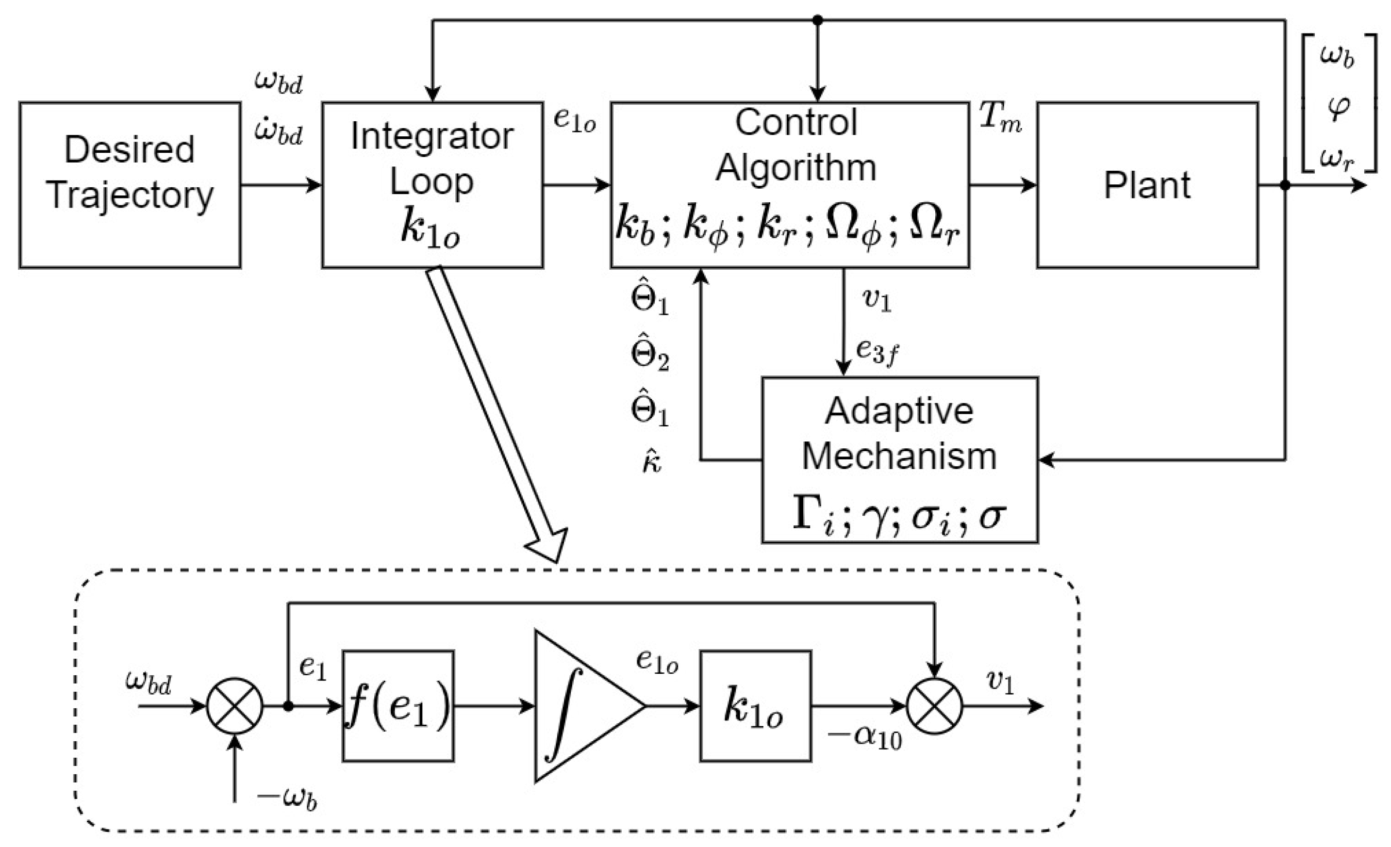
The final scheme of the proposed control system is shown in Figure 1.

4. System Stability and Tuning of the Controller

It follows from the boundedness of approximation errors and filters’ properties that

$$\frac{1}{2}{{\rho }_r}^2+\frac{1}{2}{\left({\rho }_{\phi }+{\epsilon }_b\right)}^2+\frac{1}{2}{\epsilon }_r^2<{\rho }_{max}<\infty .$$

(56)

As all real system parameters are bounded,

$$\frac{{\sigma }_1}{2}{\mathsf{\Theta }}_1^T{\mathsf{\Theta }}_1+\frac{{\sigma }_2}{2}{\mathsf{\Theta }}_2^T{\mathsf{\Theta }}_2+\frac{{\sigma }_3}{2}{\mathsf{\Theta }}_3^T{\mathsf{\Theta }}_3+\frac{\sigma }{2}\kappa <R_{max}<\infty .$$

(57)

Denoting

$$k_{\min }=\min \left\{k_b-\frac{1}{2}, k_{\phi }, k_r-\frac{1}{2}\right\},$$

(58)

$${\sigma }_{\min }=\min \left\{\frac{{\sigma }_1}{2}, \frac{{\sigma }_2}{2}, \frac{{\sigma }_3}{2},\frac{\sigma }{2\kappa } \right\},$$

(59)

$$e^T=\left[v_1,e_{2f},e_{3f}\right], {\vartheta }^T=\left[{\tilde{\mathsf{\Theta }}}_1^T,{\tilde{\mathsf{\Theta }}}_2^T,{\tilde{\mathsf{\Theta }}}_3^T,\tilde{\kappa }\right],$$

(60)

We obtain from (52)

$$\dot{V}\le -k_{1o}f\left(e_1\right)e_{1o}^2-k_{min}{\Vert e\Vert }^2-{\sigma }_{min}{\Vert \vartheta \Vert }^2+{\rho }_{max}+R_{max}.$$

(61)

The component $-k_{1o}f\left(e_1\right)e_{1o}^2$ is negative for $e_{10}\ne 0$ if $k_{1o}f\left(e_1\right)$> 0 and equals 0 if $k_{1o}f\left(e_1\right)=0$. Selecting $k_{1o}=0$ switches the integrator off. In this case, $e_{10}=0, v_1=e_1$ may be taken. The state variables $v_1=e_1, e_{2f}, e_{3f}$ constitute the error system and the controller derivation starts from stage 1. Consequently, the controller structure without the integrator can be obtained from the one derived previously. It is enough to substitute $k_{1o}=0, e_{1o}=0$. If $f\left(e_1\right)=0, k_{1\mathrm{o}}>0,$ the integrator output is “frozen” and kept constant until $f\left(e_1\right)>0$.

Finally, $\dot{V}<0$ for the tracking error $\Vert e\Vert \ge \sqrt{\frac{{\rho }_{max}+R_{max}}{k_{min}}}$ and any parameter error $\vartheta$. On the other hand, $\dot{V}<0$ for parameter error $\Vert \vartheta \Vert \ge \sqrt{\frac{{\rho }_{max}+R_{max}}{{\sigma }_{min}}}$ and any $\Vert e\Vert$.

Summing up: the proposed control causes that the adaptive parameters’ error is uniformly ultimately bounded (UUB) [38] to the compact set:

$$P=\left\{\vartheta : \Vert \vartheta \Vert <\sqrt{\frac{{\rho }_{max}+R_{max}}{{\sigma }_{min}}}\right\}$$

(62)

And the error trajectories are uniformly ultimately bounded to the set:

$$E=\left\{e: \Vert e\Vert <\sqrt{\frac{{\rho }_{max}+R_{max}}{k_{min}}}\right\}.$$

(63)

The bound for $\Vert e\Vert$ may be tightened by increasing $k_{min}$.

It follows directly from the filter Equations (22), (23) and (34), (35) that $e_2$ is bounded if $e_{2f}$ is bounded and $e_3$ is bounded if $e_{3f}$ is bounded. The design parameters ${\mathsf{\Omega }}_{\phi }, {\mathsf{\Omega }}_r$ influence the transient speed and the level of the bound. As $v_1$ and $e_{10}$ are bounded $e_1$ is bounded also. Therefore, the system of state variables $\overline{e}={\left[\begin{array}{ccc}{e}_1& e_2& e_3\end{array}\right]}^T$ is also UUB and the limit set may be tightened by increasing $k_{min}$. Finally, boundedness of the control $T_m$ follows from (46), (47) and the above reasoning.

The final control system is specified by the control law (46), (47), adaptive laws (55), (31), (51), (52), and the errors $v_1, e_{2f}, e_{3f}$ are the controller inputs. Design parameters influencing the system performance are presented in

Table 1. Design parameters of the derived controller.

Notation	Meaning	Main Responsibility
$k_{1o}, f\left(e_1\right)$	Parameters of nonlinear integrator	$\mathrm{Quasi}\text{-}\mathrm{steady}\text{-}\mathrm{state} \mathrm{error} \mathrm{and} \mathrm{the} \mathrm{transient} \mathrm{of} \mathrm{tracking} \mathrm{error} e_1$
$k_b, k_{\phi },k_r$	Gains of the controller	$\mathrm{Transient} \mathrm{of} \mathrm{errors} v_1,e_{2f},e_{3f}$$, \mathrm{volume} \mathrm{of} \mathrm{the} \mathrm{limit} \mathrm{set} \mathrm{for} v_1,e_{2f},e_{3f}$
${\mathsf{\Omega }}_{\phi }, {\mathsf{\Omega }}_r$	Filters’ gains	$\mathrm{Filters}’ \mathrm{dynamics}, \mathrm{filters}’ \mathrm{errors} {\rho }_{\phi }, {\rho }_r$
${\mathsf{\Gamma }}_1, {\mathsf{\Gamma }}_2, {\mathsf{\Gamma }}_3, \gamma$	Adaptive laws’ gains	Speed of adaptation
${\sigma }_1, {\sigma }_2, {\sigma }_3, \sigma$	Adaptive laws’ robustifying coefficients	Boundedness of adaptive parameters
Initial conditions in adaptive laws	Initial guess for adaptive parameters	Transient of adaptive parameters
Initial conditions in filters	Initial guess for stabilizing functions	Transient of filtered variables

. Of course, it is a complicated, nonlinear system, and interactions between any parameter and any signal may be observed, so only the main, dominant “responsibilities” of parameters are presented in Table 1. Parameters of the nonlinear integrator must be selected as a trade-off between the quasi-steady-state error and the oscillatory transient of the tracking error. Increasing controller gains speeds the system up and minimizes the error, but makes the control torque higher. More accurate models (smaller ${\epsilon }_b, {\epsilon }_r$) and faster filters (smaller ${\rho }_{\phi }, {\rho }_r$) decrease ${\rho }_{max}$, so they minimize the effort of the control loop and enhance the tracking accuracy.

The controller design based on the derivation presented in Section 3 is encapsulated in the following steps:

• Choose linear-in-parameters models (3) and (4) for the stiffness and the damping curve and the linear-in-parameters friction models (19) and (42)—the designer has to decide number of adaptive parameters in (21), (42) and select the regressor functions appropriately, as it is demonstrated in (69) in the example below;
• Select the positive error gains $k_b, k_{\phi },k_r$ to obtain the tracking errors decreasing sufficiently fast and to tighten up the bound for $\Vert e\Vert$;
• Choose the filters’ gains ${\mathsf{\Omega }}_{\phi },{ \mathsf{\Omega }}_r$ to obtain sufficiently fast filters and select the adaptation gains ${\mathsf{\Gamma }}_1,{ \mathsf{\Gamma }}_2,{ \mathsf{\Gamma }}_3, \gamma , {\sigma }_1, {\sigma }_2, {\sigma }_3, \sigma$ to make the adaptation fast and robust;
• Complete the closed-loop system consisting of the control law, adaptive laws, and filters.

5. Results

The distinctive features of the proposed approach are demonstrated by a simulation of an exemplary drive with load and motor inertia $J_b=374 \left[{\mathrm{kg} \mathrm{m}}^2\right], J_r=2122 \left[{\mathrm{kg} \mathrm{m}}^2\right]$. Such big values are typical for drilling rigs—parameter $J_r$ contains the so-called rotary table. The friction torques of the motor $T_r$ and load $T_b$ are described by

$$\begin{array}{c}{T}_r\left({\omega }_r\right)=c_r{\omega }_r+T_{fr}\left({\omega }_r\right)=c_r{\omega }_r+\left(T_{cr}+\left(T_{sr}-T_{cr}\right)e^{-{\gamma }_r\left|{\omega }_r\right|}\right)\tanh (100{\omega }_r),\\ T_b\left({\omega }_b\right)=c_b{\omega }_b+T_{fb}\left({\omega }_b\right)=c_b{\omega }_b+W_{ob}{R}_b\left({\mu }_{cb}+\left({\mu }_{sb}-{\mu }_{cb}\right)e^{-{\gamma }_b\left|{\omega }_b\right|}\right)\tanh (100{\omega }_b).\end{array}$$

(64)

The parameters in (61) are: $c_b=50 \left[\frac{Nms}{rad}\right], c_r=425 \left[\frac{Nms}{rad}\right], T_{cr}=150 \left[Nm\right], T_{sr}=400 \left[Nm\right], {\mu }_{cb}=0.5 , {\mu }_{sb}=0.8, {\gamma }_b={\gamma }_r=0.9 \left[\frac{s}{rad}\right] , W_{ob}{R}_b=30 \left[Nm\right].$ The load is typical for drilling—$W_{ob}$ represents the force on the bit and other parameters form the Stribeck-type friction curve.

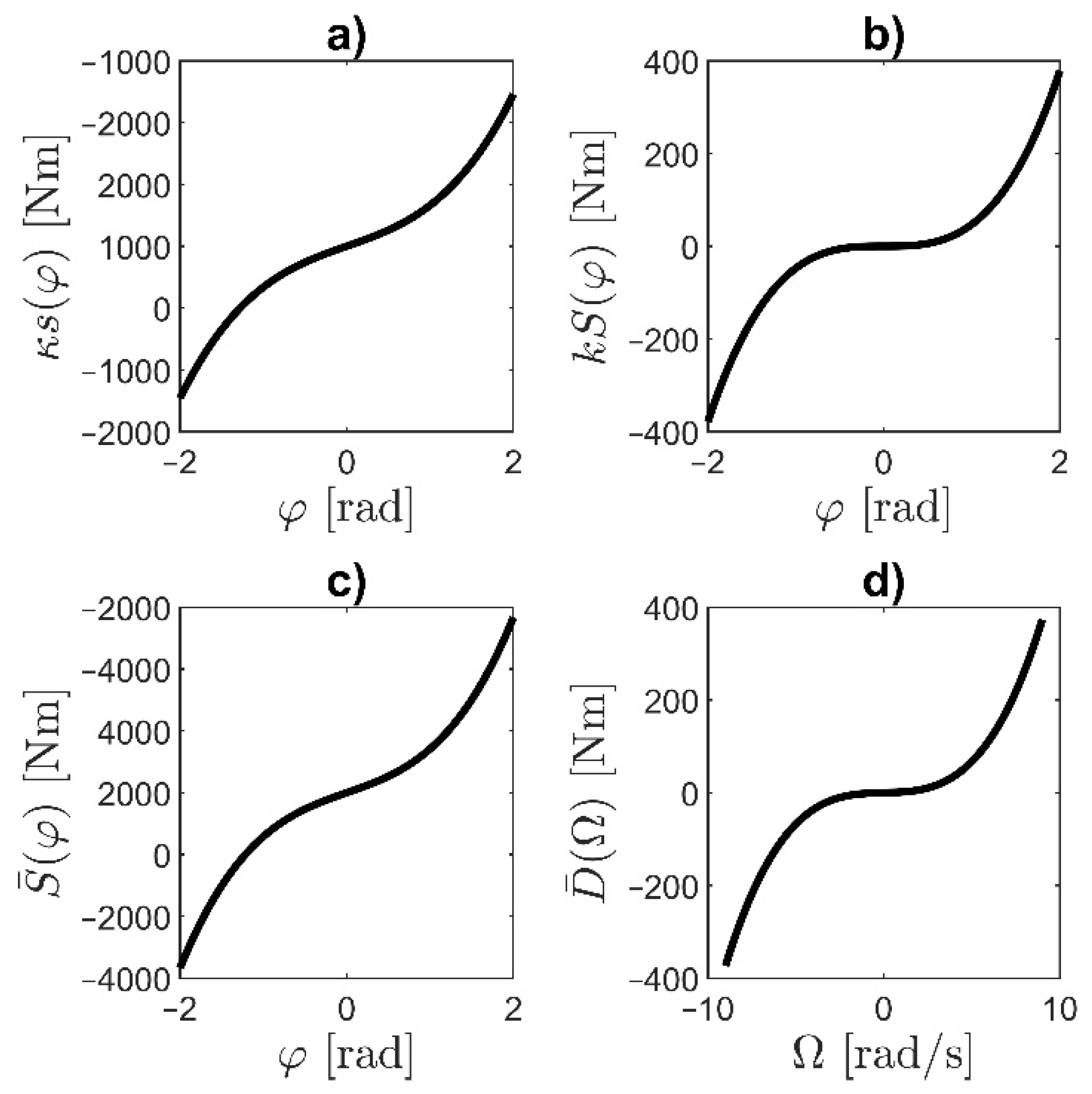
The shaft stiffness torque (3) is given by

$$\overline{S}\left(\phi \right)=\kappa \left(\phi +0.5{\phi }^3\right)=0.5\kappa {\phi }^3+\kappa \phi =kS\left(\phi \right)+\kappa s\left(\phi \right)$$

(65)

And damping (4) by

$$\overline{D}\left(\mathsf{\Omega }\right)=c\left(\mathsf{\Omega }+0.5{\mathsf{\Omega }}^3\right)=cD\left(\mathsf{\Omega }\right)$$

(66)

And unknown values of parameters are $\kappa =473 , c=1$(in proper units). Functions $S\left(\phi \right)$ and $s\left(\phi \right)$ represent designer’s knowledge of the stiffness curve. The function $s\left(\phi \right)$ (known, nonlinear component of the stiffness torque) which is used as the virtual control, is modeled taking

$$s\left(\phi \right)=\phi +0.4{\phi }^3$$

(67)

And function $S\left(\phi \right)$ by

$$S\left(\phi \right)={\phi }^3$$

(68)

So, the unknown value of the last parameter is $k=0.1\kappa$. The functions: $\overline{S}\left(\phi \right)$, $kS\left(\phi \right)$, $\kappa s\left(\phi \right)$, $\overline{D}\left(\mathsf{\Omega }\right)$ are shown in Figure 2.

The regressor functions ${\xi }_1, {\xi }_2$ (according to (20)) and ${\xi }_3$ (according to (42)) are defined as

$$\begin{gathered} {\xi }_1^T=\left[\begin{array}{cc}D\left(\text{Ω}\right)& S\left(\phi \right)\end{array}\right], \\ {\xi }_2^T=\frac{1}{\breve{\kappa }}\left[{\breve{J}}_b\begin{array}{cccc}\left({\dot{\omega }}_d+k_{1o}f\left(e_1\right)e_1\right)& {\breve{c}}_b{\omega }_b& {\breve{T}}_{cr}\tanh (100{\omega }_b)& \left({\breve{T}}_{sr}-{\breve{T}}_{cr}\right)\tanh (100{\omega }_b)e^{-{\breve{\gamma }}_b\left|{\omega }_b\right|}\end{array}\right], \\ {\xi }_3^T=\frac{1}{\breve{\kappa }}\left[{\breve{J}}_r\begin{array}{cccc}{\text{Ω}}_3\left({\alpha }_r-{\alpha }_{rf}\right)& {\breve{c}}_r{\omega }_r& {\breve{W}}_{ob}{\breve{R}}_b{\breve{\mu }}_{cb}\tanh (100{\omega }_r)& {\breve{W}}_{ob}{\breve{R}}_b\left({\breve{\mu }}_{sb}-{\breve{\mu }}_{cb}\right)\tanh (100{\omega }_r)e^{-{\breve{\gamma }}_r\left|{\omega }_r\right|}\end{array}\right], \end{gathered}$$

(69)

where any variable with the sign $\stackrel{ˇ}{}$ denotes the initially assumed, unknown value of the parameter, for instance, ${\breve{J}}_b$ is the initial guess for $J_b$. This selection of the regressor functions is a consequence of the friction model used in the design. The average difference between the actual parameter and the initial guess is 20% and the initial value of each adaptive parameter is equal to 80% of the real value. The controller parameters are chosen as: $k_{1o}=5, k_b=30, k_{\phi }=30, k_r=30, {\mathsf{\Gamma }}_1=diag\left({10}^{-4};1\right), {\mathsf{\Gamma }}_2=diag\left(0.1;0.1;0.1;0.1\right), {\mathsf{\Gamma }}_3=diag\left({10}^{-3};{10}^{-3};{10}^{-3};{10}^{-3}\right), \gamma =2·{10}^{-3}$, ${\sigma }_1={\sigma }_2={\sigma }_3=\sigma ={10}^{-3}$, while the filter parameters are: $a_{\phi }=a_r={10}^2, z_{\phi }\left(0\right)=z_r\left(0\right)=0$.

The step response of the plant is shown in Figure 3. The plant corresponds to the drilling rig with parameters taken from [20,31]. We can observe the oscillatory character of two-mass resonant systems. As the moments of inertia $J_b, J_r$ are quite big, the plant is rather slow. Strongly nonlinear friction also contributes to high amplitude oscillations visible during the first 40 s of the step response. All these unacceptable phenomena will be eliminated by the proposed controller.

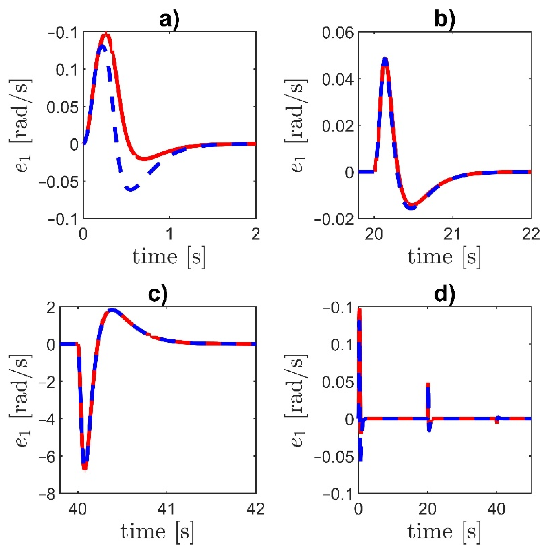
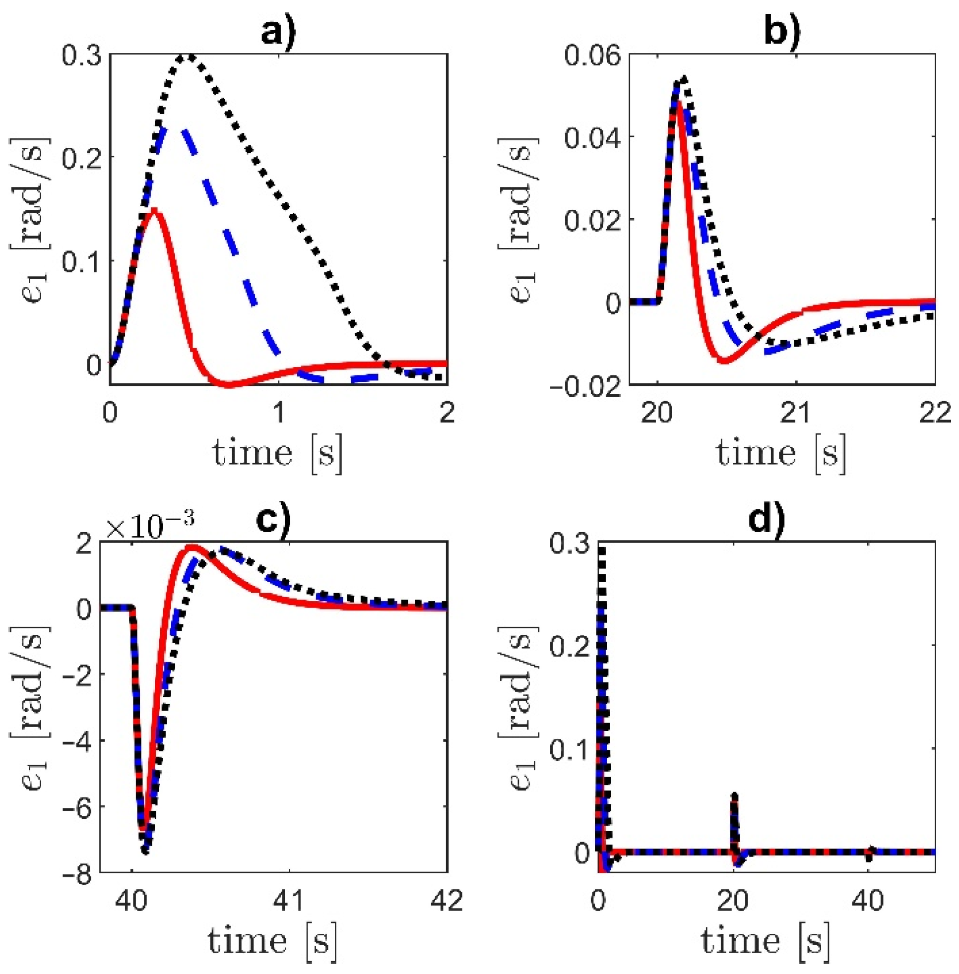
In the first experiment, the tracking of the reference trajectory is studied. The reference speed is not constant. Initially, the reference speed ${\omega }_{bd}$ starts from 0 to $15\left[\frac{\mathrm{rad}}{\mathrm{s}}\right]$. At $t=20 \left[\mathrm{s}\right]$ ${\omega }_{bd}$ is changed from $15\left[\frac{\mathrm{rad}}{\mathrm{s}}\right]$ to $30\left[\frac{\mathrm{rad}}{\mathrm{s}}\right]$. For the end, at $t=40 \left[\mathrm{s}\right]$, the speed ${\omega }_{bd}$ is changed from $30\left[\frac{\mathrm{rad}}{\mathrm{s}}\right]$ to $20\left[\frac{\mathrm{rad}}{\mathrm{s}}\right]$.

In this experiment two controllers are compared:

• Controller LI with a linear integrator—$k_{1o}>0, f\left(e_1\right)=1$;
• Controller NI with a nonlinear integrator gain—$k_{1o}>0, f\left(e_1\right)=1-\tanh \left(K{e}_1^2\right)$.

Parameter $K$ modifies the shape of the nonlinear anti-wind-up factor $f\left(e_1\right)$. For the presented results $K=100$ is applied.

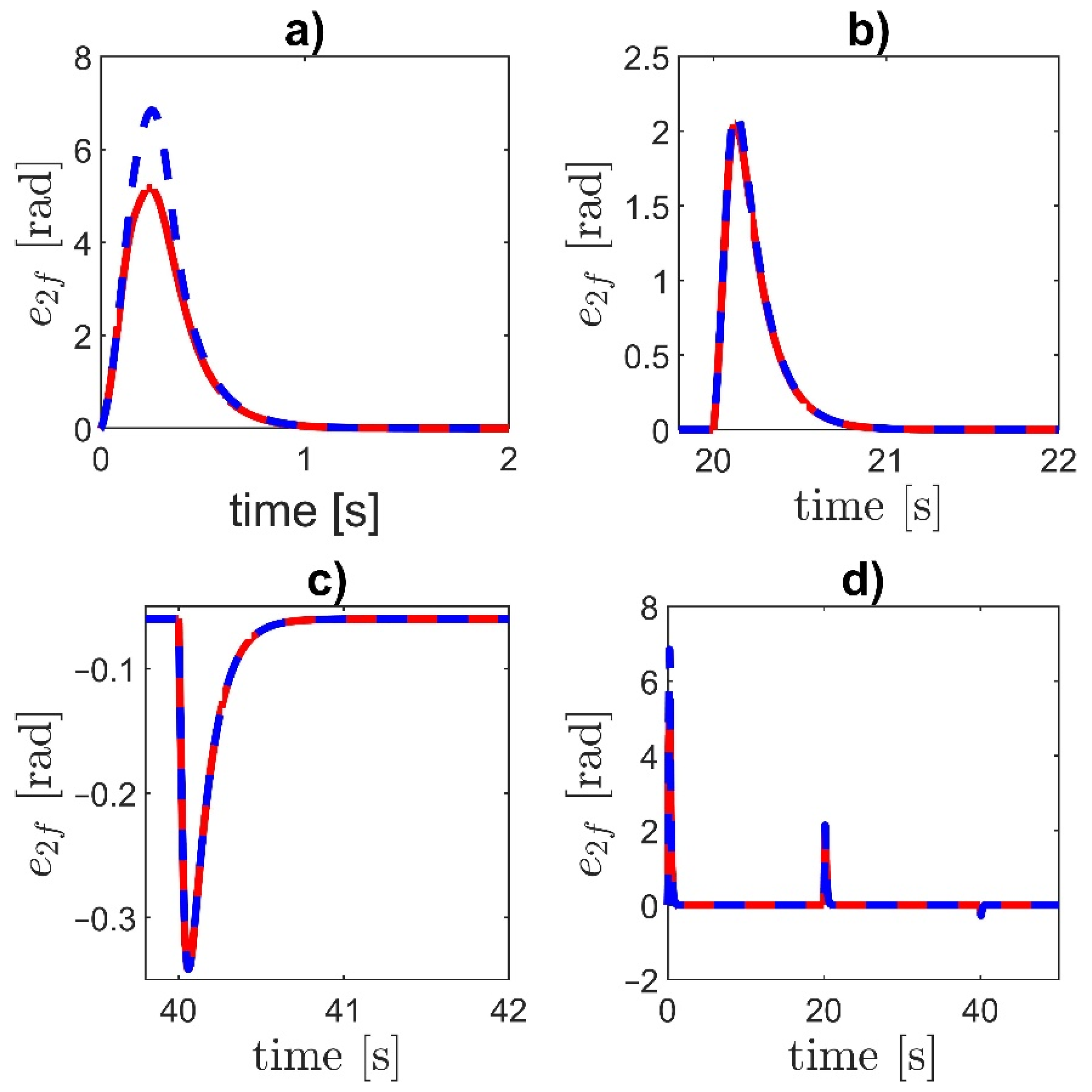
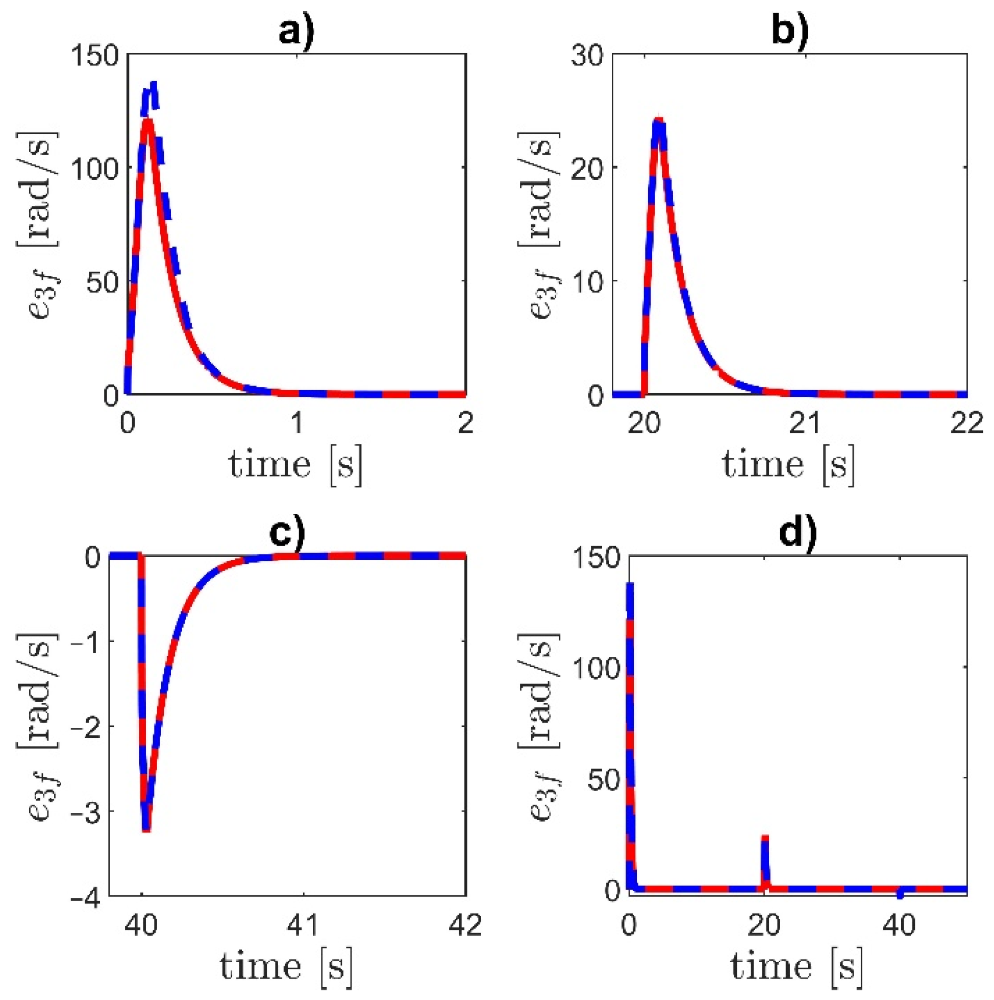
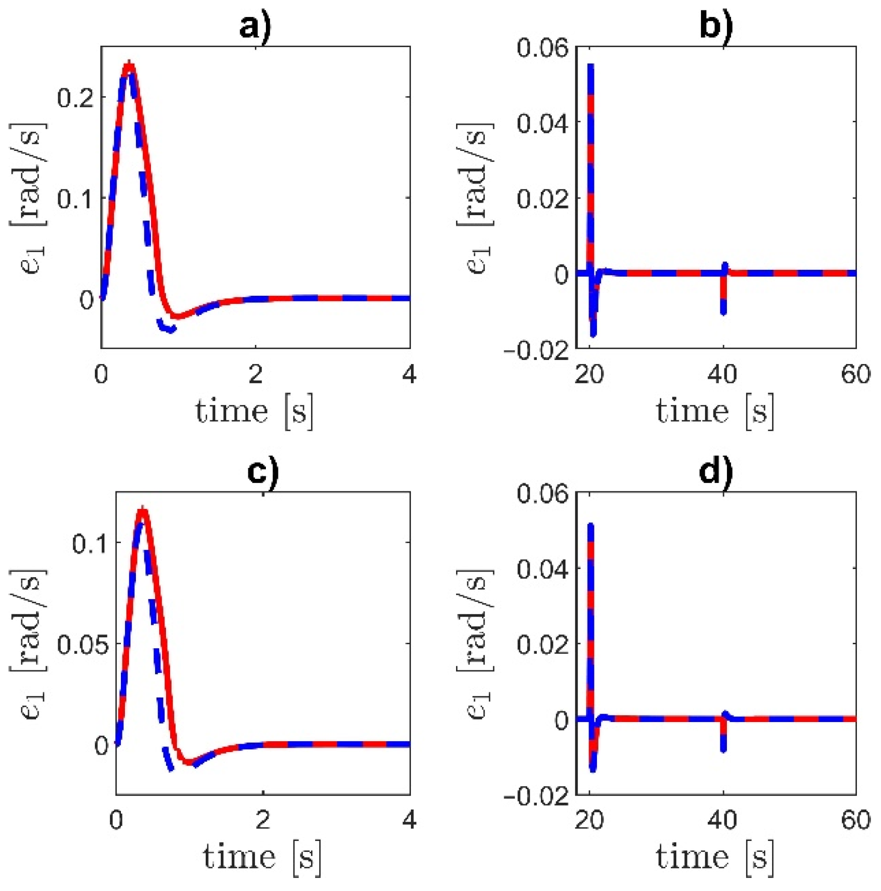
Figure 4 demonstrates the tracking error $e_1$ for both controllers. Filtered errors $e_{2f}$ and $e_{3f}$ are shown in Figure 5 and Figure 6. The initial part of the transient and the response to the step changes occurring at $t=20 \left[\mathrm{s}\right]$ and $t=40 \left[\mathrm{s}\right]$ are plotted, and finally the complete trajectory is given.

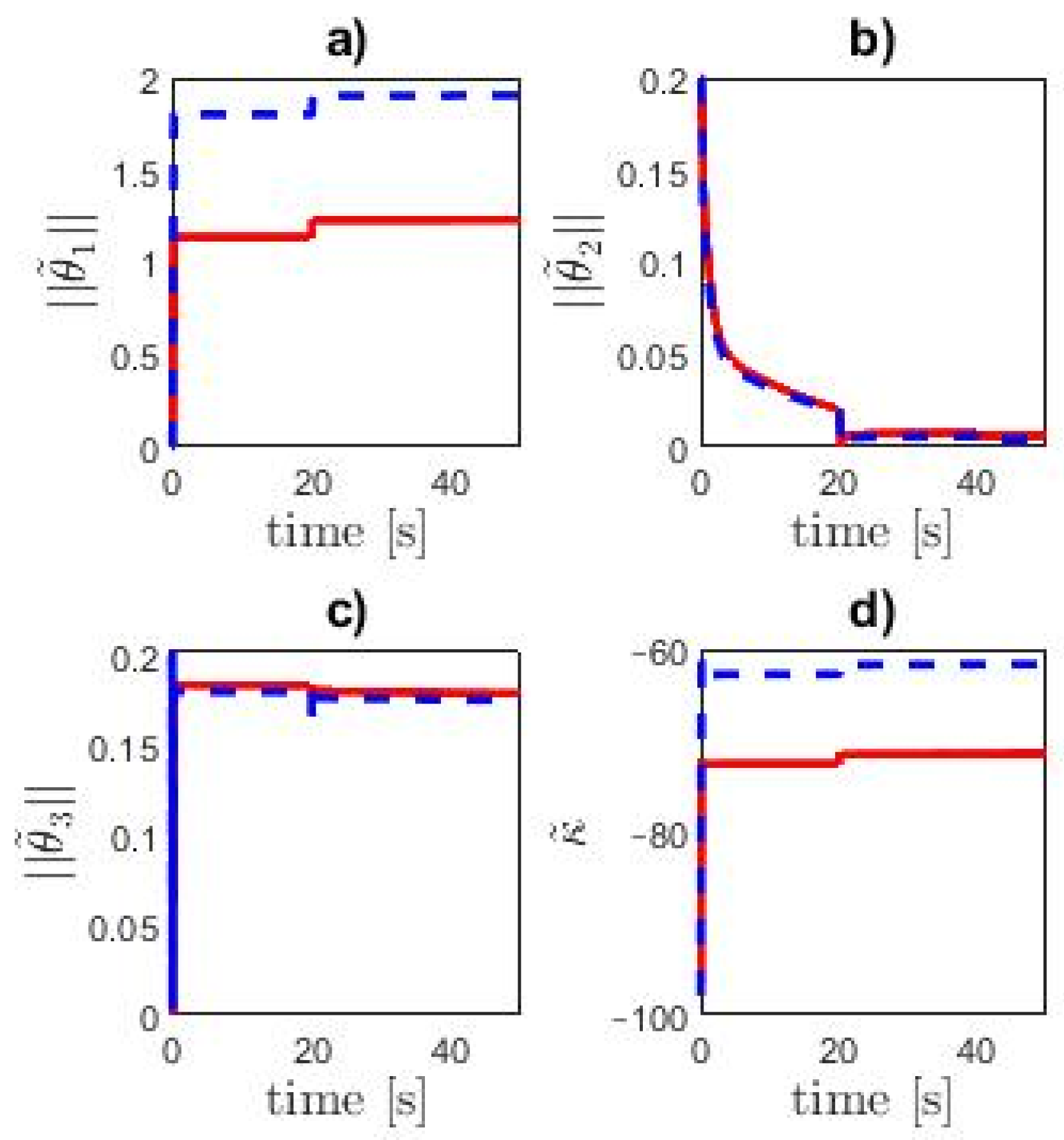
Controller NI provides a smaller velocity overshoot than the controller with the linear integrator. Errors of adaptive parameters are shown in Figure 7. For both controllers, the adaptive parameters remain bounded.

In the second experiment the system robustness against the unmodeled dynamics is tested. The unmodeled dynamics describes a current control loop that generates electromagnetic torque. The first-order transfer function

$$G\left(s\right)=\frac{1}{Ts+1}$$

(70)

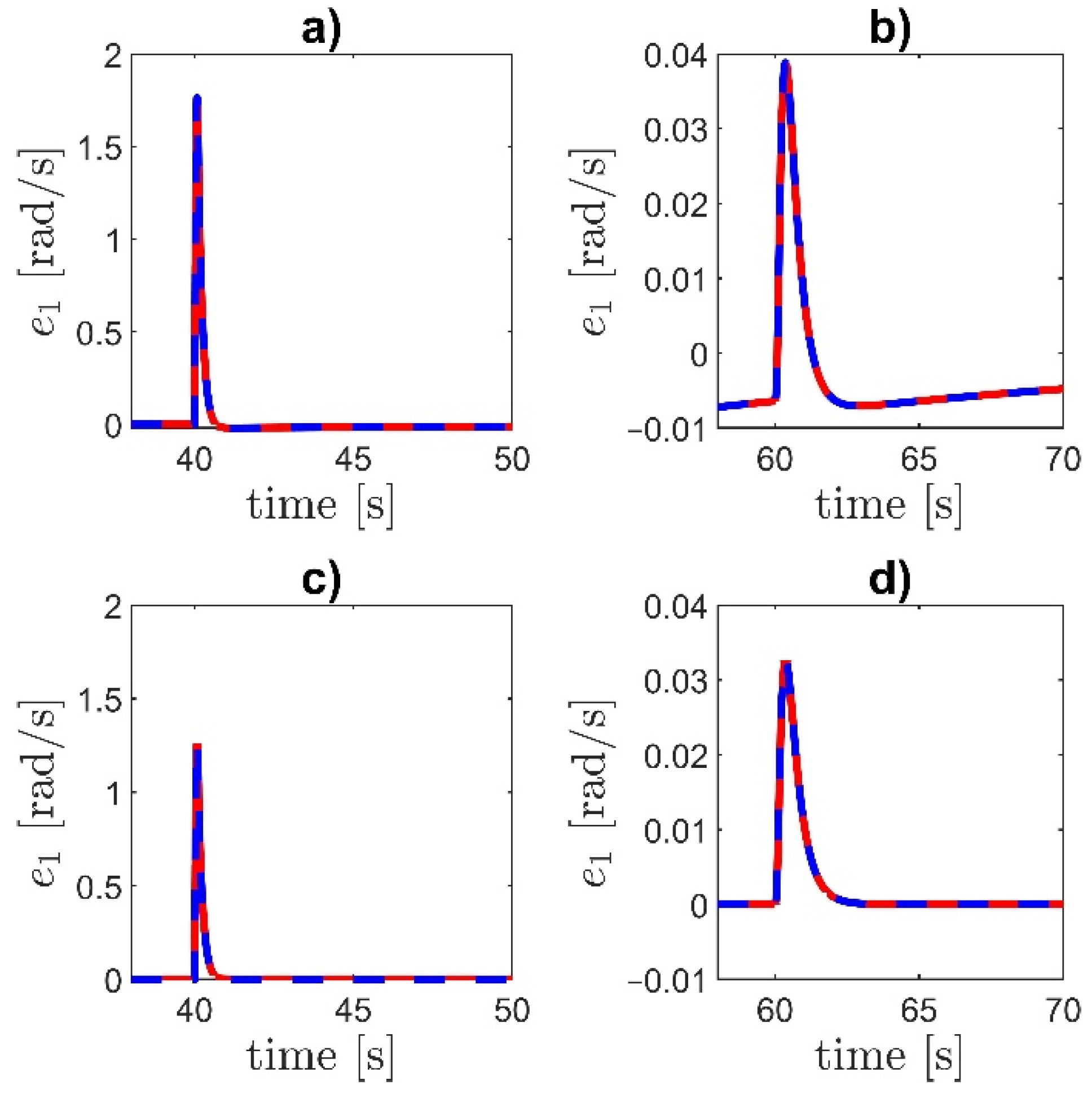
is used to model current-control loop. The speed reference and the controller parameters remain the same as in the first experiment. Figure 8 and Figure 9 demonstrate the tracking error $e_1$ for different values of a time constant $T$. The initial part of the transient and the response to the step changes at $t=20 \left[\mathrm{s}\right]$ and the complete time-history are plotted.

As we can see, the proposed controllers are robust to unmodeled dynamics in a wide range of changes of a time constant $T.$ The control system is stable. Good tracking and transient performances are maintained.

The aim of the third experiment is to demonstrate the robustness of the proposed controller against friction changes. The drive is started knowing the actual values of friction parameters. The constant reference speed ${\omega }_{bd}=10 \left[\frac{\mathrm{rad}}{\mathrm{s}}\right]$ is applied. At time $t=40 \left[\mathrm{s}\right]$ the $W_{ob}$ value was increased achieving $180\%$ of the nominal value and at $t=60 \left[\mathrm{s}\right]$ the $T_{cr}$ value was increased to 140% of the nominal value. The simulation results are presented in Figure 10.

The drive system is working correctly. The reaction of the control system to a change of $W_{ob}$ is faster than to a change of $T_{cr}$. If the adaptation is switched off, the maximum values of the tracking error are bigger and the change of $T_{cr}$ results in increasing the tracking error (Figure 10b). The integrator in the outer loop makes the system stability robust against the change of $W_{ob}$, even without the adaptation. Enabling adaptation decreases the maximum tracking error, maintains UUB stability according to the derivation, and reduces the quasi-steady-state tracking error for any change of plant parameters.

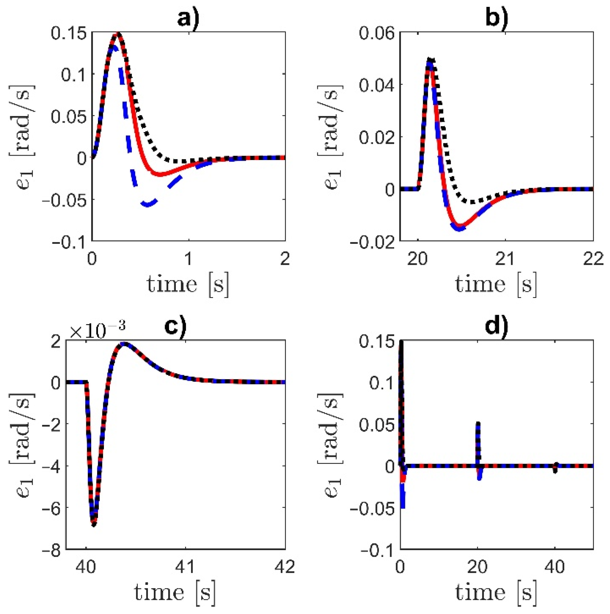
In the fourth experiment, the influence of the parameters $k_b, k_{\phi },k_r, k_{1o}$ (error gains) and $K$ (which modifies the shape of the nonlinear anti-wind-up factor) is tested. The speed reference and the controller parameters remain the same as in the first experiment. Figure 11, Figure 12, Figure 13, Figure 14 and Figure 15 demonstrate the tracking error $e_1$ for different values of the parameters $k_b, k_{\phi },k_r, k_{1o}$ and $K$. The initial part of the transient and the response to the step changes at $t=20 \left[\mathrm{s}\right]$ and $t=40 \left[\mathrm{s}\right]$ are shown.

Increasing the value of $k_{1o}$ increases the overshoot but decreases the settling time. The decrease in the parameter $k_b, k_{\phi },k_r$ increases the maximal error $e_1$ and causes that the convergence is slower. For higher values of the parameter $K$, the error overshoot is smaller.

6. Conclusions

An adaptive control problem was formulated and solved for a two-mass drive system with a flexible shaft in the presence of nonlinear stiffness and damping. The proposed model of the plant allows the consideration of special applications, with peculiar couplings and highly nonlinear friction affecting both ends of the shaft. All parameters of the model are unknown. The field of potential applications ranges from nano-drives, through various robotic industries, to huge oil rigs used in the gas and oil industry.

The proposed approach was based on several modifications of adaptive backstepping. Although the considered system is not in the strict-feedback form, the recurrent design procedure is proposed. This ‘recurrency’ of the design offers a very convenient, systematic way to derive the final controller. The presented methodology:

• Allows avoiding overparameterization (the number of adaptive parameters is the same as the number of unknown parameters) by the application of the tuning functions technique;
• Prevents the “explosion of complexity” in the control law—as a result of smart filter application;
• Provides robust adaptation by the use of robust adaptive laws;
• Minimizes the quasi-steady-state tracking error, unavoidable in the presence of the applied approximations, by the implementation of the nonlinear PI controller in the initial loop.

The Lyapunov function technique is used to perform the rigorous proof of the closed-loop system stability in the UUB sense. The properties of the derived controller depend on a few parameters that are easy to tune. The design and tuning procedures are described in detail.

The introduction of the nonlinear integrator at the first stage of the controller design is the original solution used in this research. Nonlinear integrator helps to decrease the quasi-steady-state tracking error and mitigate high control values and output oscillations. The selection of a particular shape of nonlinear integrator gain depending on the actual tracking error allows to trade-off between the control extremal values and tracking error bounds. The presented derivation also includes the system without the additional integrator in the initial loop. This is obtained by taking the integrator gain $k_{1o}=0$.

As it was tested, the same design approach is able to suppress the shaft oscillations and compensate for nonlinear friction or any other resistance torques. The presented controller is sufficiently accurate from a practical point of view. It was demonstrated that the proposed controller works properly even if some assumptions of the derivation are violated. For instance, the closed-loop system is robust against the unmodeled dynamics of the torque/current control loop.

The proposed design procedure may be easily generalized for multi-mass systems or models, including the current control loop. It is also possible to consider state constraints as in [39]. The proposed model is commonly accepted in the literature under two assumptions: (1) the inertia of the shaft is evidently smaller than the inertia of the motor and the load, and (2) torsional oscillations in a shaft of moderate length are considered. The interesting question is: what happens if we apply the controller derived from the inaccurate ODE model to the plant that should be rather described by a more accurate PDE model. This interesting topic will be investigated in our future research.