Sensorless Speed Control of Brushed DC Motor Based at New Current Ripple Component Signal Processing

Abstract

Signal processing of the brushed DC motor current was developed in this paper to obtain information about a rotor speed from a measured motor current. The brushed DC motor current contains a signal with a frequency proportional to the rotor speed. This signal is the outcome of a commutation process occurring in the brushed DC motor, and it is called a ripple component. Since the number of ripples in the measured motor current per one rotation is constant, the rotor speed can be estimated. A discrete bandpass filter with a floating bandwidth was developed as the main part of signal processing. This new interpretation of the bandpass filter was used to extract a frequency of the ripple component from the measured motor current. This frequency was used to acquire information about the estimated rotor speed. The estimated speed was set as a feedback value to a cascade control structure to provide sensorless speed control. The advantages and limitations of this approach are presented in this paper. Based on simulations and experimental results, it was confirmed that the proposed sensorless speed control is robust, accurate, and works precisely in a wide range of speeds.

1. Introduction

The advancement of technology and automation has led to the widespread use of electric motors in many applications. Brushed DC motors are used in various industrial sectors and a wide range of consumer products such as pumps, air fans, and so on. These drives are also commonly used in the automotive industry, as automobile starters, window lifters, windshield wipers, etc. However, brushed DC motors require more attention to maintenance due to the commutator and brushes. The mechanical commutator is the most vulnerable component and the main practical problem of these motors. This component may also limit the maximum speed of the DC motor due to its mechanical endurance. A mechanical sensor coupled to a motor shaft is required to obtain information about the speed or position of the motor. Sensors such as the resolver, encoder, Hall effect sensor, and tachometer are commonly used. However, the overall cost of a DC drive system increases significantly with the addition of such a sensor, which is prone to failure in industrial environments. The sensor reliability is remarkably affected by environmental conditions that the sensor is exposed to, such as dust, pollution, vibrations, and temperature. A sensorless speed or position estimation can be used to minimize the cost and issues associated with the sensors in a DC drive system. The main advantages of the removal of such sensors and using a sensorless algorithm are decreased maintenance, decreased drive volume, a reduced number of connections, and a reduced cost of the final system. The sensorless algorithms are also used as a redundant solution in case of a sudden failure of the mechanical sensor. These algorithms can be divided into two groups: those based on the dynamic model of the DC motor and those based on the ripple component of the motor current.

The methods based on the dynamic model of DC motor depend on the parameters of the brushed DC motor such as the resistance, inductance, and back-emf constant. However, these parameters are not constant, and they vary under different operational conditions, for example, with temperature. Varying parameters then lead to uncertainty in speed estimation. Nevertheless, these parameters can be estimated dynamically [1], but this approach usually leads to a nonlinear model, which is more difficult, and increased computational time is required. Some techniques indirectly model a motor with the use of neural networks [2] or the Kalman filter [3]. The combination of neural networks and Sliding mode control was used in [4]. Sensorless speed control for very small, brushed DC motors with an adaptive estimator was presented in [5].

The methods based on the ripple component of motor current do not require any knowledge of motor parameters to obtain information about the rotor speed because the motor current already contains this information. The measured motor current is mainly composed of two components: a DC component and an AC component, also known as the ripple component. The DC component is responsible for providing torque to the motor, and its amplitude depends on a motor load. The AC component is created by converting the DC current supplied by a stationary source into an AC current in an armature coil by the commutator and brushes. It should be noted that the AC component contains a ripple, which is directly proportional to the rotor speed. According to the fact that the number of ripples in the measured motor current per one rotation is constant, the rotor speed can be estimated. There are some methods that use the ripple component of the brushed DC motor to estimate the rotor speed.

An adaptive filter was used to estimate the rotational speed in [6], specifically Adaptive Line Enhancer (ALE). Simulation studies of the ALE are presented within the paper but without experimental verification. The authors stated in the paper that they would like to examine the range and the accuracy of the estimated speed as well as the load effect in practice.

The support vector machines were applied in [7], where the rotor speed was estimated by using the inverse distance between the detected pulses, and the position was estimated by counting all detected pulses. The paper shows good results, but there is no explanation for why the results were not presented for the low speeds, specifically under 501 rpm. In the paper, a response of the proposed method to the applied load is not available either. The paper presented an interesting sensorless method with speed detection from ripple current but without controlling the speed. The complexity of the proposed method also requires a microcontroller with higher computational power, due to plenty of mathematical operations.

The method based on measuring the inductive spikes generated when the motor is turned off was proposed in [8]. The estimated speed was used as a feedback value to the speed controller, while the speed was measured in steady state. The authors declare that it would be of great interest to have an analysis of dynamic behavior and how to optimize a speed controller.

Another approach [9] used the spectral components of the motor current. This method is also useful for the brushed DC motors with a large number of coils where the ripple component is almost negligible. The proposed method was tested within a small speed range, specifically from 2000 rpm to 3000 rpm, without a control structure. The proposed method contains a lot of mathematical operations, which could lead to higher computational requirements.

Texas Instruments made an application note [10] where an analog bandpass filter was used to count ripples in the form of pulses, which requires the use of additional hardware. This approach used the pulse counting technique without controlling the motor speed or position.

Microchip made a similar application note [11], where a ripple counting technique was proposed. They also provide a software implementation of the proposed sensorless method to the microcontroller unit. The main goal of this counting implementation is to count all the ripples until the number of expected ripples is reached. This approach is very suitable to control the motor position by counting pulses. However, a way to control the rotor speed was not the scope and purpose of the application note, so it was not presented.

In [12], the comparison between the model-based and non-model-based methods is presented. The model-based methods experimentally verified in this article are specifically the pseudo-sliding mode observer and the observer with a PI controller. However, limited accuracy was detected for these methods. According to this fact, they were compared to the non-model-based method, which is deeply investigated in this article.

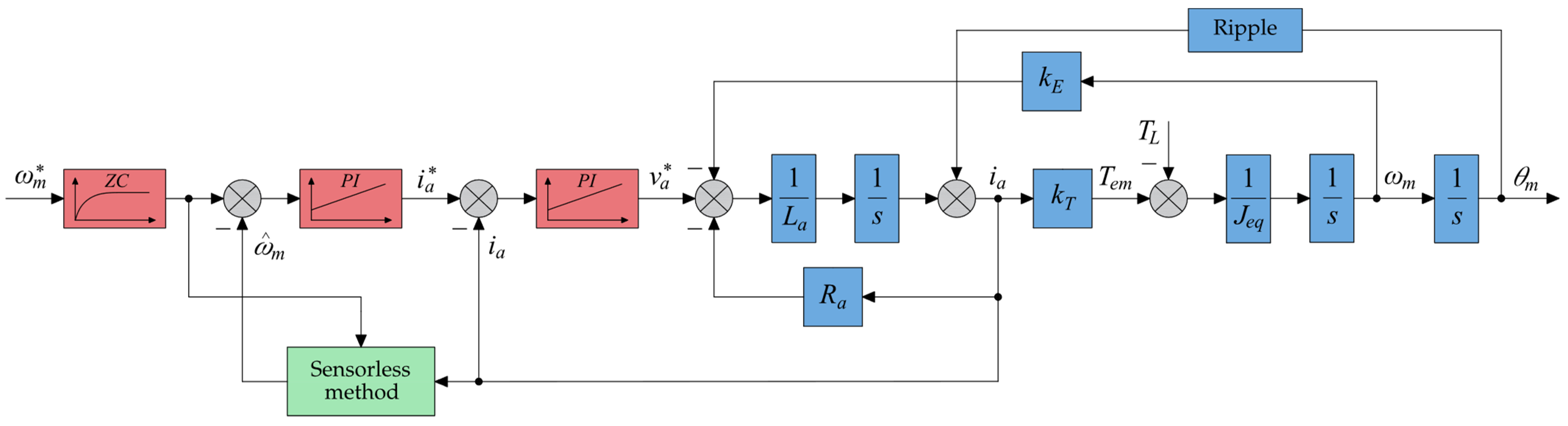
The above-mentioned methods have shown some advantages and disadvantages. The main idea of this paper is to provide low-cost sensorless speed control of brushed DC motor independent of the motor parameters. In the above-mentioned methods, there was not a clear statement about the motor operation at low speeds. This article provides an analysis of the proposed sensorless method in the whole speed range. The method of optimizing the controllers will be also revealed, as well as a detailed analysis of the ripple occurrence in the brushed DC motor current. The main parts of the current ripple signal processing are composed of a discrete bandpass filter with floating bandwidth, discrete comparator, and timer peripheral on the microcontroller unit. The discrete bandpass filter with floating bandwidth as well as the discrete comparator will be used to perform the conversion of the ripple current to the pulses. Afterward, pulses will not be counted, but their length will be measured with a timer peripheral to estimate the rotor speed. The estimated speed will be used as a feedback value for a speed controller. The cascade control structure with the speed and current controller is used to provide sensorless speed control.

2. Ripple Component of Brushed DC Motor Current

In this section, the dynamic model of the DC motor with the mathematical expressions is given. Moreover, the reason standing behind the presence of ripple in the measured brushed DC motor current will be presented as well as the analysis of the ripple component in time and frequency domain.

2.1. Dynamic Model of DC Motor

The system structure of the DC motor is depicted as employing an equivalent circuit in Figure 1, including the armature resistance $R_a$ and the armature inductance $L_a$.

The equivalent circuit shows the conversion between the electrical and the mechanical power. In this figure, the armature current $i_a$ is flowing. This current produces the electromagnetic torque $T_{em}$ necessary to rotate the mechanical load at the angular velocity of ${\omega }_m$. Across the armature terminals, the rotation at the speed of ${\omega }_m$ induces a voltage called the back-emf $e_a$. On the electrical side, the armature voltage $v_a$ overcomes the back-emf and causes the current to flow. As the current flows across the armature winding resistance and the armature winding inductance, the equation for the electrical side of the DC motor with the use of Kirchhoff’s voltage law can be written as follows:

$$v_a=R_a{i}_a+L_a\frac{d{i}_a}{dt}+e_a$$

(1)

The back-emf is proportional to the angular velocity of the rotor, expressed as:

$$e_a=k_E{\omega }_m$$

(2)

where $k_E$ is the back-emf constant. On the mechanical side of the DC motor, the electromagnetic torque produced by the motor overcomes the load torque $T_L$ to produce acceleration. The equation for the mechanical side is shown as:

$$T_{em}-T_L=J_{eq}\frac{d{\omega }_m}{dt}$$

(3)

where $J_{eq}$ is the total effective value of the combined inertia of motor $J_M$ and the inertia of the mechanical load $J_L$. The electromagnetic torque is proportional to the armature current, which yields to the following equation:

$$T_{em}=k_T{i}_a$$

(4)

where $k_T$ is the motor torque constant, which is the same as the back-emf constant. Equations (1)–(4) are the basic equations of the DC motor related to the equivalent circuit in Figure 1. It should be noted that the equations of the electrical and mechanical system are coupled. The back-emf in the electrical system equation depends on the mechanical speed and the electromagnetic torque in the mechanical system equation depends on the electrical current. The electrical power absorbed from the electrical source by the motor is converted into mechanical power and vice versa. In steady state, when the voltage $V_a$ is applied, the voltage drop across the armature winding inductance is no longer considered, and the following equations for the armature current and the angular velocity of the rotor are derived:

$$I_a=\frac{T_{em}}{k_T}$$

(5)

$${\omega }_m=\frac{V_a-R_a{I}_a}{k_E}$$

(6)

To investigate the dynamic behavior of DC motor it is necessary to express the motor equations as a system of differential equations:

$$\frac{d{i}_a}{dt}=\frac{1}{L_a}\left(v_a-R_a{i}_a-k_E{\omega }_m\right)$$

(7)

$$\frac{d{\omega }_m}{dt}=\frac{1}{J_{eq}}\left(k_T{i}_a-T_L\right)$$

(8)

According to these equations, a block diagram including both the electrical and mechanical system of DC motor is established and shown in Figure 2.

However, the dynamic model of the DC motor as shown in Figure 2, does not include the effect of the commutation, and the current ripple is not presented. The current ripple gives an insight into a commutation process occurring in the brushed DC motor. To understand the presence of the current ripple, the principle of the commutation process will be introduced.

2.2. Commutation Process of Brushed DC Motor

Considering the elementary brushed DC motor with four commutator segments and two brushes, as illustrated in Figure 3, the commutation process will be divided into three intervals based on the mechanical position of the rotor ${\theta }_m$. In the first interval (Figure 3a), the current flows across the brush with a positive power supply and both parallel circuits to the brush with a negative power supply. The next interval occurs when the brushes short-out two adjacent commutator segments (Figure 3b), which results in the current circulating between the segments. These two segments are interconnected with the one armature coil represented by the inductance. When the adjacent commutator segments are shorted out, it will lead to a short-circuit of the corresponding armature coil, with no current flowing through it. When this situation occurs, the inductance is no longer part of the circuit, which leads to a reduction of the armature impedance, thus causing the overall current to rise and create the current ripple. In this region, the corresponding coil undergoes commutation, where its current direction reverses as the rotor turns further. After a sudden shorting out, the last interval occurs. In the last interval (Figure 3c), the circuit is composed of four coils again, thus a larger impedance, which leads to the sudden decrease of the current, and the ripple component is presented. The periodic shifting of coils under the brushes, as the rotor turns, produces the periodic current ripple, which is proportional to the rotor speed. According to the fact that the number of ripples in the current per one rotation is constant, the speed of the brushed DC motor can be estimated.

There is also another case when the influence of commutation on the motor current is slightly different. The previous case was focused on the machine with an even number of commutator segments. There are some differences when the number of commutator segments is odd. The principle will be shown in Figure 4 when the brushed DC motor with three commutator segments is illustrated.

The commutation process will be divided into three intervals based on the mechanical position of the rotor. The principle is similar to the previous case. The difference between these two cases can be seen if we compare Figure 3b with Figure 4b, which is the interval when some of the armature coils are short-circuited. During this interval in Figure 3b, armature coil 1 and the opposite armature coil 3 are short-circuited, while in Figure 4b, there is just one armature coil to be short-circuited because there is no coil on the opposite side. The important fact is that armature coil 1 in Figure 4b will be also shorted-out by a second brush, thus providing two ripples per one mechanical rotation, while armature coil 1 in Figure 4a is in opposite with armature coil 3 and the ripples produced by these two coils will be counted into one ripple. According to these facts, the brushed DC motor in Figure 3 with an even number of commutator segments will create four ripples per one mechanical rotation, while the motor in Figure 4 will create six ripples per one mechanical rotation. The number of ripples per one mechanical rotation can be calculated by the following equation:

$$number of ripple{s}_{rot}=c·k·p$$

(9)

where $c$ is the coefficient contingent to the parity of the number of commutator segments $k$, with $c=1$ when $k$ is even and $c=2$ when $k$ is odd and $p$ is the number of pole pairs.

When comparing these two types of constructions concerning the number of commutator segments, the following statements for the odd number of segments are given:

• produce twice as many ripples;
• decrease the length of a commutation interval;
• current flowing into the commutator will not divide evenly into the parallel circuits;
• produce the ripples with a smaller amplitude.

It is worth mentioning, that the ripple in the current can be also reduced by increasing the number of coils and slots. This fact yields to the following statement. The brushed DC motors with a small number of coils and commutator segments have a significant ripple in the motor current. Otherwise, the brushed DC motor with a large number of coils and commutator segments has a very small ripple. In other words, the motor current just consists of the DC component. This leads to very difficult processing of such a small signal to correctly estimate the rotor speed from the measured brushed DC motor current.

Figure 5 shows the measured motor current of the brushed DC motor. This motor will be used for the experimental verifications. The current was measured with a current probe on an oscilloscope. The figure shows the comparison between measured motor current with pulse width modulation (PWM), which affects the current ripple with higher harmonics and without PWM modulation at a rotational speed of 3000 rpm. The figure also illustrates when the rotor reaches one mechanical rotation. This information can be determined by knowledge of the motor parameters related to the commutation process. These are presented in

Table 1. Parameters of brushed DC motor related to the commutation process.

Parameter	Symbol	Value
Number of pole pairs	$p$	1
Number of commutator segments	$k$	8
Coefficient of the parity	$c$	1

.

As we can see from the picture, one mechanical rotation is given by eight ripples in the motor current. The distance between the first and the last ripple is about 0.02 s. Having this information, the rotational speed can be calculated by the following equation:

$$n_m=\frac{60}{T}=\frac{60}{0.02}=3000 rpm$$

(10)

To extract information about the rotor speed from the measured motor current (Figure 5), it is necessary to know the exact frequency of the current ripple. The frequency of the current ripple $f_r$ can be calculated by the following equation from [13]:

$$f_r=\frac{c·k·p·n_m}{60}$$

(11)

where $n_m$ is the rotational speed. Equation (11) yields that, for determining an accurate value of the current ripple frequency, it is necessary to know the number of commutator segments and number of pole pairs. These parameters are constant, and they depend on the motor construction, thus they are not changing during motor operation. Assuming the parameters of the brushed DC motor from Table 1 that are used to perform an experimental verification and the rotational speed calculated by Equation (10), we will obtain the following frequency of the current ripple:

$$f_r=\frac{c·k·p·n_m}{60}=\frac{1·8·1·3000}{60}=400 \mathrm{Hz}$$

(12)

By performing Fast Fourier Transform (FFT) of motor current with PWM at a given speed, the frequency of current ripple is presented in a frequency domain as calculated (Figure 6 and Figure 7):

3. Proposed Sensorless Method

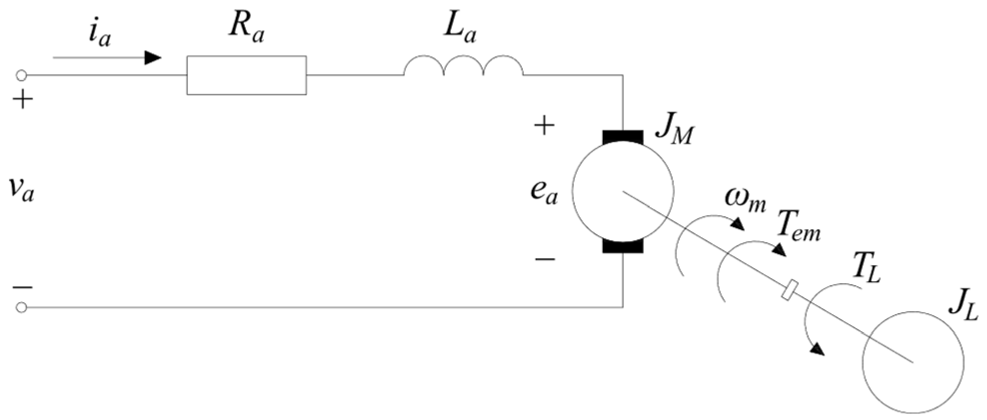
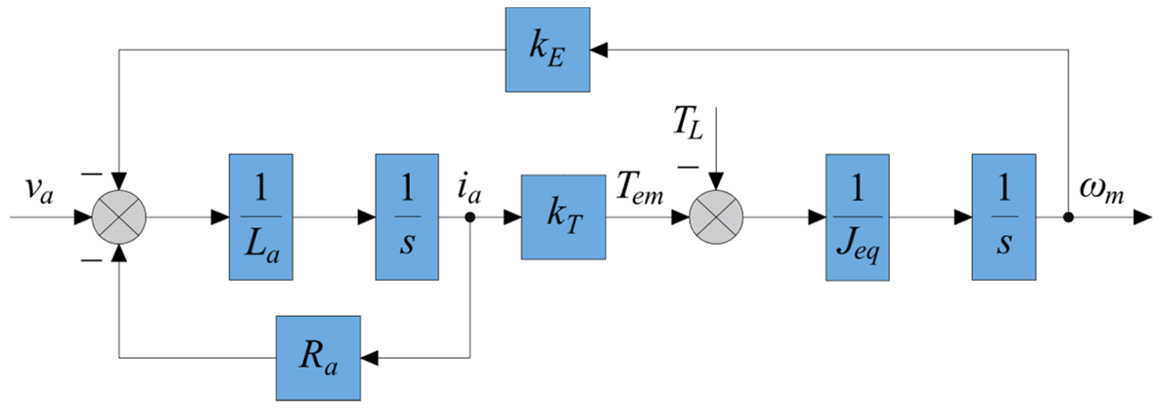
This section presents the non-model-based sensorless method used to estimate the speed of the brushed DC motor from the measured motor current. The purpose of employing the non-model-based method is to have a parameter-independent method which is accurate, simple to implement, and does not have large computational requirements. In this method, it is necessary to know the exact frequency of the current ripple to extract information about the rotor speed from the measured motor current. It is clear from Equation (11) that the frequency of the current ripple is proportional to the rotor speed and therefore changes in the frequency domain. This frequency can be extracted by the discrete bandpass filter, which is used for eliminating the DC component with frequency $f_{DC}$, the PWM component with frequency $f_{PWM}$, and the other spectral components from the motor current. A bandwidth of the bandpass filter has to be chosen appropriately to eliminate frequencies, which are not coupled to the rotor speed.

The first option is to use a wide bandwidth, with the bottom and top cut-off frequencies $f_B$ and $f_T$, respectively (Figure 8). The purpose of this approach is to cover an area of the ripple component for the lower rotational speed $n_{m_1}$ and the higher rotational speed $n_{m_2}$. However, this may lead to uncertainties in speed estimation because the ripple component coupled to the rotational speed is influenced by the other spectral components with smaller amplitude, as can be seen practically from the FFT in Figure 6. This approach can be performed either externally with the analogue bandpass filter or internally by the discrete bandpass filter.

The second option is to use a narrower bandwidth whose position is floating in the frequency domain according to the required rotor speed (Figure 9). Therefore, the ripple component at rotational speed $n_{m_1}$ or $n_{m_2}$ no longer contains most of the other spectral components, which are not corresponding to the rotor speed, and the speed can be estimated more accurately. This approach can be performed only by the discrete bandpass filter, which allows for appropriate bandwidth variation according to the rotor speed. The bandwidth variation is provided by means of the offline precalculated coefficients of the discrete bandpass filter. The coefficients can be calculated with the following MATLAB function:

$$\left[b, a\right]=\mathrm{butter}\left(n, W_n,f_{type}\right)$$

(13)

which returns the transfer function coefficients for the $f_{type}$ filter, for example, lowpass, highpass, bandpass, or bandstop. The resulting bandpass and bandstop designs are of order $2n$ with normalized cut-off frequency $W_n$. Solving Equation (13) for a given type of filter and cut-off frequency will produce five coefficients: $b_0$, $b_1$, $b_2$, $a_1$, $a_2$. These coefficients can be implemented into a microcontroller unit with the polynomial approximation or Look-up-table (LUT). In this paper, polynomial approximation was used, yielding lower computational requirements.

The output of the bandpass filter then provides a clean AC signal, which corresponds to the actual rotor speed. This signal is compared to a reference value to convert the ripples to pulses with a frequency equal to the frequency of the current ripple. The timer peripheral on a microcontroller unit is used to measure the length of each pulse, and the rotor speed can be estimated. The processing of the ripple current is performed by the microcontroller unit, thus without the use of any external components. The conversion of the measured motor current to the pulses is shown in Figure 10.

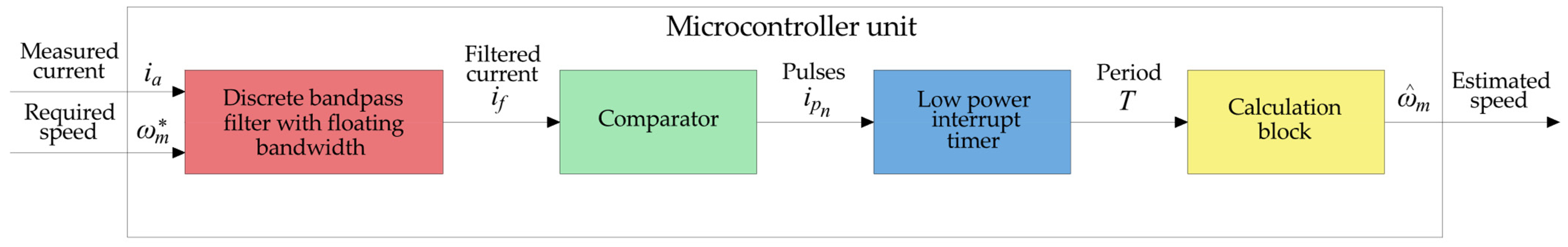
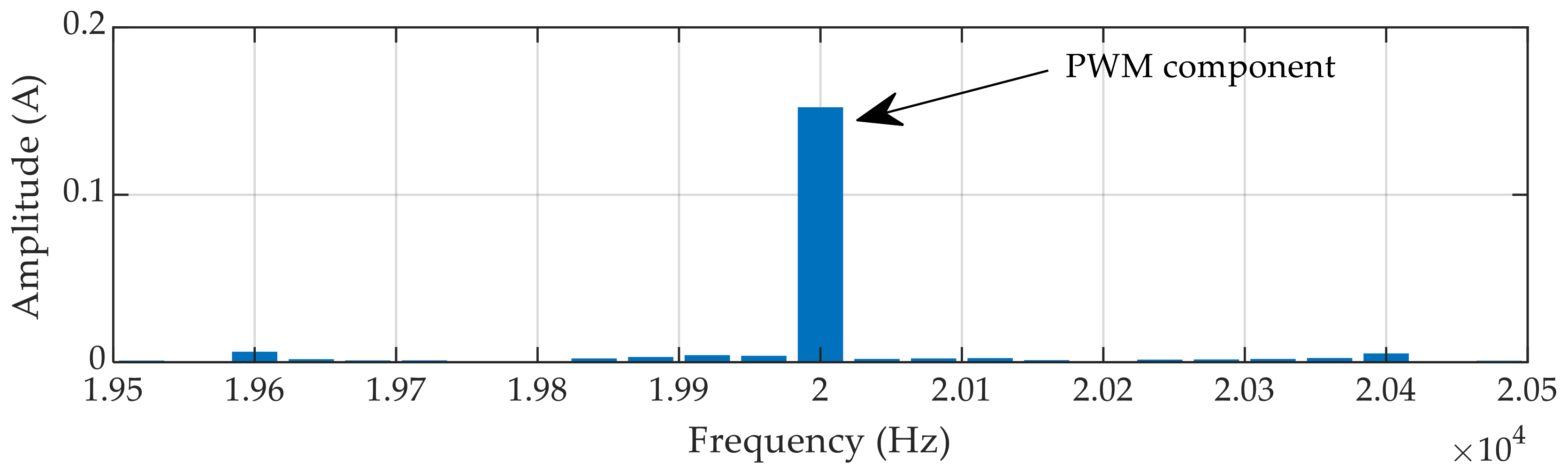
The block diagram of the current signal processing is presented in Figure 11 and the corresponding flowchart in Figure 12. The created pulses are used as an input to the timer peripheral (Low power interrupt timer—LPIT) to obtain information about the estimated speed. The variable $k_{\omega }$ in the flowchart represents the estimated speed scale constant. The data (Figure 10) were measured by a real-time debug monitor and the data visualization tool FreeMASTER. This tool has a limit for the number of recorded samples, so the high-frequency signal from PWM, as it is visible in Figure 5, is not presented in Figure 10.

4. Simulation Studies

In this section, the proposed non-model-based sensorless method will be simulated. The motor parameters which are mandatory to perform simulation tests were calculated based on the experimental procedures. These parameters are provided in

Table 2. Parameters of brushed DC motor.

Parameter	Symbol	Value
Nominal voltage	$V_{a_N}$	12 V
No load current	$I_o$	1.2 A
Armature resistance	$R_a$	0.697 Ω
Armature inductance	$L_a$	1.523 mH
Back-emf constant	$k_E$	0.0173 Vs/rad
Moment of inertia	$J_M$	1.970·10−6 kg· m2

. The parameters of a cascade control structure, which consists of PI controllers, will be also calculated in this section.

4.1. Current Loop

In order to obtain a transfer function for the electrical part of the DC motor, it is necessary to perform the Laplace transform of Equation (1) and express the armature current as follows:

$$i_a=\frac{v_a-k_E{\omega }_m}{\left(\frac{L_a}{R_a}s+1\right)R_a}=\frac{K_a{v}_a}{{\tau }_{a}s+1}-\frac{K_a{k}_E{\omega }_m}{{\tau }_{a}s+1}$$

(14)

where $K_a$ is the rotor gain and ${\tau }_a$ is the rotor time constant:

$$K_a=\frac{1}{R_a} {\tau }_a=\frac{L_a}{R_a}$$

(15)

By neglecting the second part of Equation (14), which is the influence of the back-emf, the transfer function for the electrical part of the DC motor in the Laplace domain is given as:

$$F_{RL}\left(s\right)=\frac{K_a}{{\tau }_{a}s+1}$$

(16)

This transfer function is a part of Figure 13, where a current loop including the PI controller is presented. The PI controller in the current loop is forcing to zero the error between the required armature current $i_a^{*}$ and the actual armature current $i_a$. The output of this controller, also known as a current controller, provides information about the required armature voltage $v_a^{*}$.

The transfer function of the current controller is given as:

$$F_{P{I}_i}\left(s\right)=\frac{K_{P_i}s+K_{I_i}}{s}$$

(17)

where $K_{P_i}$ is the proportional gain of the current controller and $K_{I_i}$ is the integral gain of the current controller. The open current loop transfer function is derived by the equation:

$$F_{o_i}\left(s\right)=\frac{K_{P_i}s+K_{I_i}}{s}\frac{K_a}{{\tau }_{a}s+1}=\frac{K_{P_i}\left(s{T}_{I_i}+1\right)}{T_{I_i}s}\frac{K_a}{{\tau }_{a}s+1}$$

(18)

where $T_{I_i}$ is the time constant of the current controller. According to the inverse dynamics method, the following condition is applied $T_{I_i}={\tau }_a$, which yields to the resulting open current loop transfer function:

$$F_{o_i}\left(s\right)=\frac{K_{P_i}\left(s{T}_{I_i}+1\right)}{T_{I_i}s}\frac{K_a}{{\tau }_{a}s+1}=\frac{K_{P_i}{K}_a}{T_{I_i}s}$$

(19)

By applying Mason’s rule, a closed current loop transfer function is derived as:

$$F_i\left(s\right)=\frac{F_{o_i}\left(s\right)}{1+F_{o_i}\left(s\right)}\frac{\frac{K_{P_i}{K}_a}{T_{I_i}s}}{1+\frac{K_{P_i}{K}_a}{T_{I_i}s}}=\frac{K_{P_i}{K}_a}{T_{I_i}s+K_{P_i}{K}_a}=\frac{1}{\frac{T_{I_i}}{K_{P_i}{K}_a}s+1}$$

(20)

The current loop will be replaced by 1st order transfer function with the time constant $T_{I_a}$, which is equal to:

$$T_{I_a}=\frac{T_{I_i}}{K_{P_i}{K}_a}$$

(21)

where $T_{I_a}$ is the time constant of the current loop. The proportional gain of the current controller is then derived from Equation (21):

$$K_{P_i}=\frac{T_{I_i}}{T_{I_a}{K}_a}$$

(22)

where $T_{I_a}$ can be expressed with respect to the settling time $T_{set}$ of the current loop:

$$T_{I_a}=\frac{T_{set}}{3}$$

(23)

The integral gain of the current controller can be calculated as:

$$K_{I_i}=\frac{K_{P_i}}{T_{I_i}}$$

(24)

The natural frequency of the current loop can be defined by Dodds’s formula:

$${\omega }_0=1.5\left(n+1\right)\frac{1}{T_{set}}$$

(25)

where $n$ is the order of the system. Considering the discrete domain, the expressions for controller gains will change as follows:

$$K_{P_i}\left(z\right)=K_{P_i}\left(s\right) K_{I_i}\left(z\right)=K_{I_i}\left(s\right)T_{s_i}$$

(26)

where $T_{s_i}$ is the sampling period of the current loop. The calculated parameters for the current loop can be found in

Table 3. Parameters of the current loop.

Parameter	Symbol	Value
Proportional gain	$K_{P_i}$	0.0914
Integral gain	$K_{I_i}$	41.820
Settling time	$T_{set}$	0.05 s
Order of the system	$n$	1
Natural frequency	${\omega }_0$	60 rad/s

.

In Figure 14, the comparison between the measured and simulated current is shown. The comparison was made for a step change from 0 A to 6 A with the settling time of the current loop equal to 0.05 s.

It is worth mentioning that the settling time for the current loop can be much smaller, approximately about 0.005 s, but for the proposed sensorless method, the bandwidth of the PI controller has to be limited to not affect the ripple in the measured current.

Figure 15 shows the Bode plot of the current loop, which expresses the magnitude and phase shift of the frequency response. The comparison between results from the simulation and measurement are presented. The dashed line in the figure shows the natural frequency of the current loop which is 60 rad/s.

4.2. Speed Loop

The parameters of the speed controller will be calculated according to the block diagram in Figure 16, where the current loop is replaced with the 1st order transfer function with the time constant $T_{I_a}$. The PI controller in the speed loop is forcing to zero the error between the required rotor speed ${\omega }_m^{*}$ and the actual rotor speed ${\omega }_m$. The output of this controller provides information about the required armature current $i_a^{*}$. The open speed loop transfer function can be written according to the block diagram in Figure 16:

$$F_{o_{\omega }}\left(s\right)=F_{P{I}_{\omega }}\left(s\right)F_i\left(s\right)k_T\frac{1}{J_{eq}s}=\frac{K_{P_{\omega }}\left(s{T}_{I_{\omega }}+1\right)}{T_{I_{\omega }}s}\frac{1}{T_{I_a}s+1}{k}_T\frac{1}{J_{eq}s}$$

(27)

By applying Mason’s rule, a transfer function of the closed speed loop is presented as:

$$F_{\omega }\left(s\right)=\frac{F_{o_{\omega }}\left(s\right)}{1+F_{o_{\omega }}\left(s\right)}=\frac{\frac{K_{P_{\omega }}\left(s{T}_{I_{\omega }}+1\right)}{T_{I_{\omega }}s}\frac{1}{T_{I_a}s+1}{k}_T\frac{1}{J_{eq}s}}{1+\frac{K_{P_{\omega }}\left(s{T}_{I_{\omega }}+1\right)}{T_{I_{\omega }}s}\frac{1}{T_{I_a}s+1}{k}_T\frac{1}{J_{eq}s}}$$

(28)

The resulting closed speed loop can be obtained by adjusting Equation (28) to the form:

$$F_{\omega }\left(s\right)=\frac{\frac{K_{P_{\omega }}{k}_T}{T_{I_{\omega }}{T}_{I_a}{J}_{eq}}\left(T_{I_{\omega }}s+1\right)}{s^3+s^2\frac{1}{T_{I_a}}+s\frac{K_{P_{\omega }}{k}_T}{T_{I_a}{J}_{eq}}+\frac{K_{P_{\omega }}{k}_T}{T_{I_{\omega }}{T}_{I_a}{J}_{eq}}}$$

(29)

However, the speed controller introduced a zero to the closed-loop transfer function for command changes, located at the numerator of Equation (29). This derivative characteristic of the loop increases the system overshoot, lowering the potential closed-loop bandwidth. Due to this, the zero of the speed controller must be compensated. This can be done by introducing a zero-cancellation block, which has the following transfer function:

$$F_{ZC}\left(s\right)=\frac{1}{T_{I_{\omega }}s+1}$$

(30)

The zero-cancellation block physically behaves as a low pass filter, smoothing the input command. It therefore allows for increasing of the loop gain, achieving a higher bandwidth. The speed loop transfer function with the zero-cancellation block in feed-forward is then:

$$F_{\omega }\left(s\right)=\frac{\frac{K_{P_{\omega }}{k}_T}{T_{I_{\omega }}{T}_{I_a}{J}_{eq}}}{s^3+s^2\frac{1}{T_{I_a}}+s\frac{K_{P_{\omega }}{k}_T}{T_{I_a}{J}_{eq}}+\frac{K_{P_{\omega }}{k}_T}{T_{I_{\omega }}{T}_{I_a}{J}_{eq}}}$$

(31)

The block diagram of the speed loop with the zero-cancellation is shown in Figure 17.

Having the closed loop with a canceled zero (Equation (31)), the parameters of the speed controller can be calculated by exploiting a pole placement method. A pole placement method is an approach of a feedback control system theory to place the closed-loop poles of a plant in predetermined locations. The pole placement method applied to the closed-loop system leads to desired controlled system behavior. The parameters are designed by comparing the characteristic polynomial with that of a standard third-order system, as follows:

$$s^3+s^2\frac{1}{T_{I_a}}+s\frac{K_{P_{\omega }}{k}_T}{T_{I_a}{J}_{eq}}+\frac{K_{P_{\omega }}{k}_T}{T_{I_{\omega }}{T}_{I_a}{J}_{eq}}=s^3+s^2\left(2\xi {\omega }_0+{\omega }_0\right)+s\left(2\xi {\omega }_0^2+{\omega }_0^2\right)+{\omega }_0^3$$

(32)

where $\xi$ is the loop attenuation. The settling time of the speed loop can be defined by Dodds’s formula:

$${\omega }_0=1.5\left(n+1\right)\frac{1}{T_{set}}$$

(33)

The proportional gain of the PI controller can be therefore calculated by the following equation:

$$K_{P_{\omega }}=\frac{\left(2\xi {\omega }_0^2+{\omega }_0^2\right)T_{I_a}{J}_{eq}}{k_T}$$

(34)

and the integral gain:

$$K_{I_{\omega }}=\frac{{\omega }_0^3{T}_{I_a}{J}_{eq}}{k_T}$$

(35)

where $T_{I_a}$ is given from Equation (32):

$$T_{I_a}=\frac{1}{\left(2\xi {\omega }_0+{\omega }_0\right)}$$

(36)

Considering the discrete domain, the expressions will change as follows:

$$K_{P_{\omega }}\left(z\right)=K_{P_{\omega }}\left(s\right)\hspace{1em}\hspace{1em}\hspace{1em}{K}_{I_{\omega }}\left(z\right)=K_{I_{\omega }}\left(s\right)T_{s_{\omega }}$$

(37)

where $T_{s_{\omega }}$ is the sampling period of the speed loop. The parameters of the current controller will be recalculated concerning the time constant obtained from Equation (36). The calculated parameters for the speed loop can be found in

Table 4. Parameters of the speed loop.

Parameter	Symbol	Value
Proportional gain of the speed controller	$K_{P_{\omega }}$	0.0017
Integral gain of the speed controller	$K_{I_{\omega }}$	0.0085
Proportional gain of the current controller	$K_{P_i}$	0.0685
Integral gain of the current controller	$K_{I_i}$	31.365
Settling time	$T_{set}$	0.4 s
Order of the system	$n$	3
Natural frequency of the speed controller	${\omega }_0$	15 rad/s
Loop attenuation	$\xi$	1

.

In Figure 18, the comparison between the measured and simulated speed is shown. The comparison was made for a speed step change from 0 rpm to 3000 rpm with the settling time of the speed loop equal to 0.4 s.

It should be noticed that the current loop is faster than the speed loop. This can be done because, in most cases, the electrical time constant of the motor is much smaller than the mechanical time constant of the motor and so the small electrical time constant requires the current control loop to run at a higher sampling frequency. On the contrary, the speed loop regarding the higher time constant can run in a slower control loop with a lower sampling frequency. Such an approach provides enough time to control the current between two speed samples.

Figure 19 shows the Bode plot of the speed loop, where the comparison between the results from simulation and measurement are presented. The dashed line in the figure shows the natural frequency of the speed loop, which is 15 rad/s.

4.3. Sensorless Speed Estimation

Figure 20 shows the complete block diagram of the proposed sensorless control applied to the simulation.

The block diagram includes three main parts where the first part is a control structure, which is composed of the zero-cancellation block, the speed controller, and the current controller. The second part is the proposed sensorless method, which was introduced in Section 3 and represented with a block diagram in Figure 11. The last part is the dynamic model of the DC motor is a second-order linear system. The more detail-enriched model considering nonlinearity effects, such as the cogging torque and streback effect, is presented in [14].

As was already mentioned, the dynamic model of DC motor, as illustrated in Figure 2, does not include the effect of commutation. One of the solutions for how to include this effect and perform the simulation is to inject a periodic signal with the exact frequency of current ripple into the motor current. The frequency of this signal will change with the rotor position. This effect is included in the block diagram with a block named ripple. After this injection, the simulation of the proposed sensorless method can be performed according to the block diagram.

Figure 21 shows the results obtained from the simulation model for a speed step change from 0 rpm to 3000 rpm. There is a comparison between the required rotor speed ${\omega }_m^{*}$, actual rotor speed ${\omega }_m$ and estimated rotor speed ${\widehat{\omega }}_m$. The simulation results show a good match between the speed obtained from the dynamic model and the estimated speed from the proposed sensorless method. The parameters of the speed and current controller were set according to Table 4.

5. Experimental Results

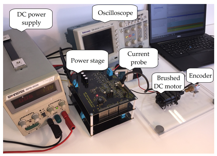
The tests were performed on the 3-phase low voltage power stage controlled as a full bridge DC/DC converter with apparent power up to 420 VA. The nominal apparent power and nominal current of the power stage are 300 VA and 20 A, respectively. The power stage was made by the author for the dual-motor control applications. However, as Table 2 yields, the no-load current of the experimental motor is 1.2 A. It has to be pointed out that the apparent power of 300 VA is just the nominal value of the power stage, but not the nominal power of the experimental system. The brushed DC motor with a stationary magnetic field generated by permanent magnets was used for the experiments. The motor parameters are given in Table 2. As the microcontroller unit, a S32K144EVB from NXP Semiconductors was used, which is a low-cost evaluation and development board for general purpose automotive applications. The S32K144EVB is based on the 32-bit Arm^® Cortex^®-M4F S32K14 and offers a standard-based form factor compatible with the Arduino^® UNO pin layout, providing a broad range of expansion board options for quick application prototyping and demonstration. The communication between S32K144EVB and PC is provided by serial and debug adapter OpenSDA. It secures a bridge between PC and the embedded target processor, which can be used for debugging, flash programming and serial communication. The control algorithm was created in the S32 Design Studio for Arm^®, which is a complimentary Integrated Development Environment (IDE) for automotive and ultra-reliable Arm-based microcontrollers that enable editing, compiling, and debugging of designs. The current was measured on the low voltage power stage by the 5 mΩ shunt resistor with the sampling frequency equal to 20 kHz. An incremental encoder with 2048 pulses per one rotation was attached to the motor shaft to provide reliable information about the actual rotor speed. The oscilloscope Tektronix TDS 2022B was used to provide motor current figures with a high number of samples. The speed data was measured by a real-time debug monitor and data visualization tool FreeMASTER. The photo of an experimental setup is shown in Figure 22 and Figure 23.

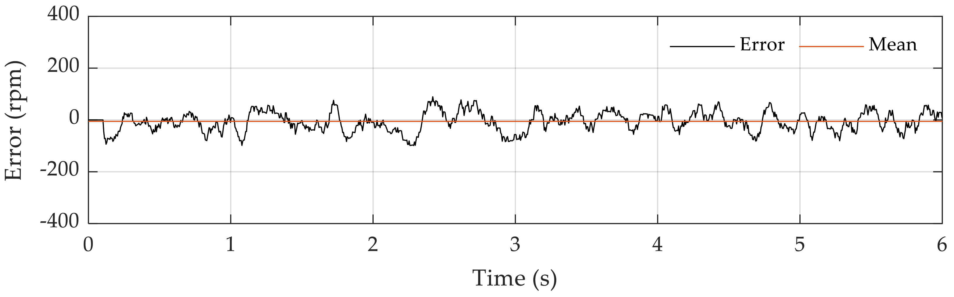
Figure 24 shows the comparison between the actual and estimated rotor speed for a speed step from 0 rpm to 3000 rpm, and Figure 25 shows the error between these speeds.

A motor start-up was provided in the open loop. At the speed of 700 rpm, the estimated speed was set as a feedback value to the speed controller. This method is not suitable for speeds below 700 rpm, which is the main limitation of this method. The reason is that below this speed, the frequency of the current ripple is small enough. Therefore, the control algorithm does not have enough information about the rotor speed from the measured current to provide reliable speed control. It can be compared to a sensor having a low number of references about the rotor speed per one rotation. The value of the threshold speed for controlling the motor speed appropriately depends on the motor construction parameters from Equation (9). For example, motors with a larger number of commutator segments provide enough information about the rotor speed also at the low speeds. That is due to the higher frequency of the current ripple. However, as was already mentioned in Section 2, a larger number of commutator segments will lead to a smaller amplitude of the current ripple, which may lead to more difficult signal processing.

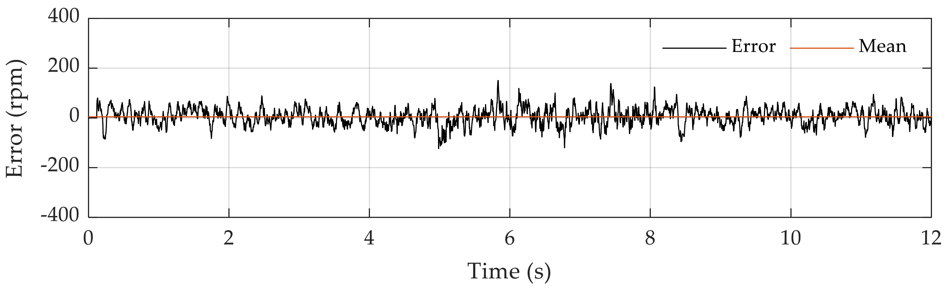
Figure 26 shows the comparison between the same speeds, but for stepped changes of required speed from 0 rpm to 6000 rpm.

As in the previous case, the estimated speed was set as a feedback value at 700 rpm. This test was performed to show the accuracy of the proposed method for a wide speed range. The error between the actual and estimated speed is shown in Figure 27, where the mean value of the error is about 1.907 rpm, which is 0.032%. According to the results obtained from Figure 26 and Figure 27, it can be said that this method works accurately in a tested speed range, which was from 700 rpm to speed 6000 rpm. The tested range presents 88.333% of the whole speed range. It is worth mentioning that this method has the potential to work also for very high-speed DC motors. At very high speeds, the number of ripples per one rotation is adequate to control the motor speed.

One can observe that the ripple of the estimated speed is increasing with a higher rotational speed. This phenomenon is a result of the DC motor nonlinearities. In the higher speeds, there are frequencies, which are very close to the frequency of the current ripple related to the commutation process. As a result, the output of the discrete band-pass filter is not a clean AC signal. According to this fact, pulses created by the comparator will have different lengths. These lengths are measured by the timer, leading to the presence of the ripple in the estimated speed. However, it is possible to reduce the ripple in the estimated speed by choosing the smaller bandwidth of the proposed filter. Nevertheless, it is not a necessary condition because the ripple is not presented in the actual rotor speed, measured by the mechanical sensor, due to the PI controllers located in the cascade control structure. The PI controller acts as a filter, which is eliminating the ripple from the feedback estimated speed.

Figure 28 and Figure 29 reveal that the proposed sensorless method also works correctly under load conditions. During the motor operation, a load of 0.002 Nm was applied to the rotor shaft. It shows the robustness of the proposed sensorless method against step change of the load torque.

The proposed sensorless method works even better under load conditions due to the current ripple resolvability (Figure 30). This figure shows the motor current at three different load conditions. It can be seen from the figure that with the higher applied load, not just the amplitude of the DC component is increased but also the amplitude of the presented AC component due to the commutation process.

Most of the motors are used in applications where the load is coupled to the rotor shaft or its value changes during motor operation. According to this fact, the proposed sensorless method is suitable for such applications. The experimental motor is primarily used for window lifter applications in the automotive sector, where the Hall effect sensor is used as a mechanical sensor. The applications where the proposed sensorless approach would see a real benefit in the case of speed control are applications such as pumps, fans, and so on. The position control with the proposed sensorless approach could expand an application area to the automotive industry in applications such as window lifters, seat positioning, sunroofs, and so on.

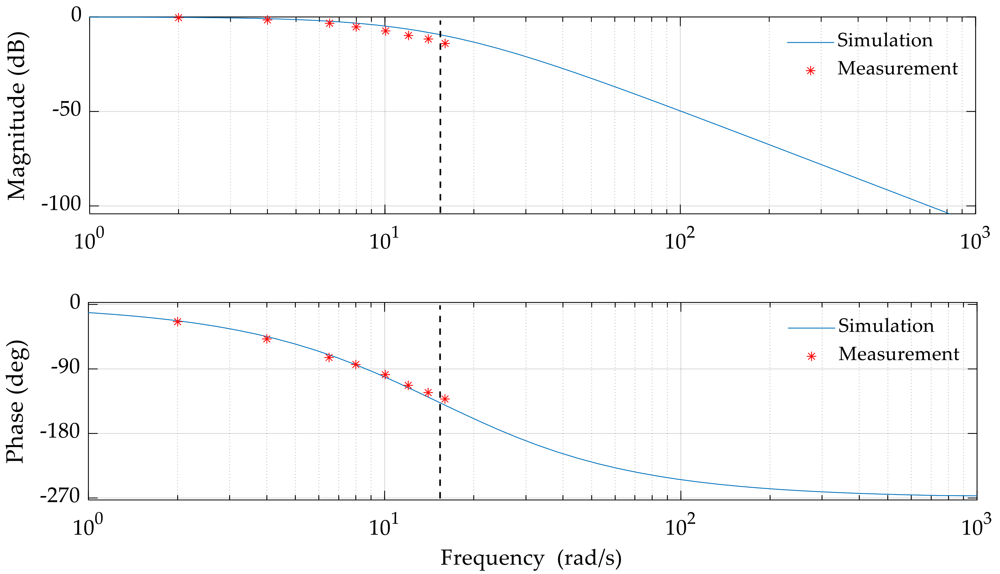
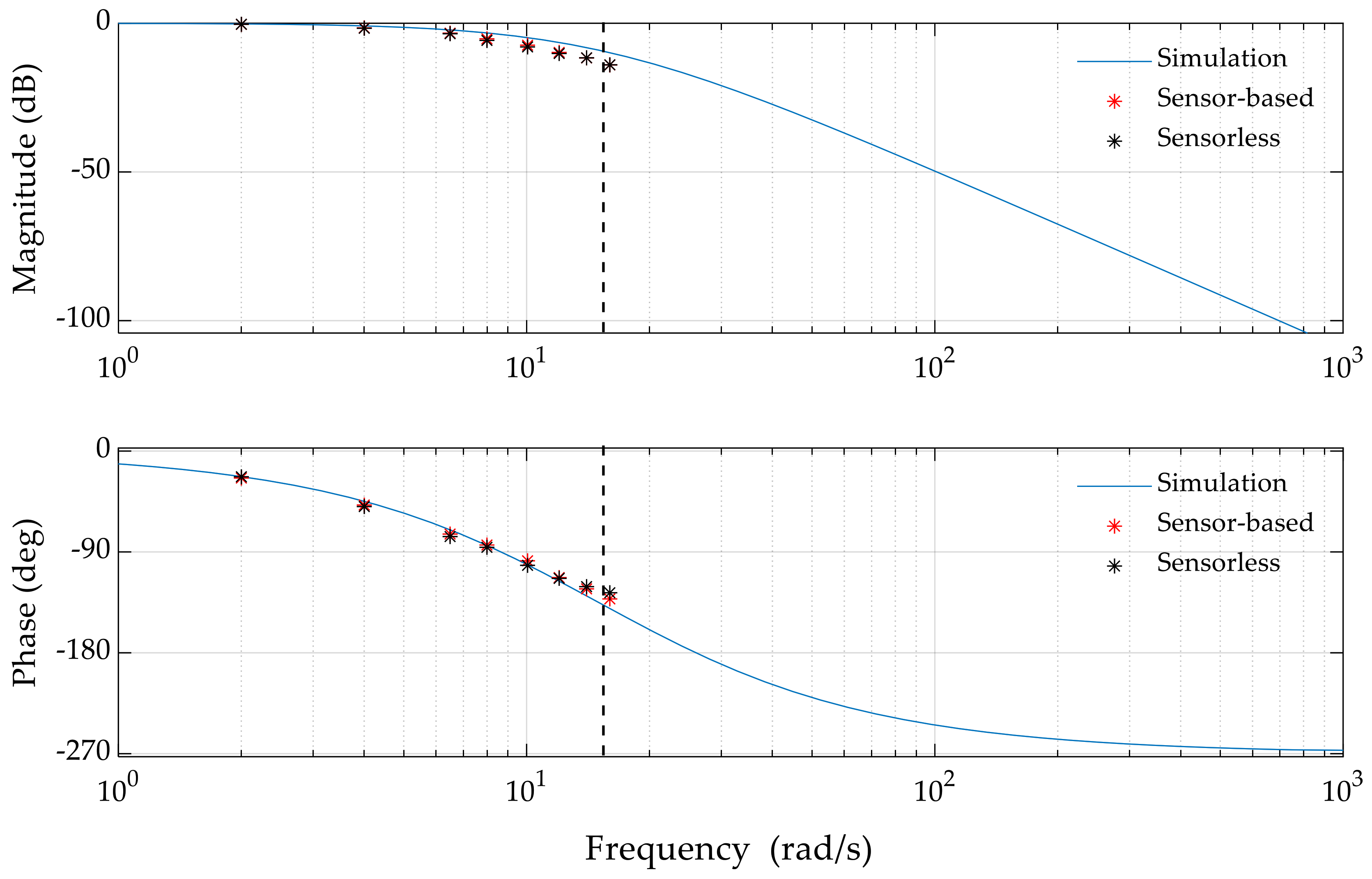
Figure 31 shows the Bode plot of the speed loop for sensor-based and sensorless control with a very good match. The results were compared to the ideal transfer function from the simulation. The dashed line in the figure shows the natural frequency of the speed loop, which is 15 rad/s in both cases.

6. Conclusions

Signal processing of the brushed DC motor current was developed and presented in this paper. This method used the ripple component of the brushed DC motor current to estimate the rotor speed. The discrete bandpass filter with the floating bandwidth, discrete comparator, and timer peripheral on the microcontroller unit were used to extract information about the rotor speed from the motor current. The experimental verification of the proposed sensorless method was performed and compared to the simulation. The accuracy of the proposed sensorless method was investigated, where the error between the actual speed obtained from the mechanical sensor and the estimated speed obtained from the proposed sensorless method was about 0.032%. However, this sensorless method also has some limits. The first limit lies in the control dynamics, where the bandwidth of the current controller had to be limited to not affect the ripple in the motor current. The second limit lies in the incapability of the proposed structure to control the rotor speed at low speeds. The threshold speed depends on the motor construction. It is specifically on the number of commutator segments, their parity, and the number of pole pairs. The value of the threshold speed for the motor used in this study was approximately 700 rpm. Nevertheless, this sensorless method works accurately and precisely in a wide speed range, which is from 700 rpm to 6000 rpm. This range presents 88.333% of the whole speed range. Therefore, this sensorless method can be used as a redundant solution in case of a sudden mechanical sensor failure in DC drives, where the operational speed is higher and the system requires accurate and reliable information about the rotor speed.

References

1. Bowes, S.R.; Sevinc, A.; Holliday, D. New natural observer applied to speed-sensorless DC servo and Induction motors. IEEE Trans. Ind. Electron. 2004, 51, 1025–1032. [Google Scholar] [CrossRef]
2. Weerasooriya, S.; El-Sharkawi, M.A. Identification and control of a DC motor using back-propagation neural networks. IEEE Trans. Energy Convers. 1991, 6, 663–669. [Google Scholar] [CrossRef]
3. Razi, R.; Monfared, M. Simple control scheme for single-phase uninterruptible power supply inverters with Kalman filter-based estimation of the output voltage. IET Power Electron. 2015, 8, 1817–1824. [Google Scholar] [CrossRef] [Green Version]
4. Castaneda, E.C.; Loukianov, G.A.; Sanchez, N.E.; Castillo-Toledo, B. Discrete-Time Neural Sliding-Mode Block Control for a DC Motor with Controlled Flux. IEEE Trans. Ind. Electron. 2012, 59, 1194–1207. [Google Scholar] [CrossRef]
5. Scott, J.; McLeish, J.; Round, H. Speed Control with Low Armature Loss for Very Small Sensorless Brushed DC Motors. IEEE Trans. Electron. 2009, 56, 1223–1229. [Google Scholar] [CrossRef] [Green Version]
6. Ramli, R.M.; Mikami, N.; Takahashi, H. Adaptive filters for rotational speed estimation of a sensorless DC motor with brushes. In Proceedings of the 10th International Conference on Information Science, Signal Processing and their Applications (ISSPA 2010), Kuala Lumpur, Malaysia, 10–13 May 2010. [Google Scholar]
7. Vazquez-Sanchez, E.; Gomez-Gil, J.; Gamazo-Real, J.C. A New Method for Sensorless Estimation of the Speed and Position in Brushed DC Motors Using Support Vector Machines. IEEE Trans. Ind. Electron. 2012, 59, 1397–1408. [Google Scholar] [CrossRef]
8. Radcliffe, P.; Kumar, D. Sensorless speed measurement for brushed DC motors. IET Power Electron. 2015, 8, 2223–2228. [Google Scholar] [CrossRef]
9. Vazquez-Sanchez, E.; Sottile, J.; Gomez-Gil, J. A Novel Method for Sensorless Speed Detection of Brushed DC Motors. Appl. Sci. 2016, 7, 14. [Google Scholar] [CrossRef] [Green Version]
10. Texas Instruments: Automotive Brushed-Motor Ripple Counter Reference Design for Sensorless Position Measurement. 2018. Available online: https://www.ti.com/lit/ug/tidud30a/tidud30a.pdf (accessed on 14 June 2018).
11. Microchip Technology Inc: Sensorless Position Control of Brushed DC Motor Using Ripple Counting Technique. 2019. Available online: http://ww1.microchip.com/downloads/en/AppNotes/Sensorless-Position-Control-of-Brushed-DC-Motor-Using-Ripple-Counting-Technique-00003049A.pdf (accessed on 17 June 2019).
12. Vidlak, M.; Makys, P.; Stano, M. Comparison between model based and non-model based sensorless methods of brushed DC motor. Transp. Res. Procedia 2021, 55, 911–918. [Google Scholar] [CrossRef]
13. Yuan, B.; Hu, Z.; Zhou, Z. Expression of Sensorless Speed Estimation in Direct Current Motor with Simplex Lap Winding. In Proceedings of the International Conference on Mechatronics and Automation, Harbin, China, 5–8 August 2007. [Google Scholar]
14. Dini, P.; Saponara, S. Design of Adaptive Controller Exploiting Learning Concepts Applied to a BLDC-Based Drive System. Energies 2020, 13, 2512. [Google Scholar] [CrossRef]
Figure 1. Equivalent circuit of DC motor.
Energies 14 05359 g001
Figure 2. Block diagram of DC motor.
Energies 14 05359 g002
Figure 3. Commutation process of a DC machine with four commutator segments and one pole pair at: (a) θ m = 0 ; (b) θ m = 45 ° ; (c) θ m = 90 ° .
Energies 14 05359 g003
Figure 4. Commutation process of a DC machine with three commutator segments and one pole pair at: (a) θ m = 0 ; (b) θ m = 30 ° ; (c) θ m = 60 ° .
Energies 14 05359 g004
Figure 5. Brushed DC motor current—comparison.
Energies 14 05359 g005
Figure 6. Brushed DC motor current in the frequency domain—DC component and ripple component.
Energies 14 05359 g006
Figure 7. Brushed DC motor current in the frequency domain—PWM component.
Energies 14 05359 g007
Figure 8. Discrete bandpass filter with fixed bandwidth: (a) the lower rotational speed; (b) the higher rotational speed.
Energies 14 05359 g008
Figure 9. Discrete bandpass filter with the floating bandwidth: (a) the lower rotational speed; (b) the higher rotational speed.
Energies 14 05359 g009
Figure 10. Signal processing of the measured motor current with a rotational speed of 3000 rpm.
Energies 14 05359 g010
Figure 11. Block diagram of the current signal processing.
Energies 14 05359 g011
Figure 12. Flowchart of the current signal processing.
Energies 14 05359 g012
Figure 13. Block diagram of the current loop.
Energies 14 05359 g013
Figure 14. Comparison between the measured and simulated current, with a required current of 6 A.
Energies 14 05359 g014
Figure 15. Bode plot of the current loop frequency response.
Energies 14 05359 g015
Figure 16. Block diagram of the speed loop.
Energies 14 05359 g016
Figure 17. Block diagram of the speed loop with the zero cancellation.
Energies 14 05359 g017
Figure 18. Comparison between the measured and simulated speed, with a required speed of 3000 rpm.
Energies 14 05359 g018
Figure 19. Bode plot of the speed loop frequency response.
Energies 14 05359 g019
Figure 20. Block diagram of the proposed sensorless control.
Energies 14 05359 g020
Figure 21. Comparison between the speeds obtained from the simulation model, with a required speed of 3000 rpm.
Energies 14 05359 g021
Figure 22. Photo of the experimental setup.
Energies 14 05359 g022
Figure 23. Photo of the experimental setup.
Energies 14 05359 g023
Figure 24. Comparison between the speeds obtained from the measurement and simulation, with a required speed of 3000 rpm.
Energies 14 05359 g024
Figure 25. The error between the actual and estimated speeds obtained from the measurement, with a required speed of 3000 rpm.
Energies 14 05359 g025
Figure 26. Comparison between the speeds obtained from the measurement and simulation, with stepped changes of required speed from 0 rpm to 6000 rpm.
Energies 14 05359 g026
Figure 27. The error between the actual and estimated speeds obtained from the measurement, with stepped changes of required speed from 0 rpm to 6000 rpm.
Energies 14 05359 g027
Figure 28. Comparison between the speeds obtained from the measurement and simulation, with a required speed of 3000 rpm and applied load of 0.002 Nm during motor operation.
Energies 14 05359 g028
Figure 29. The error between the actual and estimated speeds obtained from the measurement, with a required speed of 3000 rpm and applied load of 0.002 Nm during motor operation.
Energies 14 05359 g029
Figure 30. The brushed DC motor current at three different load conditions with a rotational speed of 3000 rpm.
Energies 14 05359 g030
Figure 31. Bode plot of the speed loop frequency response for sensor-based and sensorless.
Energies 14 05359 g031