Prospects for the Application of Wavelet Analysis to the Results of Thermal Conductivity Express Control of Thermal Insulation Materials

Abstract

This article discusses an express control method that allows in situ measurements of the thermal conductivity of insulation materials. Three samples of the most common thermal insulation materials, such as polyurethane, extruded polystyrene, and expanded polystyrene, were studied. Additionally, optical and organic glasses were investigated as materials with a stable value of thermal conductivity. For the measurement of thermal conductivity, the express control device, which implements the differential method of local heat influence, was used. The case studies were focused on the reduction of fluctuations of the measured signals caused by different influencing factors using wavelet transform. The application of wavelet transform for data processing decreased the thermal conductivity measurement’s relative error for organic glass SOL and optical glasses TF-1 and LK-5. The application of wavelet transform thermal conductivity measurement data for polyurethane, extruded polystyrene, and expanded polystyrene allowed to reduce twice the duration of express control while maintaining the same level of measurement error. The results of the investigation could be used to increase the accuracy in express control of the thermal conductivity of insulation materials by improving the data processing. This approach could be implemented in software and does not require a change in the design of the measuring equipment or the use of additional tools.

1. Introduction

The need for economical treatment of energy consumption and energy savings has caused an increase in the demand for new insulation materials. These materials are used to reduce the heat losses from construction, utilities, heat, aerospace, etc. One of the main indicators of the quality of thermal insulation materials is the coefficient of thermal conductivity.

The methods of measuring thermal conductivity are usually divided into steady-state condition methods and transient condition methods [1,2,3,4].

Steady-state methods are based on Fourier’s law. Thermal conductivity in these methods is determined under steady-state heat flux passing through the sample by measuring the temperature difference in the case of guarded hot plates [1] and the heat flux in the case of heat flow meter apparatus [2,3]. These methods usually require relatively large samples, which allow studying porous materials and composites [3,4,5]. The disadvantages of steady-state methods are parasitic heat losses and contact resistance [6,7,8]. Experiments usually last from 3 to 8 h and the measurement error is 2–5% [1,2].

Transient methods assume that heat is supplied to the sample by impulse or periodically, resulting in periodic or transient temperature changes in the sample, respectively [3,9]. Most methods are based on indirect measurements of thermal diffusivity, which is an indicator of the rate of heat transfer throughout a material and is related to density and specific heat capacity. The most widespread transient methods are the transient plane source, transient hot wire, laser flash apparatus, modulated DSC, 3ω, and thermocouple methods [3,4,9]. The duration of the experiments for transient methods varies from a few seconds to a few minutes, but additional measurements and recalculations, in this case, can substantially increase the measurement error.

The main factors influencing the thermal conductivity of thermal insulation materials are temperature, moisture content, and bulk density [10,11]. During the storage and transportation of materials, the effect of these factors is especially tangible. This is why it is recommended to measure the thermal conductivity not only under laboratory conditions but also in situ, for example, the input quality control at a construction site. In this case, it is practical to use express methods for the control quality of thermal insulation materials.

Another important factor influencing thermal conductivity is the sample preparation for measurements. For all steady-state methods and some transient methods, the samples should be of a specific size and should have two parallel plane surfaces. This reduces their applicability to express tests of thermal conductivity.

In our previous works, a portable device for the express control of thermal conductivity measurements based on the method of local heat influence was described [12]. This device has advantages, such as acceptable measurement error and sufficiency of preparation of only one side of the samples. Moreover, the device allows one to measure porous materials with a pore diameter of 3 mm and materials with included particles size of up to 3 mm.

However, this device completely excludes influencing factors such as weather conditions, and changes in the thermophysical characteristics of materials that are sensitive to them is impossible. This leads to an increase in the fluctuations of the measured parameters during the experiment, i.e., an increase in the noise of the measured signals on the time scale could be observed. A well-known method for reducing this noise is wavelet transform.

There are many applications of wavelet analysis for measurement data processing. During data analysis, different wavelets can be used, e.g., Coiflets wavelets of the order of 1 [13], Daubechies wavelets of the order of 4 [14,15], or biorthogonal wavelets of the order of 3.1 [16]. As a result of data processing, the measurement accuracy [16] can be improved and data dimensionality reduced, which can then improve the learning ability of the neural network [17]. Wavelet transformation has been successfully used to assess the influence of the uncertainty of the input data for monitoring thermal parameters [18] and for the time scale representation of heat load time series [19]. In [20], wavelet transform was used for the analysis of the parameters of glass. Thus, wavelet transform can be used for the analysis of building materials. Based on all of this, we put forward a hypothesis about the possibility of the application of wavelet analysis to the results of thermal conductivity express control of thermal insulation materials.

This work aimed to improve the process of determining the thermal conductivity in the express control of materials with low thermal conductivity in terms of reducing the experiment duration and increasing the accuracy of the obtained results due to the use of the wavelet analysis for data processing.

The main novelty of this work lays in reducing the experiment duration and, at the same time, retaining the accuracy of the thermal conductivity measurement of insulation materials in manufacturing production, as well as during input quality control at the construction site, through the use of wavelet transform in the data processing. The results presented in this paper demonstrate the possibility of the operational control of the thermal conductivity of insulation materials with an accuracy that is not inferior to laboratory research methods.

2. Materials and Methods

2.1. Studied Specimens

The most widespread modern thermal insulation materials were investigated in the work. For the experimental studies, samples of materials were chosen with thermal conductivity values representing the range characteristic of thermal insulation and building materials, i.e., from 0.02 to 1.5 W/(m∙K). In the measurement range from 0.2 to 1.4 W/(m∙K), the samples with well-studied thermal conductivity made of organic and optical glass were used. Low-conductivity materials in the range of values less than 0.2 W/(m∙K), whose thermal conductivities are known from the results of previous studies, were used [2,21].

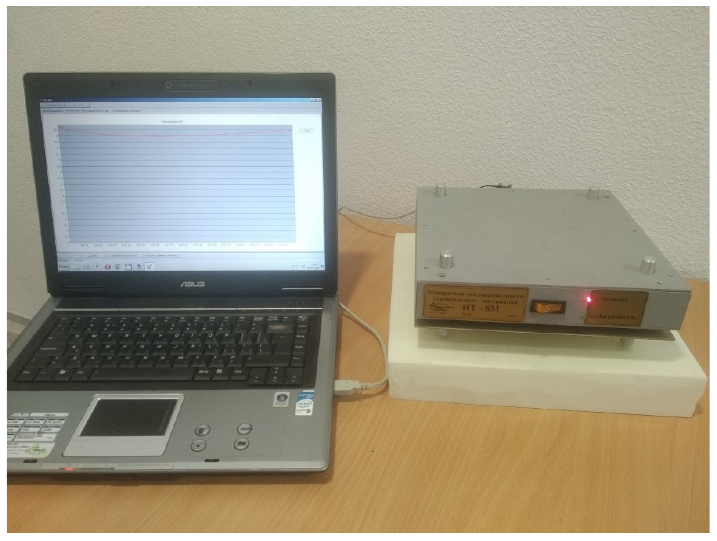
2.2. Experimental Equipment and Methods

For studying the thermal conductivity coefficient of thermal insulation materials, a portable device [12] for express control of thermal conductivity was used (Figure 1).

The main technical characteristics of the portable device for the express control of thermal conductivity are given in

Table 1. Technical specifications of the device for thermal conductivity measurement.

Parameter	Values or Value Range
The range of measured values of thermal conductivity	0.03 … 1.5 (W/(m∙K))
The operating temperature of the sample	25 ± 5 (°C)
Relative error	±8 (%)
Duration of the measurements	30 (min)

.

In this device, the coefficient of thermal conductivity is determined by the differential method of local heat influence. According to the differential method, the device is equipped with measuring probes with identical sensors of heat flux and temperature. One of them additionally contains a built-in electric heater, which is designed to create a thermal effect on the sample surface. The method of local heat influence is based on applying a heat flux of constant density to the sample surface through a probe with a heater, while the second probe remains undisturbed by the thermal effect area. In a steady thermal state, the coefficient of thermal conductivity can be found from the measurements of the heat flux difference and of the temperature difference between the heat zone and the sample surface, where the heat influence is absent, that is, according to the readings of these measuring probes [12]:

$$\lambda =K\frac{\Delta q}{\Delta T}=K\frac{q_0-q}{T_0-T},$$

(1)

where

• K—the calibration characteristic of the device (m);
• q₀, q—the measured values of heat flux in the undisturbed zone and the area of local heat, respectively (W/m²);
• T₀, T—the measured temperature values in the area of local heat in the undisturbed zone and the area of local heat, respectively (K).

The procedure of thermal conductivity determination using the portable device is as follows. The device is placed on a flat surface of the test material sample, connected to a computer with the appropriate software (Figure 1). The steady state of the system is established after 20–25 min. The onset of a steady state is determined by the operator from the visualized data displayed by the program. After establishing the stationary mode, the measurement mode starts, which lasts 5 min. The measurement result is the average value of the thermal conductivity calculated from the data set generated in the measurement mode.

The measurements and processing of the signals of heat flux and temperature primary sensors are automated. As heat flux sensors are based on the auxiliary wall principle [22], they are calibrated according to [23]. As a temperature sensor, the L differential thermocouple type is used. For registration of signals of the temperature and heat flux sensors, the 8-channel 16-bit ADC with a 10 Hz conversion rate is used. Afterward, the signals in digital form are transmitted through industrial interface RS-485 to a computer, where a software package registers and processes the measurement information. The values of the required thermal conductivity, as well as the temperature of the sample, are displayed in a computer program.

The recording of measurement information begins 25 min after the start of the experiment and lasts for 5 min. Processing of the recorded measuring information according to the standard procedure is carried out by the method of signal averaging:

$$\overline{\lambda }=\frac{1}{N}{\displaystyle \sum }_{i=1}^N{\lambda }_i,$$

(2)

where N is the number of measurements, N ≥ 10.

To compare the measurement results of the express control of the thermal conductivity coefficient of thermal insulation materials, a precision information-measuring system was used [21]. The information-measuring system’s principle of operation is determined by the standard symmetric measuring cell structure [2] using two identical thermoelectric heat flux meters. It creates a constant temperature difference between the working surfaces of the studied material flat sample and, accordingly, a uniform heat flow through the sample in directional perpendicular to its working surfaces. Thermal conductivity is calculated using the results of measuring the temperature difference between the working, upper heated, and lower cooled sample surfaces, the density of the heat flux passing through them in the steady state, and the thickness of the samples.

The technical characteristics of the heat flow meter apparatus [21] are

• Thermal conductivity coefficient measurements range from 0.02 to 3.0 (W/(m∙K));
• Main relative error of ±3%;
• Operating temperature ranges from −40 to +180 (°C);
• Sample size of 300 × 300 × (10…120) (mm).

2.3. Methods of Data Processing

The wavelet transform method was selected to analyze the thermal conductivity of materials in the range of 0.2–1.4 W/(m∙K).

The final result of the thermal conductivity value is obtained by recalculating the measured values of q and T by dependence (1). As this calculation is performed programmatically according to the current measurement data, which are recorded with a time step of 1 s, it is possible to consider the values of thermal conductivity thus obtained as a discrete signal. For the analysis of such signals, we can use wavelet transform to investigate the possibilities of improving the measurement results. We used wavelet analysis for additional processing of the express control data of the thermal conductivity of thermal insulation materials.

Wavelet analysis is used for the decomposition, reconstruction, and denoising reduction of time series. Discrete wavelet transform is based on wavelet coefficients, which are scalar products of the signal f(t) and the mother wavelet ψ_mn. Discrete inverse transform is defined by the following relationship [24]:

$$f\left(t\right)={\displaystyle \sum }_{m,n}\left(f,{\psi }_{mn}\right){\psi }_{mn}={\displaystyle \sum }_m{\displaystyle \sum }_n{d}_m\left[n\right]{\psi }_{mn},$$

(3)

where the wavelet coefficients d_m[n](f,ψ_mn) define the common features of the signal f(t) and the wavelet. The parameter m allows one to determine the scale level, and the parameter n enables signal location in time when signal f(t) should be analyzed.

Multiresolution analysis of the signal is based on discrete wavelet transform and can be defined by the following equation [24]:

$$f\left(t\right)={\displaystyle \sum }_{j=-\infty }^J{\displaystyle \sum }_{n\in Z}{d}_j\left[n\right]+{\displaystyle \sum }_{n\in Z}{a}_J\left[n\right]{\phi }_J,$$

(4)

where a_J[n]φ_J are the approximation coefficients (a_x) representing the low-frequency components, and d_j[n] are the detail coefficients (d_x) representing the high frequencies of signal f(t) [15,24].

Wavelet analysis is a method of signal processing in the time–frequency range [14]. The use of wavelet transform in the analysis of thermal conductivity signals aims to denoise these signals [16,24].

The denoising of the λ(t) signal was conducted via the following steps [20]:

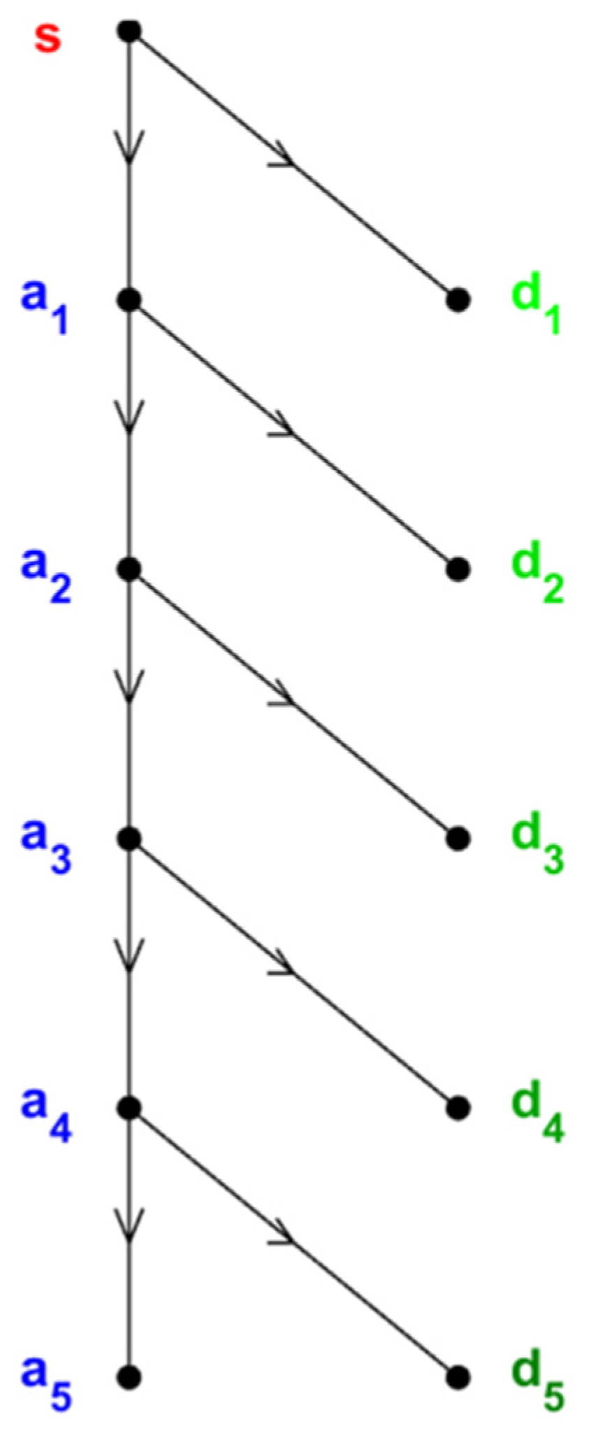
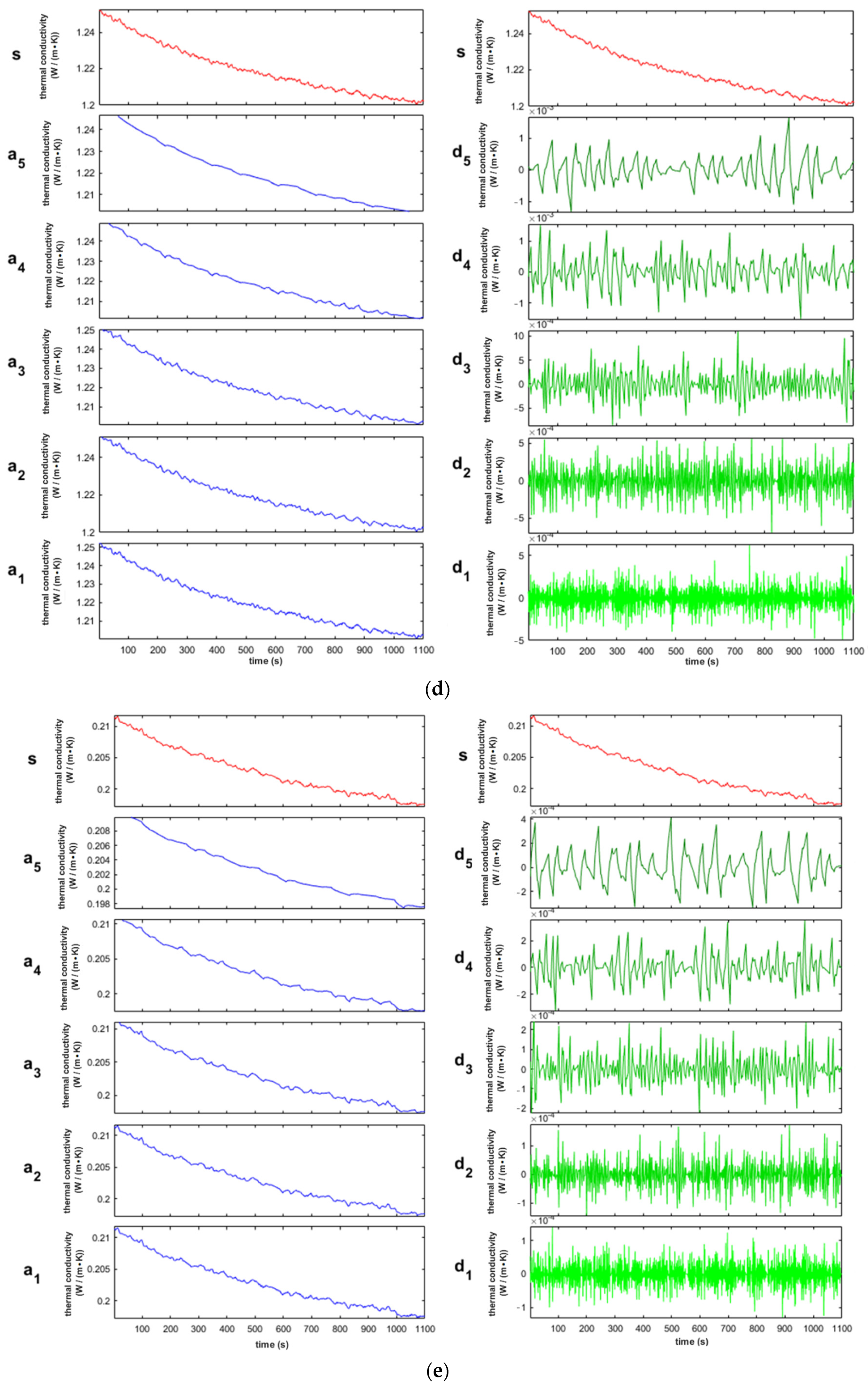
• First step: Selecting the right type of wavelet and decomposing the original S signal.
• Second step: Determining the thresholds at all levels of signal decomposition and threshold denoising of all detail components (high-frequency coefficients).
• Third step: Signal reconstruction.

The type of wavelet function should be selected in such a way that the wavelet is correlated with the signal [25]. Thus, it is possible to carry out the correct analysis and reconstruction of the signal. Multiresolution analysis allows the decomposition of the original signal S into approximation coefficients a_x and detail coefficients d_x. The approximation coefficients a_x represent the low-frequency components and the detail coefficients d_x represent the high-frequency ones [16,24]. Decomposition of the original signal S is a multilevel iterative process. Each subsequent iteration reduces the signal sampling frequency by a factor of two. Additionally, for each subsequent iteration, there is an expansion level index x greater by one, which corresponds to a two-fold reduction in resolution [24]. In the decomposition process of the original signal S, the subsequent approximations are then decomposed. It should be noted that with an increasing index x, the content of the information in the detail and approximation coefficients decreases.

In the process of denoising the original signal S, it is very important to set appropriate thresholds at all decomposition levels x in the range from 1 to x and to perform thresholding. There are two methods of thresholding: Soft and hard. Hard thresholding is a method that resets the coefficients to zero when their absolute values are less than a set threshold and the values of the other coefficients are not changed. In the case of soft thresholding, those coefficients with an absolute value lower than the specified threshold are reset to zero, but at the same time, the absolute values of the other coefficients are reduced by the threshold value. Therefore, the application of hard threshold elimination may cause discontinuity, while in the case of soft elimination, there is no discontinuity [24,25].

Signal reconstruction is carried out using the original approximations of the level x and appropriately defined detail coefficients at the levels from 0 to x [24,25].

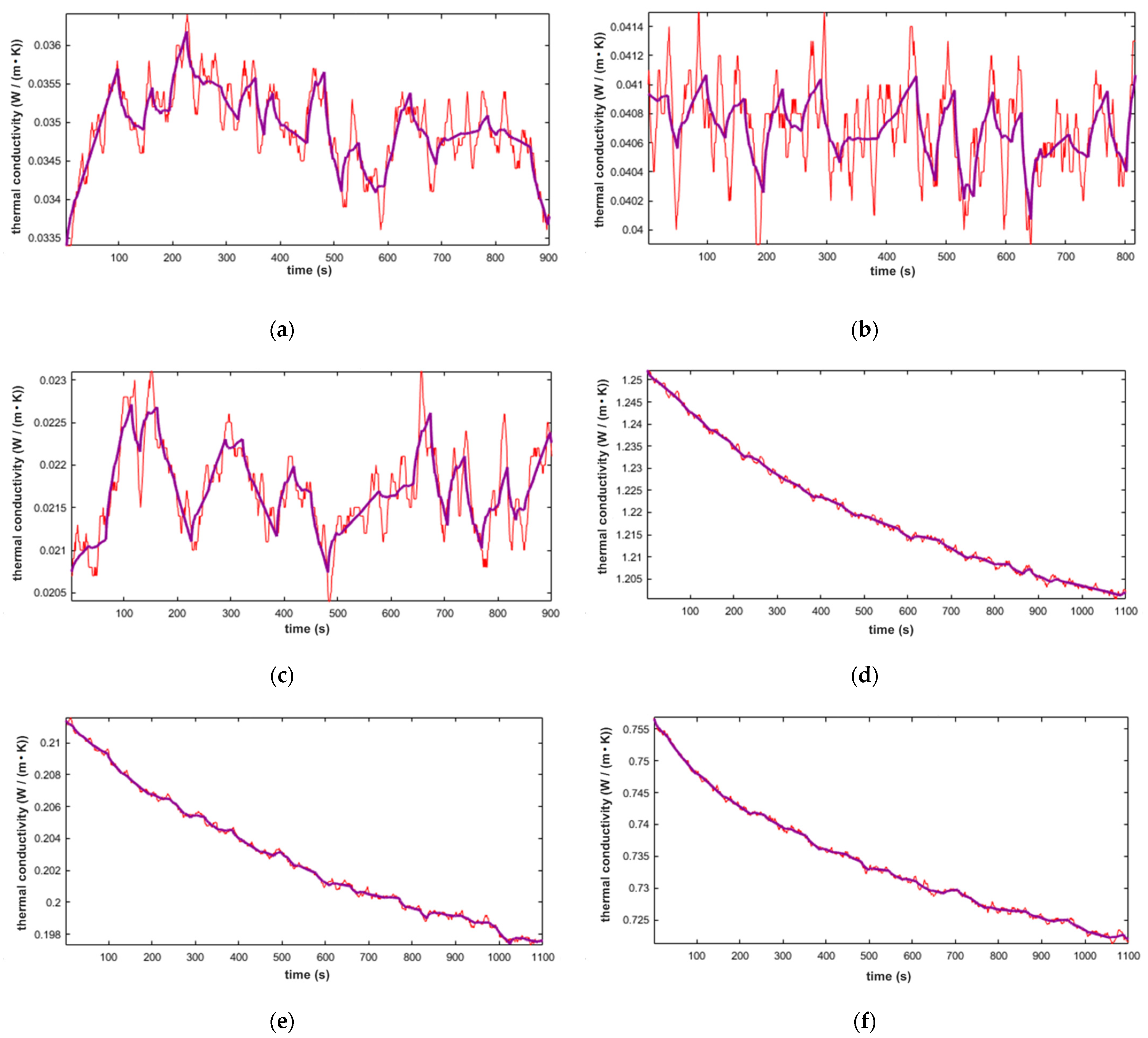
3. Results and Discussion

The time dependencies of the measured values of the temperature and heat flux, obtained in one of the experiments according to the standard procedure for the sample of organic glass SOL are presented in Figure 2 and Figure 3.

The zero point of the abscissa axis (Figure 2 and Figure 3) corresponds to the start of the thermal regime after the installation of the device on the test sample. After installing the device on the sample, the control system quickly creates a given temperature difference (Figure 2 and Figure 3). To achieve this aim, in the initial period of time, the power supplied to the sample was increased. As can be seen from the graph in Figure 2, the temperature difference stabilized 2 min after installation of the device on the sample and was then maintained at a stable level. The measured value of the heat flux continued to change, as can be seen in the graph of Figure 3, and after 20 min, the heat flux also stabilized, which served as an indicator to start the measurement.

Thus, 25 min (1500 s) after the start of the experiment, the thermal processes in the samples could be considered as stationary, and the device was considered to have entered the measurement mode [12].

Table 2. Measurement results obtained by the heat flow meter apparatus and the device for the express control of thermal conductivity.

Sample Number	Sample	Thermal Conductivity Measured by the Heat Flow Meter Apparatus (W/(m·K))	Thermal Conductivity Measured by the Express Control Device (W/(m·K))	Standard Deviation	Relative Error (%)
1	Organic glass SOL	0.1960	0.2022	0.0062	3.16
2	Optical glass TF-1	0.7230	0.7322	0.0092	1.27
3	Optical glass LK-5	1.1650	1.2172	0.0522	4.48
4	Polyurethane	0.0227	0.0217	0.0010	4.41
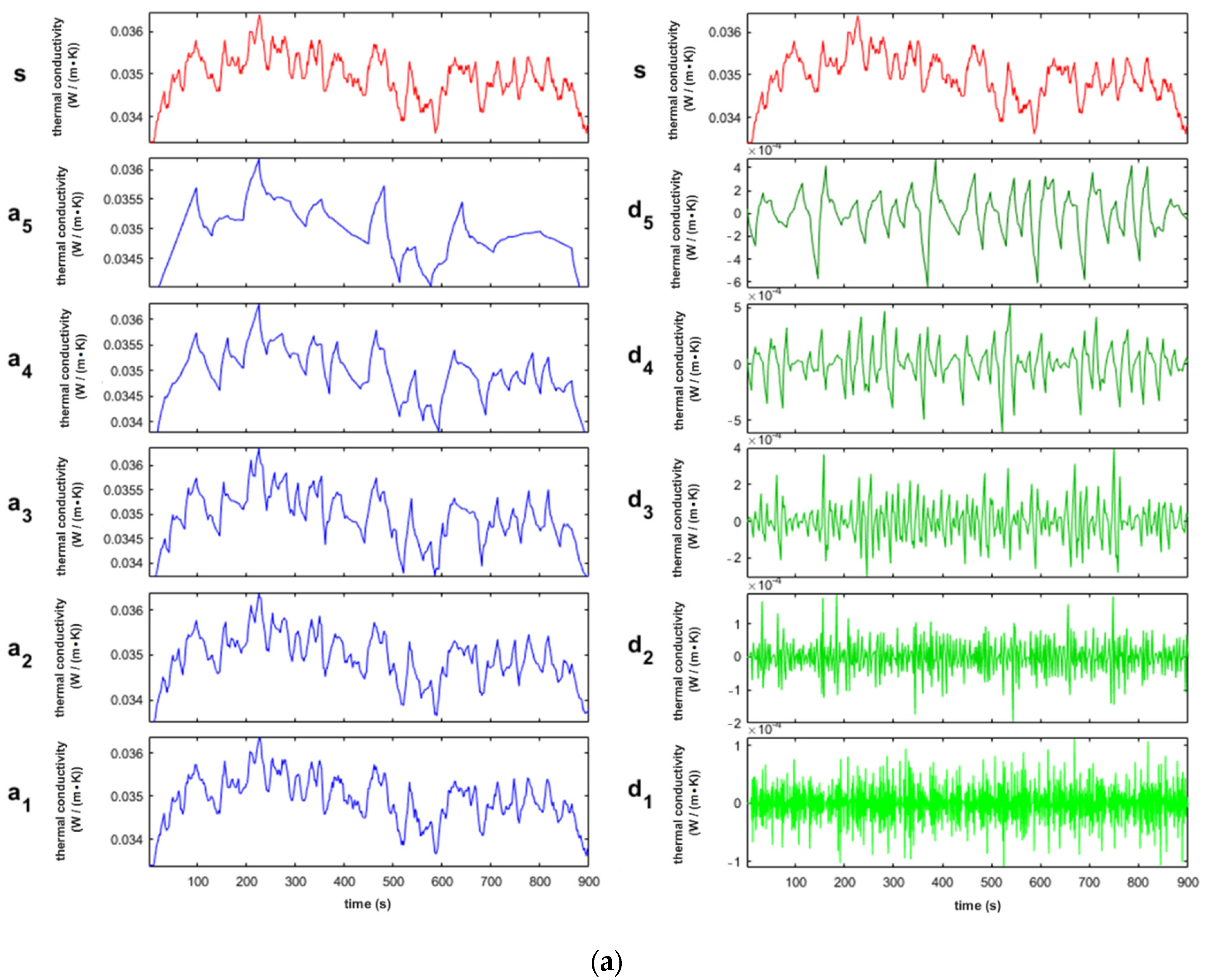
5	Extruded polystyrene (XPS)	0.0340	0.0349	0.0009	2.65
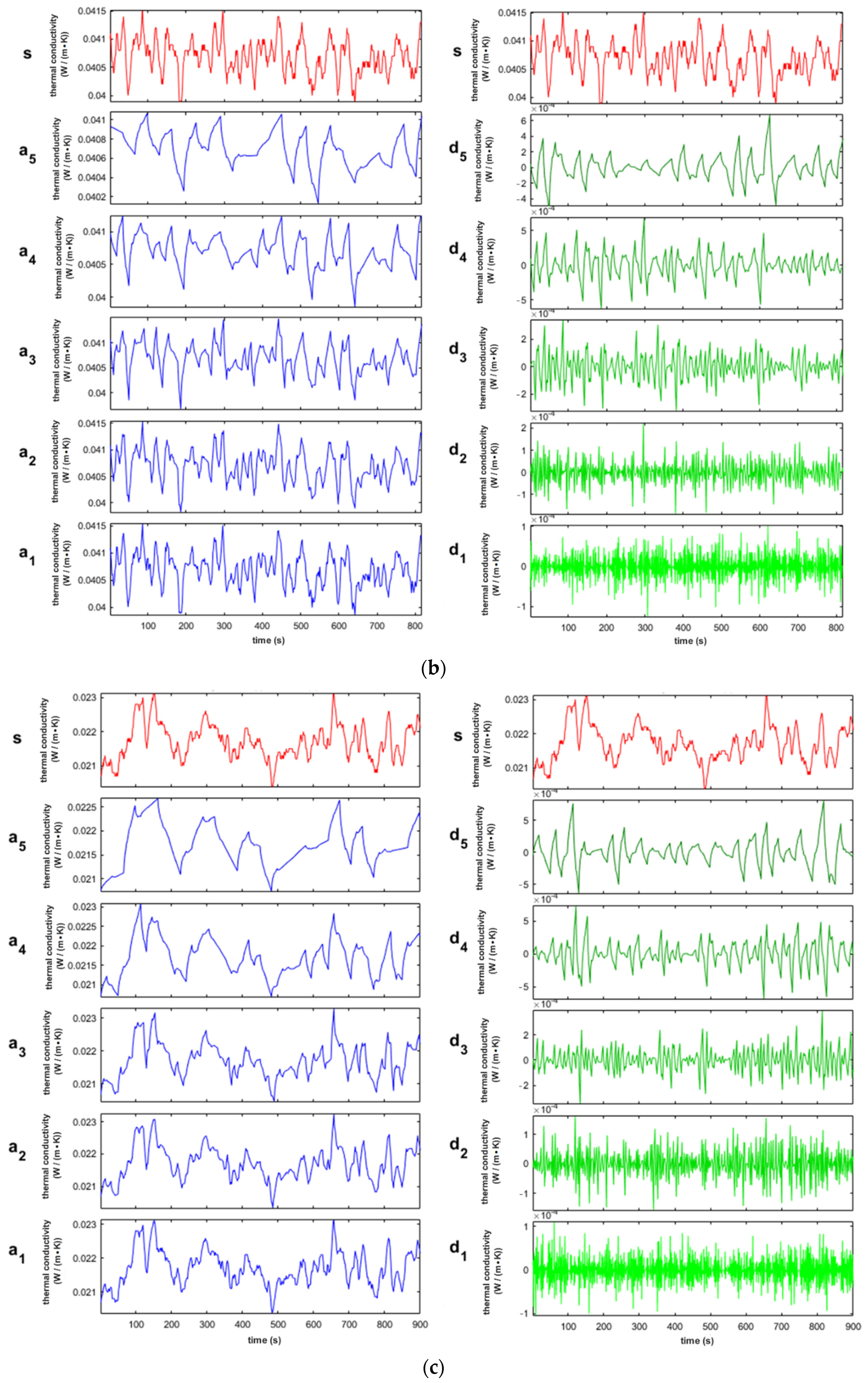
6	Expanded polystyrene (EPS)	0.0405	0.0407	0.0002	0.49
Remark. The values of the thermal conductivity correspond to the temperature of the sample (293 K).

presents the measurement results of the device for express control of the thermal conductivity, processed according to the standard procedure and by the heat flow meter apparatus [21], made according to ISO 8301 [2].

To improve the processing measurement information, wavelet transform was used, which allowed one to select a useful signal in the unstable mode. Therefore, data processing began in the 10th minute from the beginning of the experiment.

Thermal conductivity tests were conducted for the materials presented in Table 2. Six different original signals S were investigated. The analysis of the measurement results of the thermal conductivity of the glass for all variants was carried out using multiresolution analysis. The process of denoising the original signal S was used to remove noise and to obtain detailed information. The Daubechies wavelet of the order of 2 at decomposition level 5 was selected for investigation. This wavelet was characterized by a high signal correlation and a detailed reconstruction process of the original signal S. The value of the decomposition level was chosen in such a way that the details of the signal above decomposition level 5 could be ignored. Decomposition of the signal S resulted in its decomposition into individual details dx and approximations a_x. Figure 4 shows the wavelet decomposition process of the thermal conductivity signal, which was used in all six cases.

The measurement data were subjected to signal decomposition using the Daubechies wavelet of the order of 2 and are presented in Figure 5.

Each of the signals was decomposed into 10 components, including five detailed sub-signals and five approximate sub-signals. The detailed sub-signals d₁–d₅ represents the high-frequency components, while the approximate sub-signals a₁–a₅ represent the low-frequency components of the original signal S. The level of signal decomposition was determined in such a way that a number was selected above which details could be omitted. The original signals S are shown at the top of Figure 5a–f. Approximate sub-signals in all graphs are located in the right column and detailed sub-signals in the left column. In all of the characteristics (a–f), the approximate components a₅ are the changes in the low-frequency range of the original signal S. The detailed components d₄ and d₅ of all signals have sharper peaks than the detailed components d₁–d₃. The detailed components d₁ and d₂ in all original signals are dominant. The detailed components d₃–d₅ in signals (a) and (f) and the detailed components d₄ and d₅ in signals b–e are characterized by higher amplitudes.

The next step was thresholding at all levels of detail decomposition of the original signal S and performing soft threshold elimination. Signal reconstruction was performed using the signal approximation a₅ and detailed coefficients after the threshold elimination. The effect of denoising the thermal conductivity signal using the Daubechies wavelet of the order of 2 at decomposition level 5 is shown in Figure 6 (the original signal is marked in red, and the denoised signal is marked in violet).

In the measurement range of thermal conductivity less than 0.2 W/(m∙K), a comparison of the original (red line) and denoised (violet line) graphs shows a reduction of peaks and dips (Figure 6a–c). In addition, the average level of the signal stabilized at the 10 min point. This means that the measurements could be started from 10 min with the same error as testing for 25 min. In the measurement range of thermal conductivity from 0.2 to 1.4 W/(m∙K), a comparison of the original and denoised signals shows that we were unable to reduce the measurement time, but the peaks and dips were reduced (Figure 6d–f).

The results of the thermal conductivity measurement processed using wavelet transform are presented in

Table 3. Comparison of the measurement results for all materials processed according to the standard procedure with those processed using wavelet transform.

Sample Number	Sample	Thermal Conductivity (W/(m∙K))	Determined Thermal Conductivity Coefficient Using a db Wavelet of the Order of 2 at Decomposition Level 5 (W/(m∙K))	Time (s)	Standard Deviation	Relative Error (%)
1	Organic glass SOL	0.1960	0.2064	300	0.0072	5.3060
			0.2031	600	0.0056	3.6200
			0.1976	900	0.0038	0.8200
2	Optical glass TF-1	0.7230	0.7417	300	0.0140	2.5900
			0.7358	600	0.0134	1.7700
			0.7226	900	0.0089	0.0600
3	Optical glass LK-5	1.1650	1.2330	300	0.0317	5.8360
			1.2190	600	0.0196	4.6300
			1.2040	900	0.0140	3.3500
4	Polyurethane	0.0227	0.0218	300	0.0006	4.0132
			0.0217	600	0.0005	4.5286
			0.0217	900	0.0004	4.2907
5	Extruded polystyrene (XPS)	0.0340	0.0351	300	0.0006	3.3400
			0.0350	600	0.0005	2.9500
			0.0348	900	0.0005	2.3500
6	Expanded polystyrene (EPS)	0.0405	0.0409	300	0.0003	0.7010
			0.0406	600	0.0002	0.2500
			0.0406	900	0.0002	0.2500

.

The numerical values 300, 600, and 900 in the “Time” column correspond to the duration of recording the measurement information. From the data presented in Table 3, it follows that the application of the Daubechies wavelet of the order of 2 at decomposition level 5 for processing data decreases the thermal conductivity measurement’s relative error for the following samples: More than three times for organic glass SOL, more than 10 times for optical glass TF-1, and 1.3 times for optical glass LK-5. The relative error values of the measurement results processed using wavelet transform at a measurement information recording duration of 900 s (see Table 3) were compared to those processed according to the standard procedure (see Table 2). In the measurement range of the thermal conductivity from 0.2 to 1.4 W/(m∙K), if the measurement data recording started at the 10th minute and was carried out within 900 s (15 min), the application of wavelet transform allowed to reduce the measurement error due to the processing of a larger data array as compared to the standard procedure of data processing.

When the Daubechies wavelet of the order of 2 at decomposition level 5 was applied to the polyurethane, XPS, and EPS thermal conductivity measurement data, as shown in Table 3, it was sufficient to record for 300 s (5 min) while maintaining the same level of the measurement error. Thus, when studying thermal insulation materials, a duration of 15 min is sufficient for an experiment.

The obtained results indicate that due to the use of wavelet transform for the data of thermal conductivity measurement results, it is possible to achieve measurement accuracy at the level of laboratory tests while maintaining the duration of express control. In the case of thermal insulation materials, the duration of the experiment can be reduced twice while keeping the measurement accuracy.

4. Conclusions

The present article provided improved approaches to processing the thermal conductivity measurement data of insulation materials obtained by the abovementioned device for the express control of thermal conductivity based on the method of local heat influence. To achieve this aim, wavelet analysis was applied, and studies were carried out on three samples of the most common thermal insulation materials, i.e., polyurethane, extruded polystyrene, and expanded polystyrene. Additionally, optical and organic glass was investigated, as materials with a stable value of thermal conductivity.

As a result of these studies, it was found that for organic glass SOL and optical glass TF-1 and LK-5, for a thermal conductivity range greater than 0.2 W/(m∙K), the application of the Daubechies wavelet of the order of 2 at decomposition level 5 allows a reduction in fluctuations of the measured signals (reduction of the standard deviation). In the studies of thermal insulation materials with a thermal conductivity less than 0.2 W/(m∙K), a reduction of the standard deviation of the measurement results was obtained even when the data recording were carried out within 300 s; thus, the duration of the experiment can be reduced in twice.

The results of this study can be used to increase the accuracy in the express control of the thermal conductivity of insulation materials by improving the data processing. This approach does not require a change in the design of the measuring equipment or the use of additional tools and can be implemented in software. In the future, it is advisable to apply wavelet analysis to the signals of temperatures and heat fluxes separately during measurement, to recalibrate the device, and to make a special measurement mode for insulation materials.

References

- ISO 8302. Thermal Insulation—Determination of Steady-State Thermal Resistance and Related Properties—Guarded Hot Plate Apparatus; ISO: Geneva, Switzerland, 1991. [Google Scholar]
- ISO 8301. Thermal Insulation—Determination of Steady-State Thermal Resistance and Related Properties—Heat Flow Meter Apparatus; ISO: Geneva, Switzerland, 1991. [Google Scholar]
- Zhao, D.; Qiao, X.; Gu, X.; Jajja Ayub, S.; Yang, R. Measurement techniques for thermal conductivity and interfacial thermal conductance of bulk and thin film materials. J. Electron. Packag. 2016, 138, 040802. [Google Scholar] [CrossRef] [Green Version]
- Mathis, N. Transient thermal conductivity measurements: Comparison of destructive and nondestructive techniques. High Temp. High Press. 2000, 32, 321–327. Available online: https://www.ctherm.com/files/Transient_Thermal_Conductivity_Measurements.pdf (accessed on 28 May 2021).
- Ghadimi, A.; Saidur, R.; Metselaar, H.S.C. A review of nanofluid stability properties and characterization in stationary conditions. Int. J. Heat Mass Transf. 2011, 54, 4051–4068. [Google Scholar] [CrossRef]
- American Society of Heating, Refrigerating and Air-Conditioning Engineers. ASHRAE Handbook: Fundamentals; ASHRAE: Atlanta, GA, USA, 2001. [Google Scholar]
- Brzezinski, A.; Tleoubaev, A. Effects of Interface Resistance on Measurements of Thermal Conductivity of Composites and Polymers. In Proceedings of the 30th Annual Conference on Thermal Analysis and Applications (NATAS); Kociba, K.J., Ed.; B&K Publishing: Pittsburgh, PA, USA, 2002; pp. 512–517. [Google Scholar]
- Ruuska, T.; Vinha, J.; Kivioja, H. Measuring thermal conductivity and specific heat capacity values of inhomogeneous materials with a heat flow meter apparatus. J. Build. Eng. 2017, 9, 135–141. [Google Scholar] [CrossRef]
- Li, Y.; Shi, C.; Liu, J.; Liu, E.; Shao, J.; Chen, Z.; Dorantes-Gonzalez, D.J.; Hu, X. Improving the accuracy of the transient plane source method by correcting probe heat capacity and resistance influences. Meas. Sci. Technol. 2014, 25, 015006. [Google Scholar] [CrossRef]
- Pásztory, Z.; Anh Le, D.H. An overview of factors influencing thermal conductivity of building insulation materials. J. Build. Eng. 2021, 102604, 1–16. [Google Scholar] [CrossRef]
- Lakatos, Á.; Kalmár, F. Investigation of thickness and density dependence of thermal conductivity of expanded polystyrene insulation materials. Mater. Struct. 2013, 46, 1101–1105. [Google Scholar] [CrossRef] [Green Version]
- Hotra, O.; Dekusha, O. A device for thermal conductivity measurement based on the method of local heat influence. Przegląd Elektrotech. 2012, 88, 223–226. [Google Scholar]
- Gurav, M.; Sarik, S.; Singh, K.; Pendharkar, G.; Baghini, M.S. IITB_TDR: A portable TDR system with DWT based denoising for soil moisture measurement. Sens. Actuator A Phys. 2018, 283, 317–329. [Google Scholar] [CrossRef]
- An, M.; Liu, M.; Ma, Y.; Xu, X. Multi-scale vibration behavior of a graphite tube with an internal vapor–liquid–solid boiling flow. Powder Technol. 2016, 291, 201–213. [Google Scholar] [CrossRef]
- Oh, Y.Y.; Yun, S.T.; Yu, S.; Kim, H.J.; Jun, S.C. Characterization of Environmental Drivers Controlling the Baseline of Soil Surface CO2 Flux using Wavelet-based Multiresolution State-Space Model and Wavelet Denoising. Energy Procedia 2018, 154, 157–162. [Google Scholar] [CrossRef]
- Ch’ien, L.; Wang, Y.; Shi, A.; Li, F. Wavelet filtering algorithm for improved detection of a methane gas sensor based on non-dispersive infrared technology. Infrared. Phys. Technol. 2019, 99, 284–291. [Google Scholar] [CrossRef]
- Dong, H.; Nie, Y.; Cui, J.; Kou, W.; Zou, M.; Han, J.; Guan, X.; Yang, Z. A wavelet-based learning approach assisted multiscale analysis for estimating the effective thermal conductivities of particulate composites. Comput. Methods Appl. Mech. Eng. 2021, 374, 113591. [Google Scholar] [CrossRef]
- Anstett-Collina, F.; Goffart, J.; Mara, T.; Denis-Vidal, L. Sensitivity analysis of complex models: Coping with dynamic and static inputs. Reliab. Eng. Syst. Saf. 2015, 134, 268–275. [Google Scholar] [CrossRef] [Green Version]
- Gonga, M.; Wang, J.; Bai, Y.; Li, B.; Zhang, L. Heat load prediction of residential buildings based on discrete wavelet transform and tree-based ensemble learning. J. Build. Eng. 2020, 32, 101455. [Google Scholar] [CrossRef]
- Dekusha, O.; Burova, Z.; Kovtun, S.; Dekusha, H.; Ivanov, S. Information-Measuring Technologies in the Metrological Support of Thermal Conductivity Determination by Heat Flow Meter Apparatus. Stud. Syst. Decis. Control 2020, 298, 217–230. [Google Scholar] [CrossRef]
- Dekusha, L.; Kovtun, S.; Dekusha, O. Heat Flux Control in Non-stationary Conditions for Industry Applications. In Proceedings of the 2019 IEEE 2nd Ukraine Conference on Electrical and Computer Engineering (UKRCON), Lviv, Ukraine, 2–6 July 2019; pp. 601–605. [Google Scholar] [CrossRef]
- Babak, V.; Kovtun, S.; Dekusha, O. Information-measuring technologies in the metrological support of heat flux measurements. In Proceedings of the Third International Workshop on Computer Modeling and Intelligent Systems (CMIS-2020), Zaporizhzhia, Ukraine, 27 April–1 May 2020; Volume 2020, pp. 379–393. Available online: http://ceur-ws.org/Vol-2608/paper29.pdf (accessed on 28 May 2021).
- Ding, Y.; Nanba, T.; Miura, Y.; Osaka, A. Wavelet structural analysis of silica glasses manufactured by different methods. J. Non Cryst. Solids 1997, 222, 50–58. [Google Scholar] [CrossRef]
- Białasiewicz, J.T. Falki i Aproksymacje; WNT: Warsaw, Poland, 2000. [Google Scholar]
- Mallat, S.G. A theory for multiresolution signal decomposition: The wavelet representation. IEEE Trans. Pattern Anal. Mach. Intell. 1989, 11, 674–693. [Google Scholar] [CrossRef] [Green Version]