Article

Crowdsourcing Urban Air Temperature Data for Estimating Urban Heat Island and Building Heating/Cooling Load in London

1
Department of Meteorology, University of Reading, Reading RG6 6UR, UK
2
School of the Built Environment, University of Reading, Reading RG6 6UR, UK
3
College of Electronics and Information Engineering, Shenzhen University, Shenzhen 518061, China
*
Author to whom correspondence should be addressed.
Energies 2021, 14(16), 5208; https://doi.org/10.3390/en14165208
Submission received: 8 June 2021 / Revised: 5 August 2021 / Accepted: 13 August 2021 / Published: 23 August 2021
(This article belongs to the Special Issue Resilience and Climate Adaptability of Buildings and Urban Areas)

Abstract

:
Urban heat island (UHI) effects significantly impact building energy. Traditional UHI investigation methods are often incapable of providing the high spatial density of observations required to distinguish small-scale temperature differences in the UHI. Crowdsourcing offers a solution. Building cooling/heating load in 2018 has been estimated in London, UK, using crowdsourced data from over 1300 Netatmo personal weather stations. The local climate zone (LCZ) scheme was used to classify the different urban environments of London (UK). Inter-LCZ temperature differences are found to be generally consistent with LCZ temperature definitions. Analysis of cooling degree hours in July shows LCZ 2 (the densest urban LCZ in London) had the highest cooling demand, with a total of 1550 cooling degree hours. The suburban related LCZs 5 and 6 and rural LCZs B and D all had about 80% of the demand of LCZ 2. In December, the rural LCZs A, B and D had the greatest heating demand, with all recording around 5750 heating degree hours. Urban LCZs 2, 5 and 6 had 91%, 86% and 95% of the heating demand of LCZ D, respectively. This study has highlighted both advantages and issues with using crowdsourced data for urban climate and building energy research.

1. Introduction

Energy resources in a building usually refer to electricity, natural gas and district heating supply [1]. It accounts for about 40% of the global energy consumption and contribute over 30% of the CO2 emissions [2]. The building energy consumption over the world is increasing due to climate change, urbanization and other factors. The tonnes oil equivalent has tripled from 1970 to 2010. Meanwhile, fossil fuels (oil, gas and coal) account for 90% of global primary energy production [3], which is one of major contributors of carbon emissions. The steadily increasing amount of energy consumption and carbon emissions has raised great challenges for sustainable development such as greenhouse gas emissions, air pollution, and reliable energy supply.
It has been widely acknowledged that urban heat islands (UHIs) have a significant impact on building energy consumption. The warmer urban temperatures associated with UHIs could increase building energy required for cooling and decrease energy required for heating. For example, Santamouris et al. [4] noted that in Athens, where the mean UHI exceeds 10 °C, the UHI is capable of doubling the urban building cooling load and can triple the peak electricity load for cooling purposes. Conversely, during the winter, urban buildings’ heating load can be reduced by up to 30%. Kolokotroni et al. [5] showed that an office located in a rural area had only 84% of the cooling demand of one in an urban area. In the UK heating (cooling) demand increases (decreases) with distance from London city centre, although this trend is not uniform with direction [6]. Kolokotroni et al. [6] discovered that, in addition to distance from the city centre, energy demand is dependent on several site-specific parameters, especially parameters related to vegetation cover and building density surrounding that site. For example, the variation in annual heating demand of different built forms could be between 1.1 and 7.3%, the lowest heat demand is the courtyard in UK [7]. The impacts of the UHI on building energy can lead to both economic savings from the reduced need to warm buildings [8] but also can incur vast economic costs due to the additional requirement to cool buildings. In Hong Kong, the sensible cooling demand of the urban buildings was approximately twice that of the rural one, and the latent cooling demand could be up to 96% higher [9]. In the US, the summer cost of UHI alone is up to $1 billion, with 3–8% of energy demand in urban areas used to compensate for the heat island [10]. Furthermore, future climate change is expected to increase the cooling load of buildings [11,12], exemplifying the importance of understanding and planning for the influence of the UHI on building energy.
Understanding the small-scale heterogeneities will give a complete knowledge of the impact of the urban form on building energy. Traditional methods of UHI investigation include station pair, transect methods and urban climate modeling. Guattari et al. [13] found that an average increase of cooling energy demand of about 30% and an average reduction of heating energy demand of about 11% in Rome based on the meteorological data.
However, these methods offer limited spatial and/or temporal availability of data [14]. For example, modeled UHI impacts on building energy consumption are sensitive to the selection of stations and the uncertainty could be reduced by using the temperature from multiple stations, but most literature studies only used one or two stations as rural stations and the number of weather stations installed in the city is limited. Crowdsourcing can provide a high spatial density of data and a continuous, long time series, for free. Crowdsourcing is defined as obtaining data or information by enlisting the services of a (potentially large) number of people and/or from a range of public sensors, typically connected via the internet. It is a relatively new form of data collection for the atmospheric sciences but is one with great potential [15]. The high spatial density of measurements it can provide the potential to overcome previous limitations of urban climate investigation [16]. Meteorological data collection using crowdsourcing has manifested itself in several ways, including using phone battery temperature to derive air temperature [17,18] and mapping snow depth using social media [19]. However, of particular interest to this study is the use of Citizen Weather Stations (CWS). These are weather stations set up by members of the public for personal interest or education, not because it’s their profession [20]. Mass production of affordable and user-friendly stations has contributed greatly to a meteoric increase in the usage of CWS in recent years [21].
Another useful tool in urban climate research is the local climate zone (LCZ) scheme (as shown in Figure 1). Fenner et al. [22] used CWS data to show significant differences between LCZs, with consistent results in previous literature relating to LCZs and the urban heat island. CWS temperature measurements have also proved to be consistent with that of professionally run reference stations [22,23]. Nonetheless, using CWS for scientific research does provide a unique set of challenges that must be dealt with. Firstly, there is wildly varying data availability that can originate from issues with collection of data, or an interruption of the connection of the station to the internet [24]. Most importantly, the lack of meta-data from CWS’s makes it impossible to know the quality of the data a station. This means a quality check must be implemented on the data before it can be used. Despite these caveats, crowdsourcing is a highly promising tool for urban climate research and could be the only feasible mode of improving the spatial density of meteorological measurements in urban areas [14]. The potential of crowdsourcing is still being realized as crowdsourced weather data never has been used before to estimate LCZ variations in building energy.
This study will use crowdsourced data from ‘Netatmo’ personal weather stations to investigate temperature characteristics between LCZs in Greater London, UK, and the surrounding area. It is investigated whether these LCZ characteristics are consistent with the understanding and definitions of LCZs. The meteorological data is then applied to determine building energy usage in each LCZ. This will advance knowledge of the impact of urban form on these factors, which can be applied to city planning. Moreover, it also aims to highlight some of the issues related to using crowdsourced data. Although the UHI has been studied for almost two centuries, both crowdsourcing meteorological data and the local climate zone scheme are relatively new techniques. They are both highly promising concepts and so must be applied and tested as much as possible to improve the methods of their usage and unlock their potential.
The rest of this paper is organized as follows: Section 2 briefly introduces the study data, including crowdsourced data, weather data, Local climate zone (LCZ) data and heating/cooling load, and presents the details of quality check of the crowdsourced data. Section 3 presents the main results. The discussion part is presented in Section 4. We conclude and discuss the future work in Section 5.

2. Materials and Methods

2.1. Study Area and Time Period

The city studied was Greater London, UK, which has a population of 8.25 million [25], making it one of the largest cities in Europe. London is located in the mid-latitudes and has a Kppen-Geiger climate classification of Cfb: warm temperature, fully humid with warm summers [26]. Data was collected for the approximate region bound by the M25 orbital motorway. This was considered the area within in a box with coordinates of 51.245° latitude, −0.558° longitude at its southwest corner, and 51.721° latitude, 0.337° longitude at its northeast corner. Therefore, data collected includes both Greater London and its surroundings.
Data was collected from the 5 of July 2018 until 31 of December 2018. This is inclusive of several weeks of a heatwave in the UK that brought above-average temperatures for much of the summer. These anomalously high temperatures persisted up from 22 of June until the 8 of August [27]. Over this period temperatures exceeded 30 °C in some places in the UK on numerous days [27]. These kinds of heatwave events could significantly increase building cooling demand [28]. Temperatures for the remaining studied months remained close to the mean temperature from 1981 to 2010, although November and December were milder than average, with positive temperature anomalies of 1.1 °C and 1.9 °C, respectively [27].

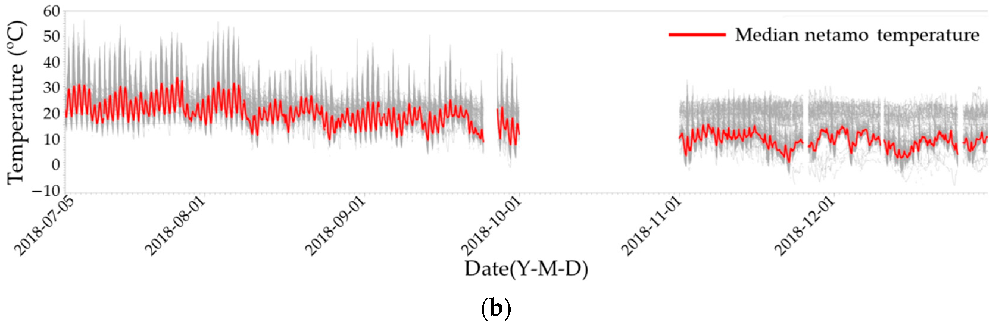
2.2. Crowdsourced Data, Data Acquisition and Quality Check

The crowdsourced data was obtained from ‘Netatmo smart home weather stations’ (Netatmo, Boulogne-Billancourt, France). These consist of two modules i.e., the indoor and outdoor ones. The outdoor module measures several variables including temperature, relative humidity, and pressure, with an anemometer and rain gauge also available as optional extras. The outdoor module transmits to the indoor module, which is connected to the internet whereby the users can view the data recorded by their station on a mobile app. Furthermore, the users can choose to publicly display the data on the ‘Netatmo weather map’ (https://weathermap.netatmo.com/, accessed on 2 January 2019). Netatmo stations are used extensively worldwide, especially in European cities. For example, data from a total of 1303 stations were obtained in this study. This high density of observations is important for the progression of the investigation of small-scale variations within UHI’s and therefore its impact on building energy. Furthermore, the accuracy of the temperature sensor of Netatmo stations has been tested and verified by Meier et al. [24]. Meier et al. [24] placed Netatmo stations in a climate chamber and compared temperature measurements to that of a reference sensor. This revealed that the Netatmo sensor was within the manufacturer’s accuracy specification of 0.3 °C. However, it should also be noted that a Netatmo station placed in a Stevenson screen next to a professionally managed station showed some considerable differences. Differences were greatest during the morning time when the Netatmo measured lower temperatures, likely due to its slower thermal response and differences in ventilation between the two apparatus [24]. Meier et al. [24] also noted that Netatmo had the additional advantage over several other crowdsourcing methods in that all stations are the same. Therefore, sensor errors should be consistent for all stations. Conversely, this is not true for other crowdsourcing methods such as Weather Underground [29], which use multiple station types.
Netatmo does not store any station data but data can be acquired in real-time through the Netatmo ‘Application Programming Interface’ (API). The Netatmo API provides numerous methods of data collection, and for this study, the ‘get public data’ method was used. This method returns instantaneous data from all stations within a specified area. As there is a limit on the number of stations that can be returned from a specified area, the study area was divided into 25 tiles, with a request made to the API for each tile on an hourly basis. The station ID, latitude, longitude, temperature, and relative humidity were obtained. Any stations that changed location throughout the study were considered a new station and assigned a new ID code. As previously mentioned in Section 2.1, the quality of each Netatmo measurement cannot be known, largely due to the lack of meta-data provided for each station. Misuse of stations can easily lead to errors in meteorological measurements. For example, radiation errors due to solar heating can arise from stations being placed in areas that are exposed to direct sunlight. Another potential misuse is that users can set up their outdoor modules indoors. Furthermore, failure of the Netatmo server, or the collecting server, can lead to chunks of missing data from all stations [24]. Hence, to ensure the analysed data has a good accuracy, a quality check (QC) must be implemented. For this study, the QC method devised by Napoly et al. [23] was used. This statistically-based method is divided into seven steps (briefly outlined in Table 1), which are designed to eliminate all the common issues associated with using CWS data.
In October, less than 80% of daily values are available, due to collection errors in this month. The option that to correct temperature readings by height was not carried out. This was because the correction presents an additional source of uncertainty as it corrects by the standard atmospheric lapse rate of 0.0065 K m−1, which is not valid at all times. In addition, the topography of the studied area is relatively uniform, so the inclusion of this correction would not have led to dramatic changes in temperature.
Table 1. Brief description of the levels of the quality check (QC) that was used for Netatmo data in this study. Table adapted from Napoly et al. [23].
QC LevelBrief Description of Procedure
M1Flag common locations to eliminate stations broadcasting IP address location
M2Flag upper and lower part of the hourly distribution
M3Flag month if M2 flagged > 20% of the month
M4Targets indoor stations by omitting stations that have a Pearson correlation coefficient between the station and the median of all CWS’s < 0.9
O1Linear interpolation of hourly values
O2Flag day if <80% of hourly values available
O3Flag month if <80% of daily values available

2.3. Reference Weather Data

Reference weather data was acquired from UK Met Office operated weather stations, via the Met Office Integrated Data Archive Systems (MIDAS) dataset [30] in order to conduct verification of the Netatmo data. Seven stations are located in the study area (indicated in Figure 2). UK hourly weather observation data [31] was downloaded for these stations. The name, location, and LCZ classification (as shown in Figure 1) of these sites can be found in Table 2. All the stations take measurements automatically from instrumentation contained within a Stevenson screen, elevated 1.25 m off the ground [32]. The inter-LCZ temperature trends observed by crowdsourced data will be validated by the reference data obtained from professionally run stations.
Table 2. Station name, coordinates and local climate zone (LCZ) classification of each Met Office operated reference station used in this study. Data from these stations were compared to crowdsourced data in order to test the validity of crowdsourced data.
Station NameLatitudeLongitudeLCZ Scheme 1
Hampton W Wks51.4114−0.376525
Heathrow51.4787−0.44904D
Kenley Airfield51.3035−0.08994D
Kew Gardens51.4813−0.29276B
London: St James’s Park51.5042−0.129486
Northolt51.5481−0.41534D
London City51.52080.07579D
1 As shown in Figure 1.
Figure 1. Definitions of the LCZs (image from Bechtel et al. [33], adapted from Stewart and Oke [34].
Energies 14 05208 g001

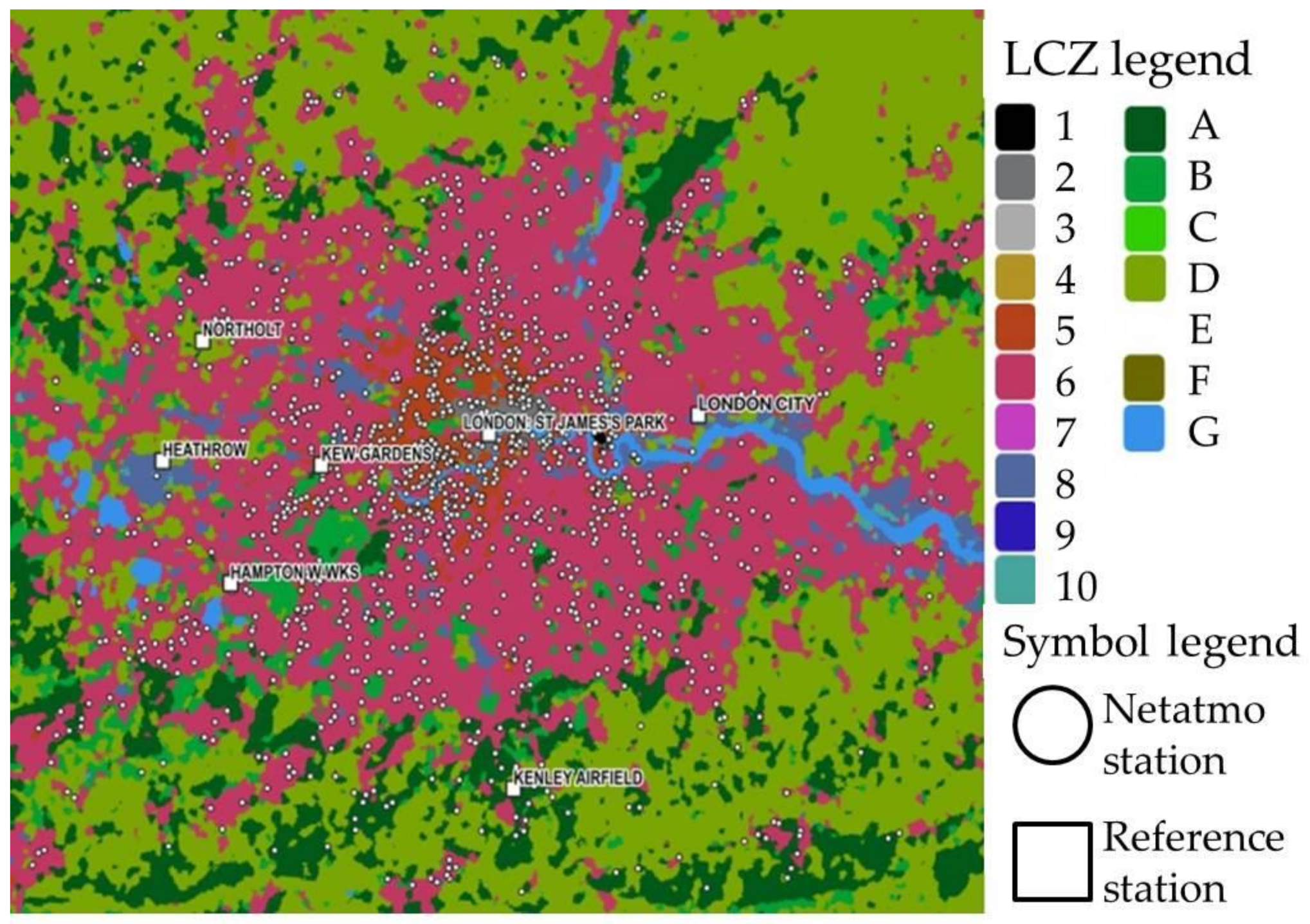
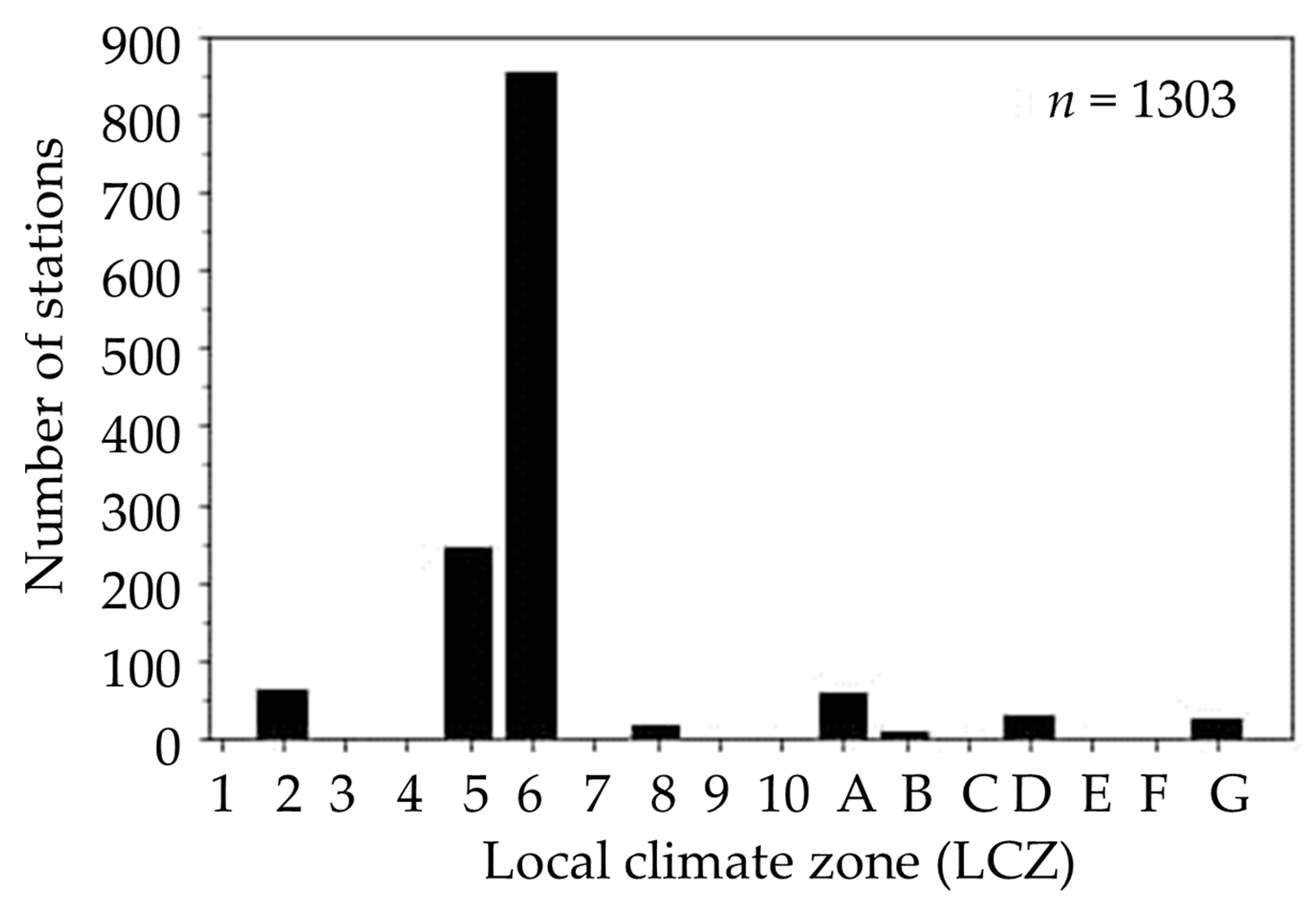
2.4. Local Climate Zone (LCZ) Data

The local climate zone (LCZ) scheme categorises landscapes into zones of uniform surface cover, structure, material, and human activity [34]. The goal of the LCZ scheme is to improve the accuracy and consistency of urban climate reporting and aid in integrating urban climate knowledge with city planning. There are 17 LCZs (seen in Figure 1), with different zones having different thermal characteristics. Zones with very different characteristics can have temperature differences exceeding 5 °C [34].
Local climate zone data was obtained from the World Urban Database and Access Portal Tools (WUDAPT) [35]. Local city experts, with the aid of satellite imagery, generate such LCZ maps using a method that was first hypothesized by Bechtel and Daneke [36] and refined by Bechtel et al. [37]. The London LCZ map was downloaded from the WUDAPT website (http://www.wudapt.org/, accessed on 29 January 2019). The map is in the form of a GeoTiff file, containing a raster map, with 100 m x 100 m pixels, of LCZs.
Figure 2 shows the LCZ map of London with the locations of every station collected throughout the study. Using tools in QGIS, each station was assigned an LCZ value based on the raster value of the pixel that it is within. The majority of Netatmo stations are classified as being in LCZs 5 (open mid-rise) and 6 (open low-rise) (as shown in Figure 3), which are associated with suburban areas. This is to be expected as most Netatmo owners will have disposable income and enough yard space for a CWS, both of which are typical for suburban areas. There are also stations present in the urban LCZs 2 (compact mid-rise), 8 (large low-rise), and 10 (heavy industry) and the rural LCZs A (dense trees), B (scattered trees), and D (low plants). There are some stations present in LCZ G (water), which may be installed in boats. As these are not our main interests, results from this LCZ are not mentioned further. Discussion of the possible reasons for and implications of this are considered further in Section 4. After this, stations that had heterogeneous land cover surrounding them were eliminated from the study, as ensuring temperature measurements were not influenced by different surrounding LCZs. This was achieved by using a similar approach to that used by Fenner et al. [22]. Any stations that 80% or more of the pixels within a 250 m radius were a different LCZ to the LCZ that the station was in were disregarded. This was also carried out for reference stations, but with a cut-off of 50% as opposed to 80%. The reason for this lower cut-off is that almost all the reference stations had high LCZ variability surrounding them, so the cut-off was reduced so that there were still several usable reference stations. An additional advantage of carrying this out is that it reduces the chance of a station being classified into the wrong LCZ. In theory, a station can be located within a pixel that contains two different land surfaces. In this case, the classification of the pixel may not cohere to the stations’ underlying surface. Also, if the location of the station is marginally incorrect, or the precision of the co-ordinates is too low, it could be classified into the wrong LCZ. Eliminating stations with highly variable surroundings should mitigate this. This process reduced the number of available Netamo stations by 320, from the original 1303. Therefore, approximately a quarter of stations were eliminated even before the QC was carried out. Furthermore, London Heathrow, Kenley Airfield, and London St James’s Park reference stations were eliminated.
Figure 2. The LCZ map of London with positions of all Netatmo stations (white circles) from which data was collected throughout this study. Labeled reference stations are also indicated by white squares.
Energies 14 05208 g002
Figure 3. The number of Netatmo stations in each LCZ, throughout the study. n represents the total number of stations from which data was collected.
Energies 14 05208 g003

2.5. Indicators for Determining Inter-LCZ Temperature Difference and Building Heating/Cooling Load

Data with the highest quality (Flag month if >80% of daily values available) after quality check [23] was analysed. For each station, the mean station temperature (Tmean), mean daily minimum temperature (Tmin), and mean daily maximum temperature (Tmax) was calculated for each month. The mean daily diurnal temperature range (DTR) was also evaluated by calculating the maximum temperature minus the minimum temperature for each day and finding the average over the month. The mean value of every station in each LCZ was then obtained. The same process was executed for the reference stations. Box plots for these variables were also computed for each LCZ in which ten or more stations were present. This allows for investigation into the thermal properties of different urban surfaces.
Stewart and Oke [34] suggest that, under the LCZ scheme, UHI magnitude could be defined as an LCZ temperature difference. Ideally, this would be defined as the temperature difference between LCZ 1 (compact high-rise) and LCZ D (low plants); however, according to the LCZ map from WUDAPT, LCZ 1 is not present in London. Therefore, for this study UHI magnitude has been defined as the temperature difference between LCZ 2 (compact midrise) and LCZ D.
To evaluate the UHI impact on building energy, the concept of heating and cooling degree hours (HDH/CDH), which is analogous to heating and cooling degree days, has been used. Degree hours are a simple and repeatable indicator of estimating and monitoring the energy consumption of buildings due to space heating and cooling. Degree hours can provide an approximation for building energy usage, although actual energy usage will vary depending on building-specific properties, such as casual gains, thermal capacity, and room moisture content [38]. The application of degree hours depends on the ‘base temperature’ (Tb). This is a balance point temperature at which outdoor ambient is sufficiently high (low) enough such that there is no need for additional heating (cooling). Tb varies between regions with different climates, but for the UK 15.5 °C is commonly used as Tb for HDH and 22 °C for CDH [39]. Degree hours are essentially an hourly summation of how many degrees the outdoor air temperature is above or below Tb. However, an issue that is particularly problematic for crowdsourced data, is that the number of hours recorded varies between stations, due to intermittent failures in the transmitting of data to the Netatmo API. Therefore, the degree hours have been normalised by the number of hours the station recorded. Following this, it has been multiplied by the maximum number of available hours for the studied period. Consequently, the CDH and HDH are defined mathematically in Equations (1) and (2), respectively:
CDH = j = t start j =   t end T j Tb   ( ( T j Tb ) > 0 ) n meas × n max
HDH = j = t start j =   t end Tb T j   ( ( Tb T j ) > 0 ) n meas × n max
where   t start is the starting time for degree hours to be calculated,   t end is the end time, T j is the temperature at time j and Tb is the base temperature, n meas is the number of measurements made by the station between   t start and t end , and n max is the maximum possible hourly measurements within this time frame.

3. Results

3.1. Effect of the Quality Control

The quality check method was validated on the cities of Berlin (Germany) and Toulouse (France) by Napoly et al. [23], and the proportion of the eliminated data at each level were recorded. The similar process was done for London data, and the results are shown in Table 3. From level M1 to O2, a similar proportion of data was eliminated in this study to the other two cities. Levels M1 to M4 consist of a statistical test to eliminate erroneous measurement. The similar result indicates the intrinsic quality of data collected from London is comparable to that of Berlin and Toulouse. The remaining steps (O1–O3) are focused on the availability of the data of each station. Level O3 eliminated a considerable amount more data in this study compared to the cities studied by Napoly et al. [23]. At level O2, about 75% of data remained for all three cities, whereas at O3 London had just 49.56% remaining, when Berlin and Toulouse had 58.54% and 57.41% remaining, respectively. Level O3 omits stations that have less than 80% of data in the month. The large difference between O2 and O3 indicates that the data collection was more intermittent or inconsistent in London than that of Napoly et al. [23]. This is likely due to intermittent errors in the script collecting data, or problems related to the tile size submitted to the API being too large. Figure 4 draws the hourly temperatures over the study period for all Netatmo stations and stations that passed the O3 level of the quality check and shows a clear improvement in the quality of data. The time series of the raw Netatmo data (Figure 4a) shows some unrealistic temperature readings exceeding 55 °C, likely obtained from stations that have been left in direct sunlight. Very little diurnal variation of the daily temperature can also be found, which may be contributed to the station being left indoors. Figure 4b shows the time series of Netatmo stations that passed level O3 of the QC. At this level, neither of these characteristic errors is visible, with much more realistic temperature readings and a spread much closer to the median temperature.
Table 3. The amount of crowdsourced temperature data remaining after each step of the quality check for London and two cities (Berlin and Toulouse) tested by Napoly et al. [23].
QC LevelRemaining Data in Each City (%)
LondonBerlin
(Napoly et al. 2018)
Toulouse
(Napoly et al. 2018)
M197.7199.8498.26
M287.0789.3888.91
M385.9782.4181.65
M485.0282.2181.45
O189.7283.7486.47
O274.8475.0476.71
O349.5658.5457.41
Figure 4. Hourly temperatures over the study period for all Netatmo stations (a) and stations that passed the O3 level of the quality check (b). Grey lines are a time series for each station and the red line represents the median of the stations.
Energies 14 05208 g004aEnergies 14 05208 g004b

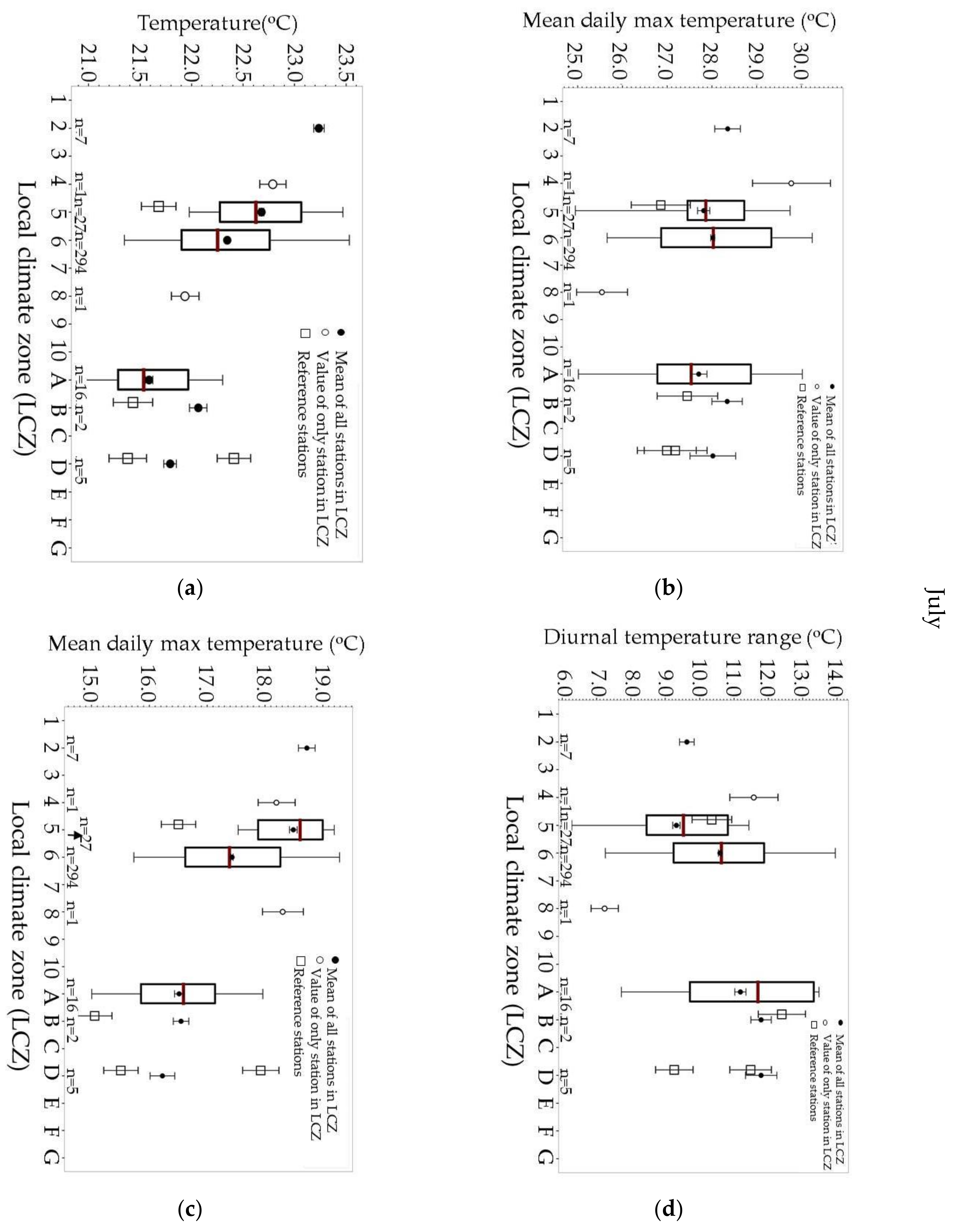
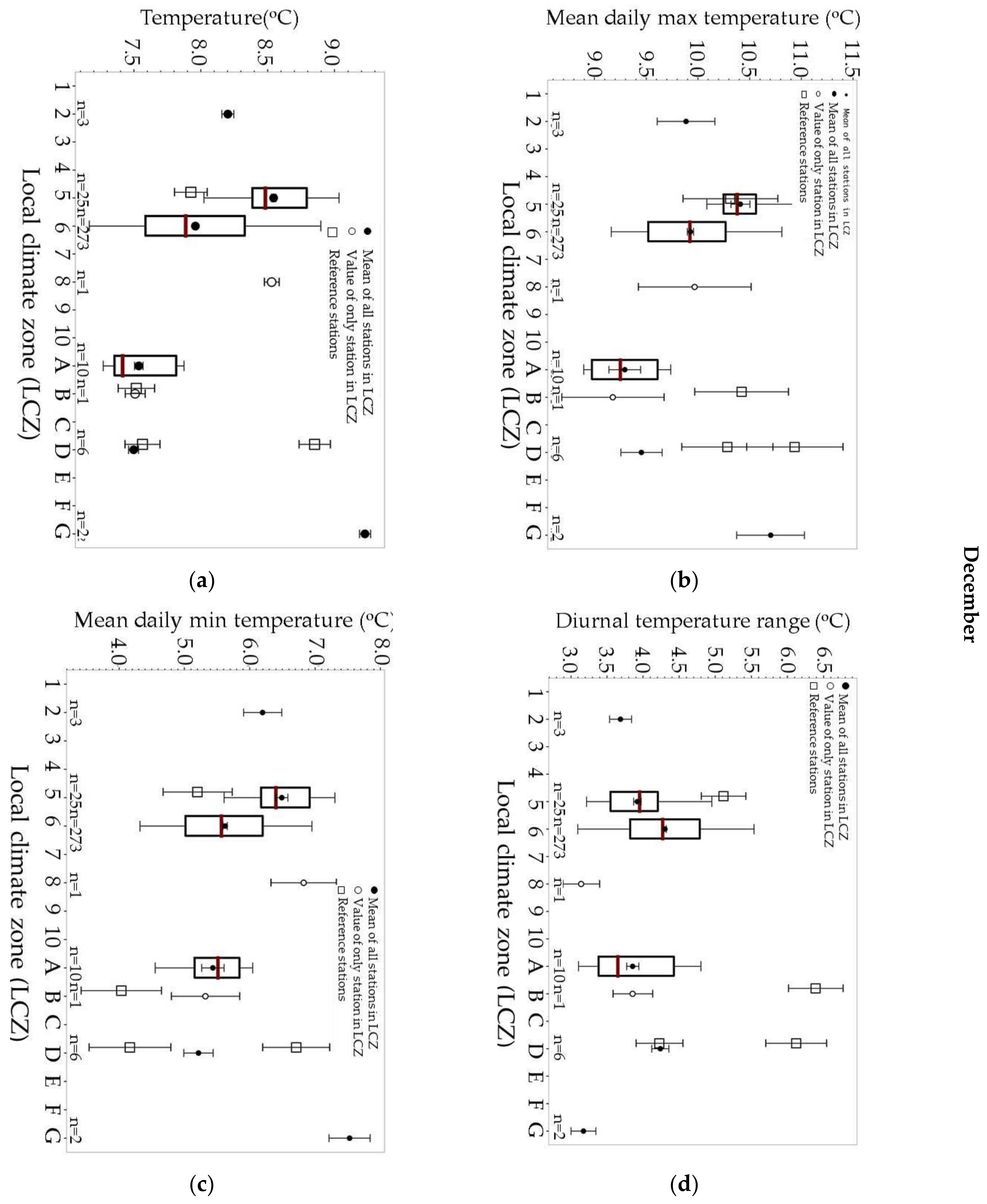
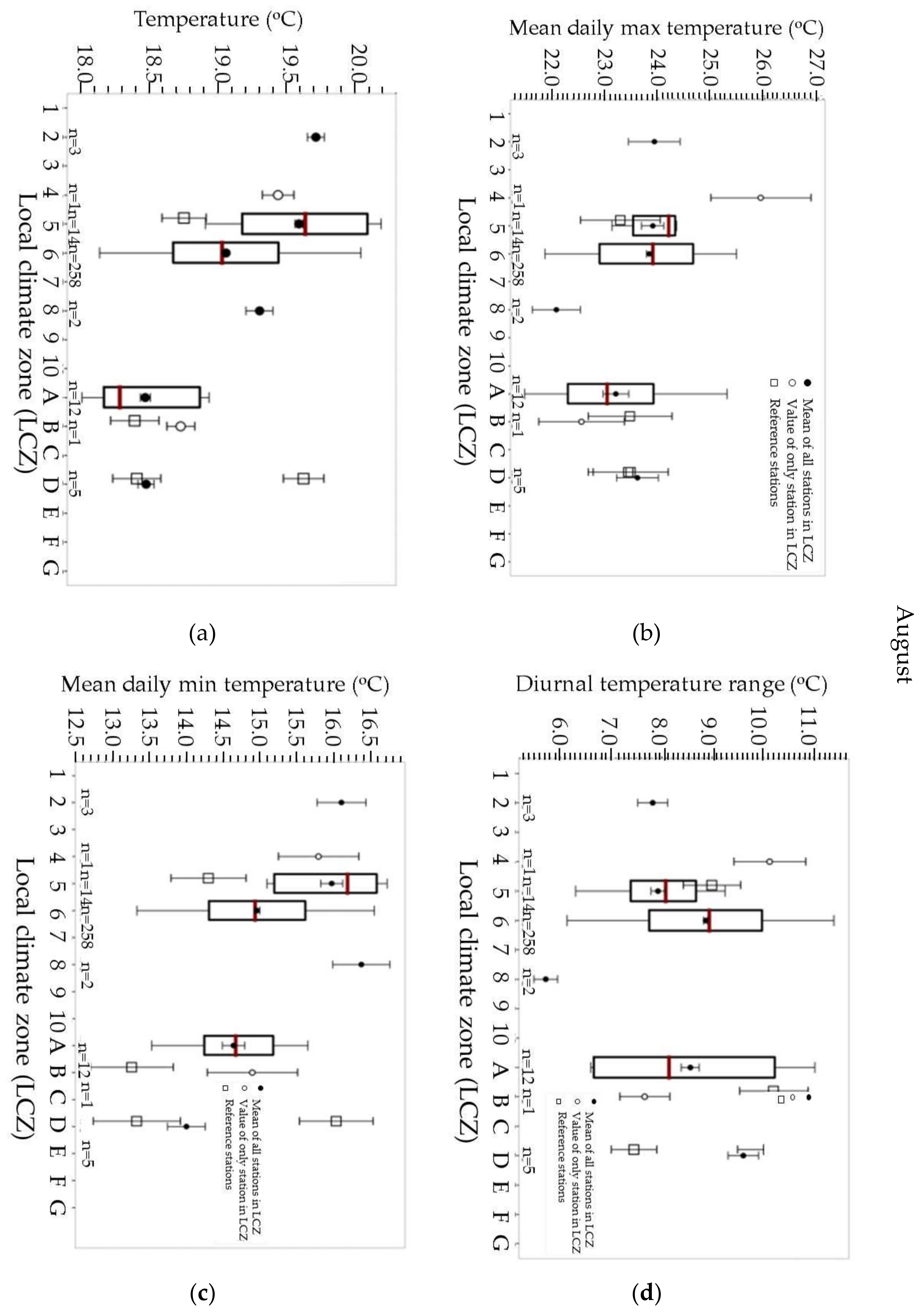
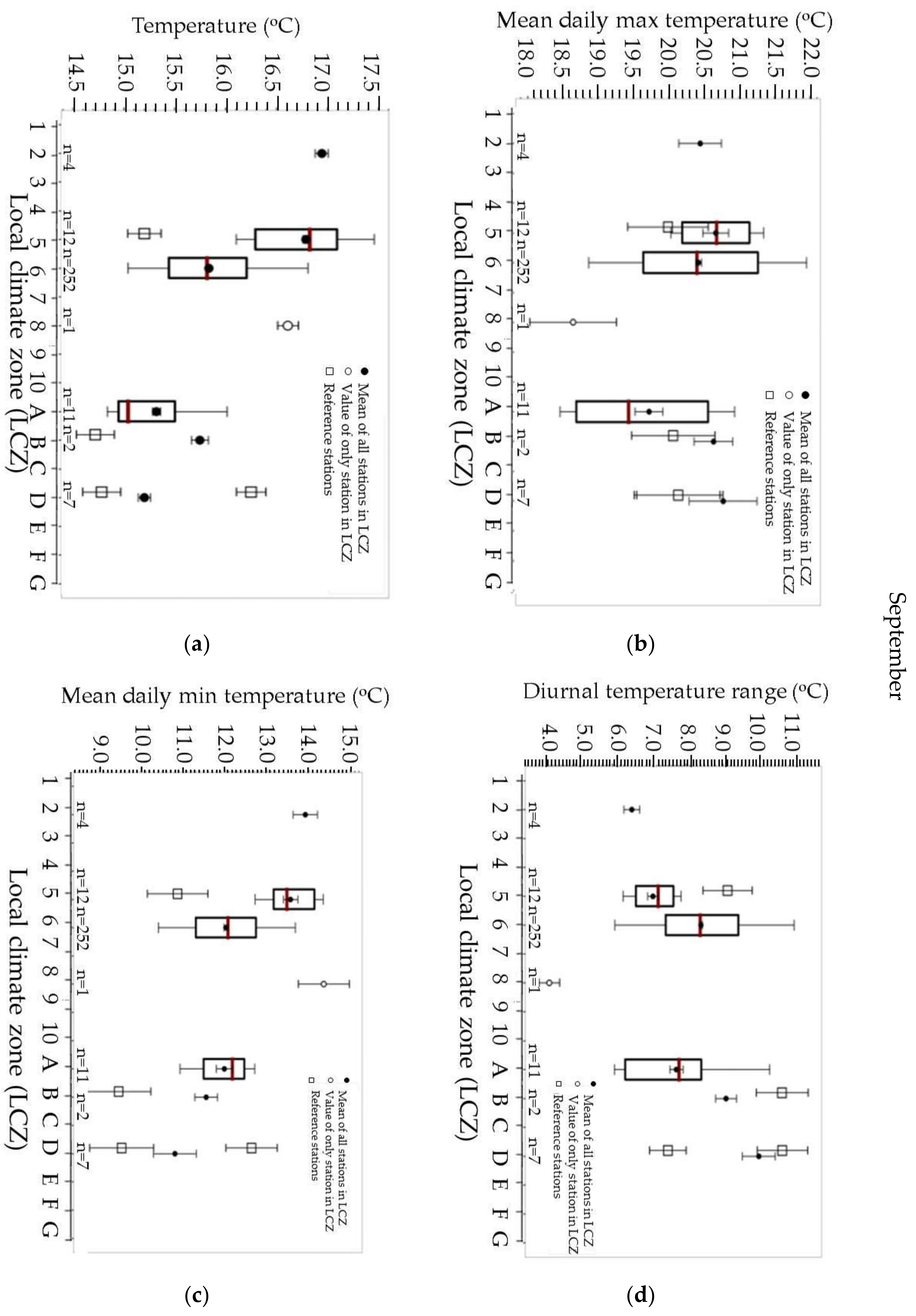
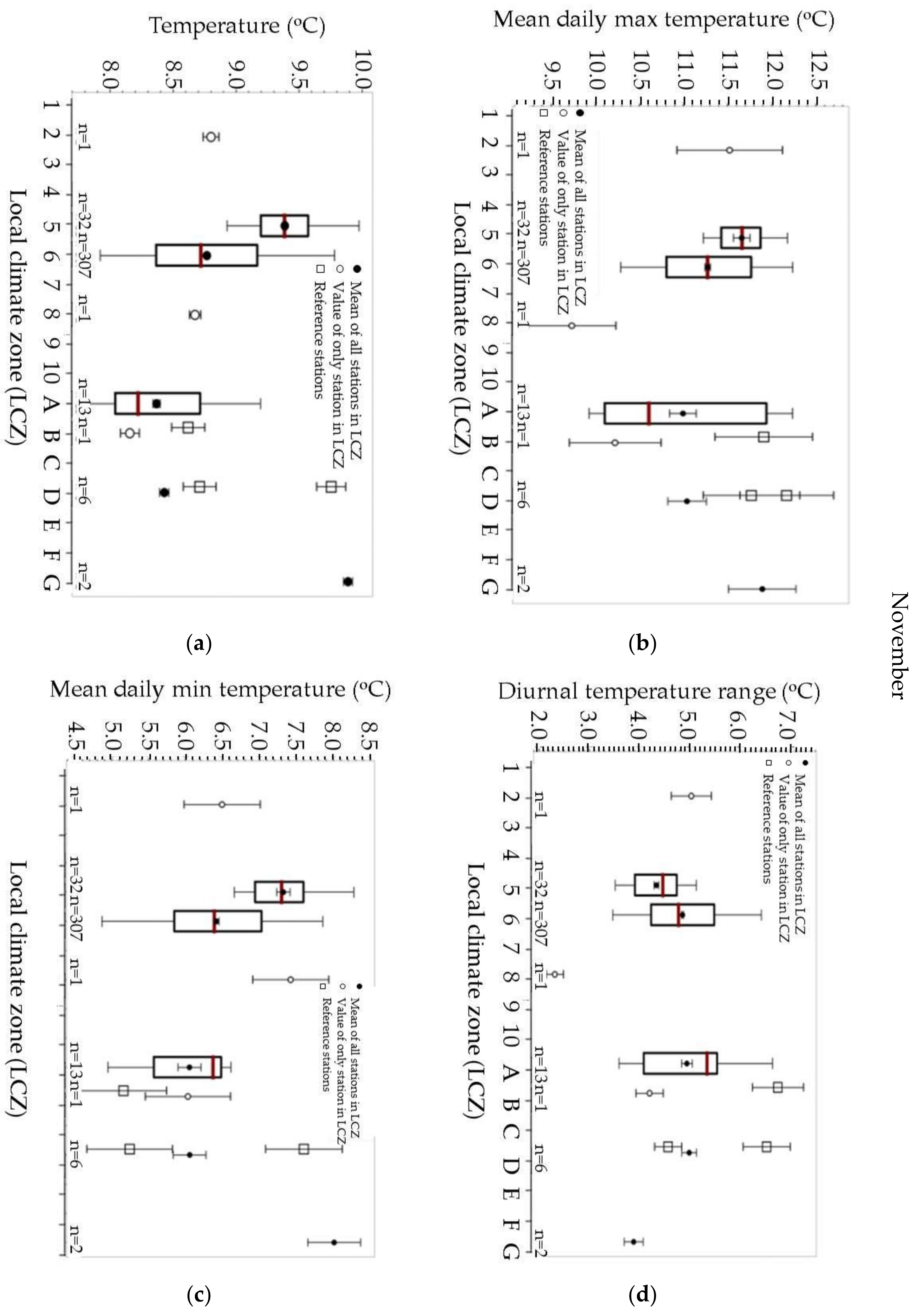
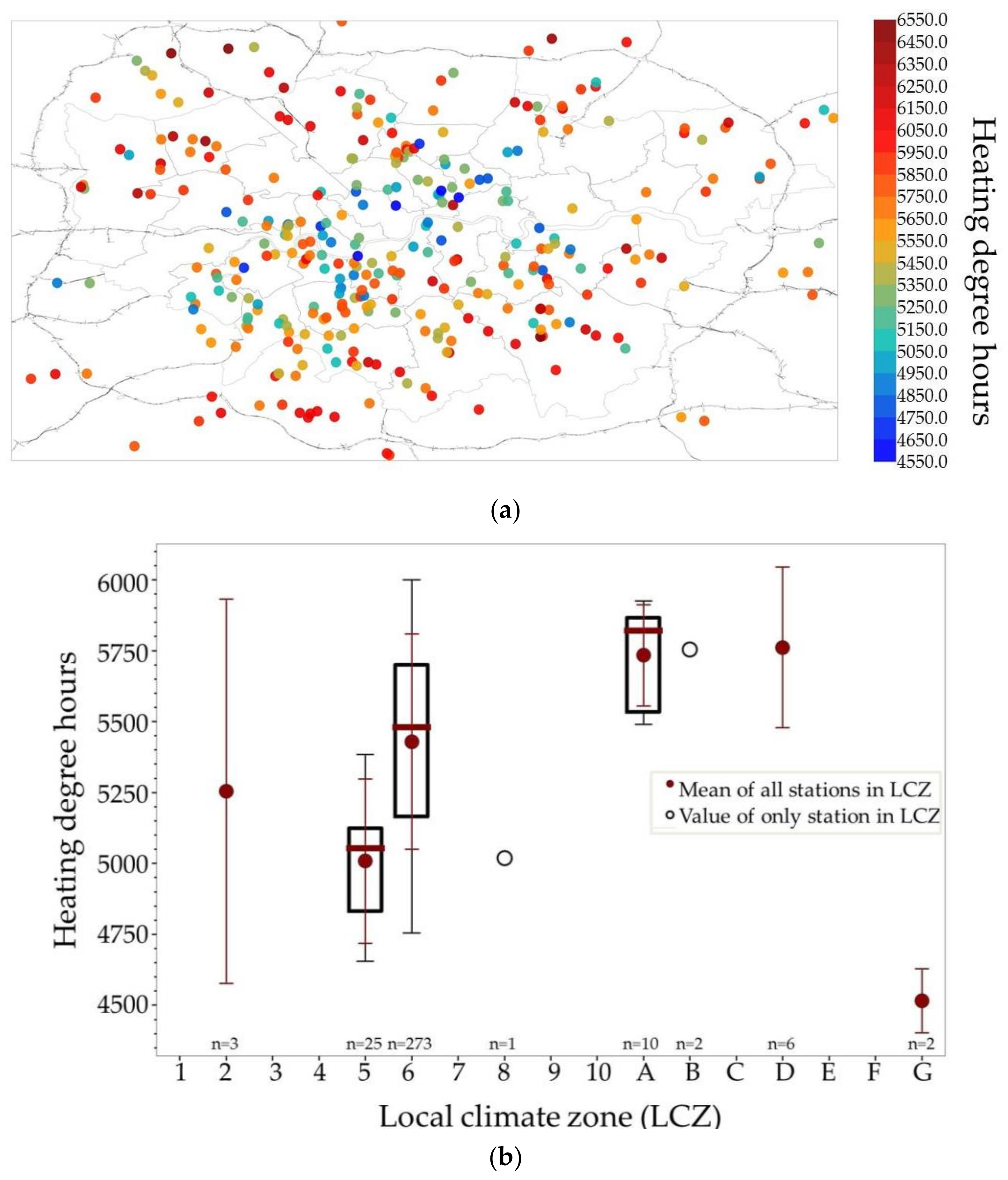
3.2. LCZ Temperature Characteristics

Monthly box plots of mean Tmean, Tmax, Tmin, and DTR in each LCZ are generally consistent with the definition of the characteristics of LCZs. The box plots for July and December are displayed as exemplars for a summer and winter month in Figure 5 and Figure 6, respectively. Box plots are also displayed for LCZs with more than ten stations present. The method of error calculation of the means is shown in Appendix A. The remaining months are displayed in Appendix B, Figure A1, Figure A2 and Figure A3. In general, LCZs associated with more urban landscapes (LCZs 1–10) have a higher mean and minimum temperature than those associated with rural landscapes (LCZs A–G). This is especially prevalent in the summer months. In July, August, and September, LCZ 2 (compact mid-rise) displayed the highest mean temperature. LCZ 2 is the densest urban LCZ present in London and would be expected to have the highest temperatures. Differences in maximum temperature are generally smaller when compared to differences in minimum temperature. This is consistent with the understanding of urban heat islands, as urban areas have a higher thermal capacity so retain more heat during the night than rural areas. Alternatively, during the day, urban areas are often observed to be slightly cooler than rural areas. Because of this, rural LCZs would be expected to have a greater diurnal temperature range than urban LCZs. This is evident in July but is not obvious in other months. Analysis of the average diurnal cycle of each LCZ is shown in Figure 7. It shows a general trend of warmer temperatures in more built-up LCZs, especially at night. In July, maximum temperatures appear comparable for all LCZs, whereas in December there are still large differences between urban and rural in the middle of the day.
Although in many aspects, these results are consistent with the understanding of urban heat islands and the LCZ scheme, inconsistencies between the results and the expected temperature characteristics do exist, especially in cases where there are a low number of stations in an LCZ. One such inconsistency is that in December (Figure 6) and November (Appendix B, Figure A3), LCZ 2 (compact midrise) was cooler than LCZ 5 (open midrise). In the average December diurnal cycle (shown in Figure 7b), LCZ 5 is hotter than LCZ 2 throughout the day, contrary to the thermal definition of these two urban classifications. This is likely related to the small number of stations in LCZ 2 in these months. There was only one qualified station in LCZ 2 in November and three in December. The sample cannot be representative of the entire LCZ and any station taking erroneous readings will play a considerable role in skewing the mean temperature of the LCZ. Therefore, LCZ 2 values are more likely to be erroneous in these months.
Figure 5. Local climate zone (LCZ) temperature characteristics in July 2018: (a) is the mean temperature over the entire month, (b) is the mean daily maximum temperature, (c) is the mean daily minimum temperature, and (d) is the mean diurnal temperature range. LCZs associated with urban landscapes (LCZs 1-10) are on the left side and those associated with rural landscapes (LCZs A–G) are on the right side. n represents the number of valid stations in that LCZ. Filled dots represent the mean of all Netatmo stations in each LCZ, unfilled dots represent the value of the only Netatmo station in an LCZ and squares represent values of reference stations. Box plots are also displayed for LCZs with more than ten stations present. The maroon central line represents the median, the upper and lower bands of the box are the 75th and 25th percentiles and the upper and lower whiskers are the 95th and 5th percentile. The method of error calculation of the means is shown in Appendix A.
Energies 14 05208 g005
Figure 7 shows the mean diurnal temperature cycle for each LCZ. Some unreasonable result appears. For example, LCZ 4 in July (Figure 7a) achieved maximum temperature earlier than others. These occur primarily in LCZs with few stations, which is probably due to the data loss at certain times.
Figure 6. As for Figure 5 but for December 2018.
Energies 14 05208 g006
The reference stations show some temperature consistency with that expected from the LCZ scheme, but it’s clear there is also dependency on the site itself. The ‘London City’ station, which is classed as being in LCZ D, consistently measures higher temperatures than both the other reference station in LCZ D (Northolt) and crowdsourced data. Other than London City, the other stations do show a slight trend of higher mean and minimum temperature in more built-up LCZs. It is noteworthy that in the summer months, crowdsourced temperatures are generally higher than reference temperatures in each LCZ except the ‘London City’ station. This is possible because crowdsourced sensors are heated not only by shortwave radiation, but also by longwave radiation from walls [23]. Interestingly, however, in the winter months, the reference mean temperature and maximum temperature were close to, or greater than, the crowdsourced. These differences between summer and winter may relate to the differences in incoming radiation between summer and winter. In the winter, when there’s less solar radiation, the role of longwave heating of Netatmo stations by nearby walls will be considerably less. Having access to more reference data from stations with more homogeneous surroundings would benefit these comparisons.
Figure 7. The mean diurnal temperature cycle for each LCZ (mean temperature of every station in the relevant LCZ at that hour) for July (a) and December (b). The number of stations in each LCZ is the same as that indicated in Figure 5 for July and Figure 6 for December. LCZs 2, 6, A, and D are highlighted to emphasise differences between LCZs with different forms, and that is common in London.
Energies 14 05208 g007

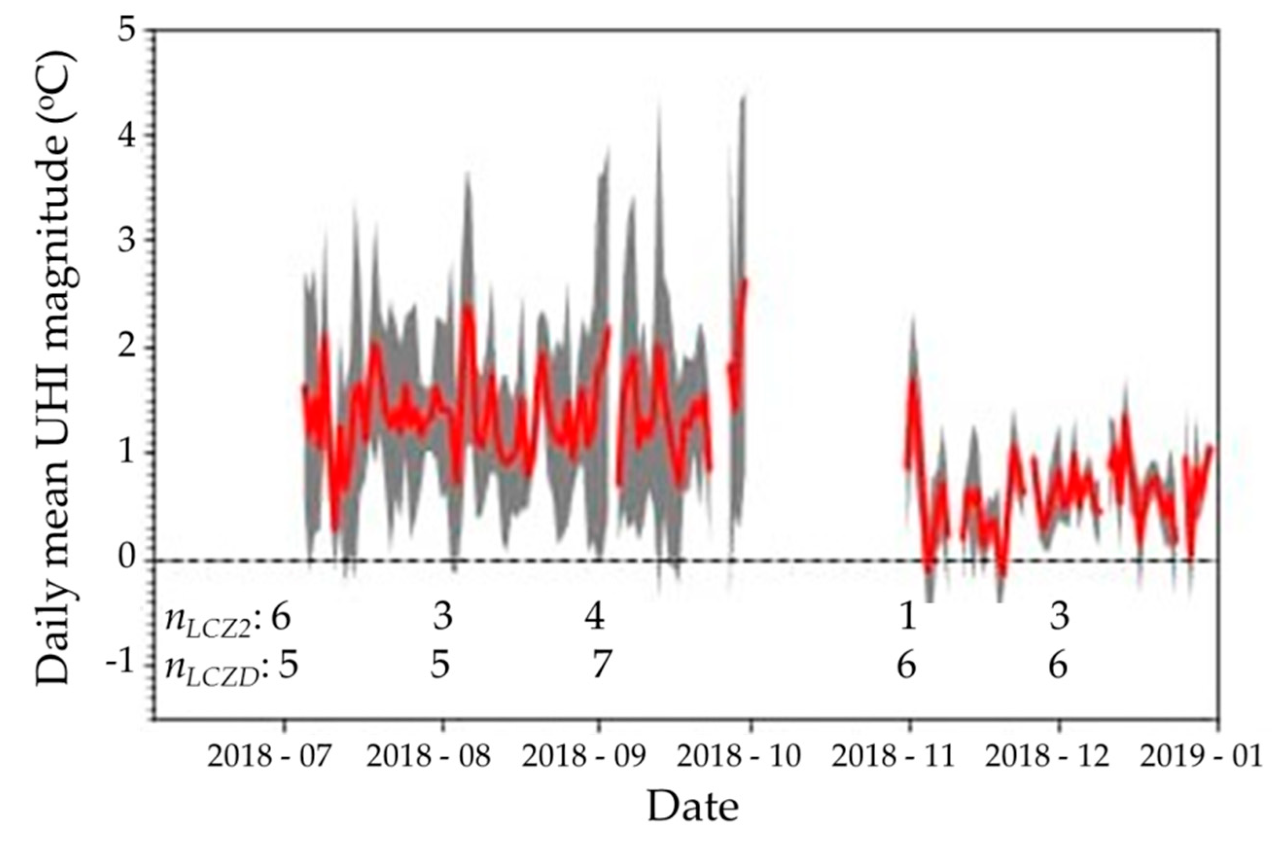
3.3. Urban Heat Island

Over the entire study period, the mean UHI magnitude was 1.07 °C ± 0.03 °C, which is remarkably similar to the average in London from 1901–2006 (1.1 °C) [40]. Jones and Lister found differences in 30-year mean temperatures between the stations in St James’s Park and Rothamsted, noting no significant change in the difference in temperature between these sites over this time. London’s UHI was then quantified by averaging over these 30-year periods. Although the method of data collection and UHI quantification varies greatly from this study, it still shows that the Netatmo estimated mean UHI is in the correct range at the very least. A maximum UHI magnitude of 4.89 °C ± 1.29 °C, was recorded, at midnight on the 30th of September. This is slightly less than that found by Chapman et al. [14] and Watkins et al. [41], who found maximum magnitudes of 5.5 °C and 7 °C, respectively. Again, this is not surprising due to the differences in techniques for UHI classification used in each study. This lack of consensus on UHI quantification is a major issue in UHI research [42] and was a key motivation for the development of the LCZ scheme.
A time series of the daily mean UHI over the study period is displayed in Figure 8. This shows the UHI fluctuating around 1 °C in July, August, and September. In the winter months, the UHI magnitude is noticeably lower, and rarely exceeds 1 °C. This trend of summer and autumn having a stronger UHI is consistent with previous observations of London’s UHI [43]. However, it should also be noted that the number of stations in LCZs 2 and D that passed the QC is variable in different months. It may also impact results. It is possible that a station in LCZ 2 that was systematically measuring high temperatures in the summer, did not pass the QC in the winter months, and therefore did not contribute to UHI calculation in the winter.
Figure 8. The daily mean urban heat island magnitude (defined as TLCZ2–TLCZD), indicated by the red line. nLCZ2 and nLCZD represent the most common number of stations for that month in LCZ 2 and LCZ D, respectively. The filled grey area shows the area between the mean plus one standard deviation and the mean minus one standard deviation.
Energies 14 05208 g008

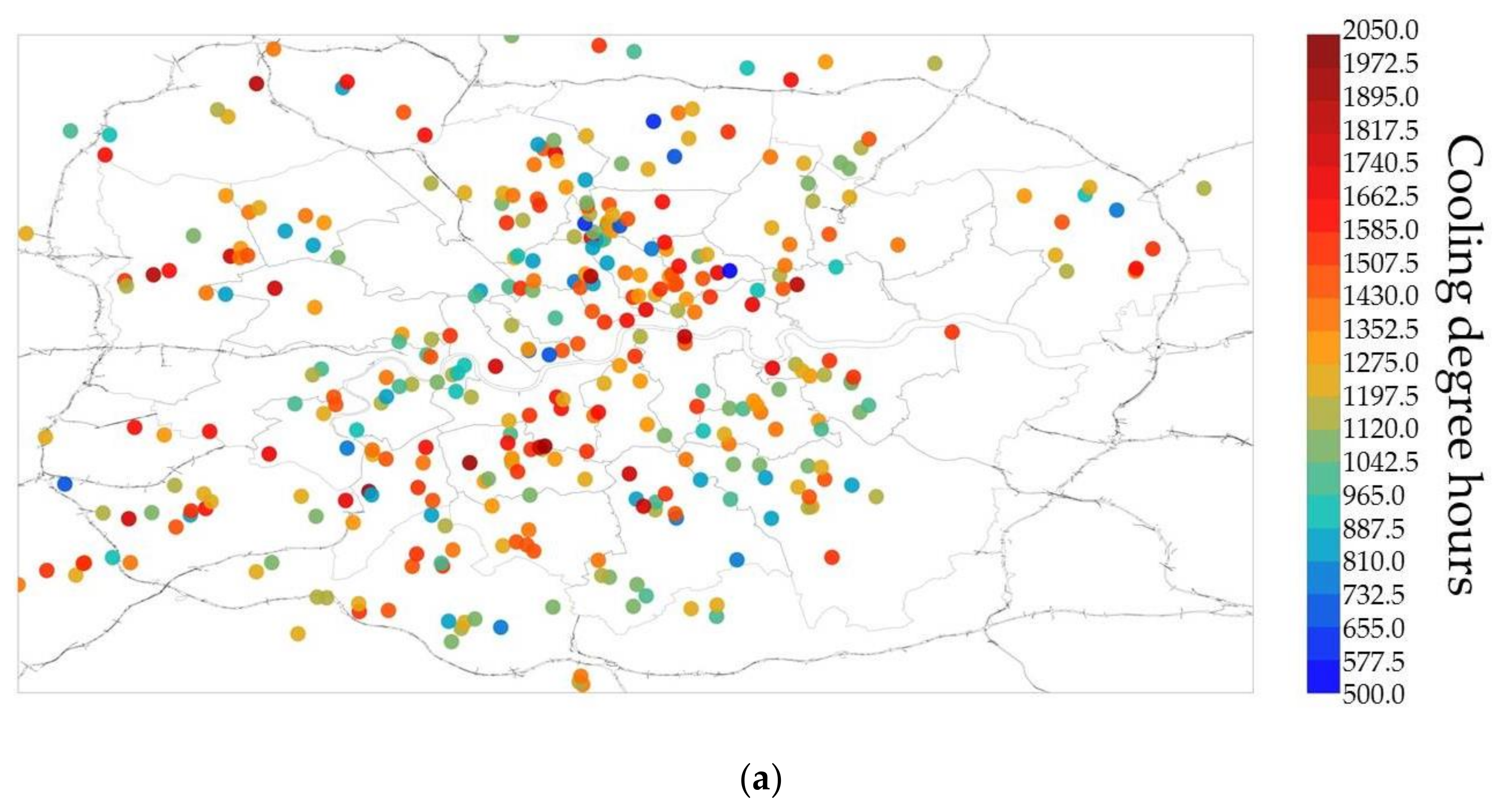
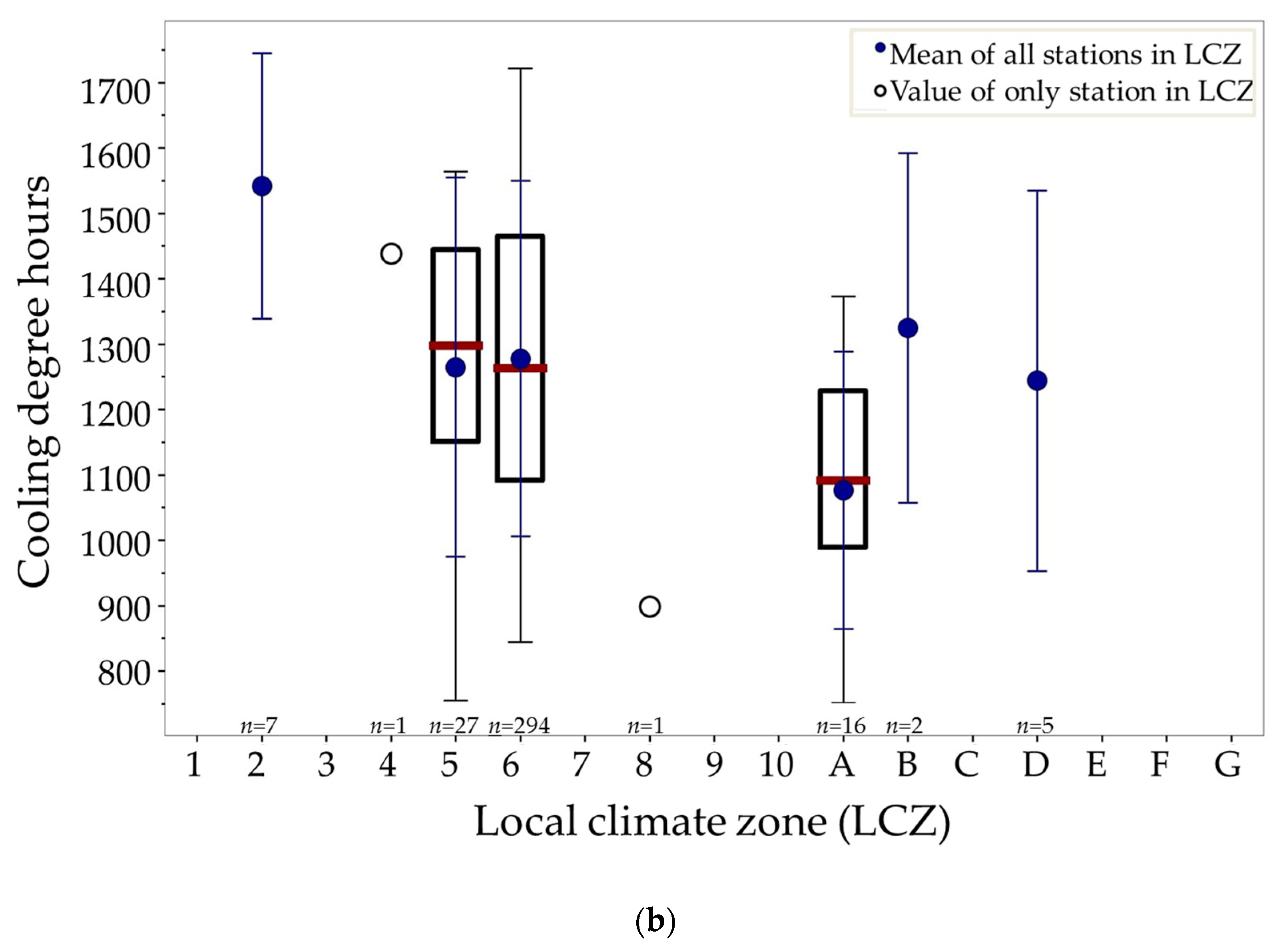
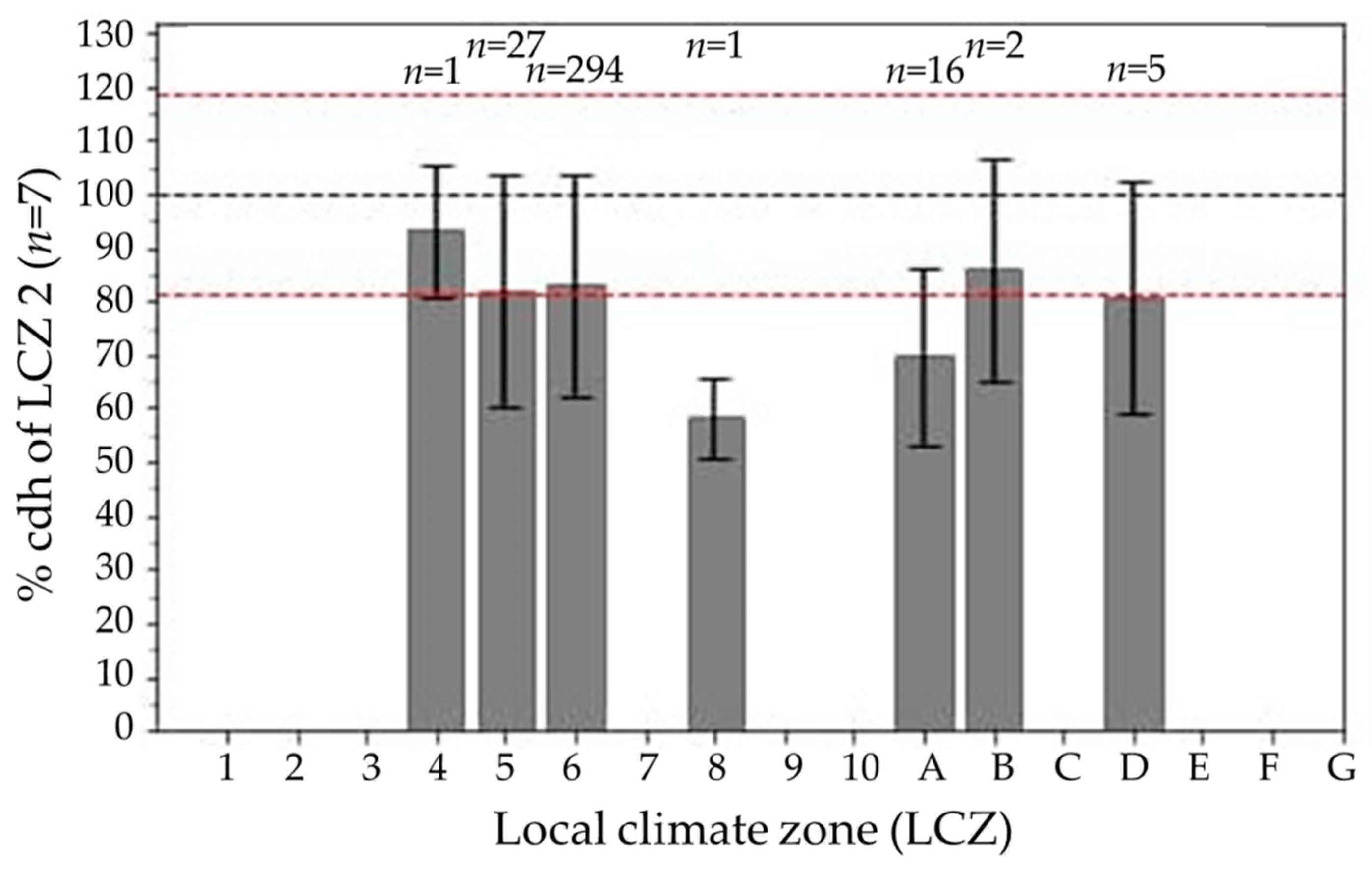
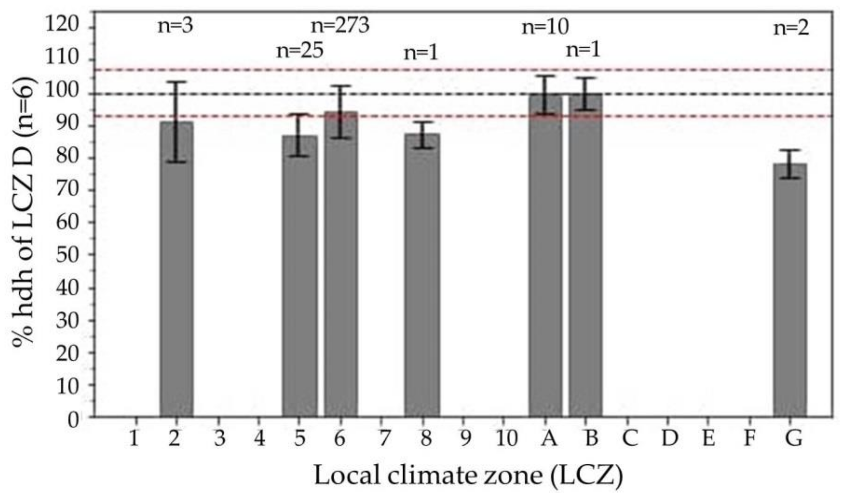
3.4. Building Energy Consumption

Figure 9 shows the building cooling demand in London in July 2018. The general spatial trend of cooling degree hours (CDH) was that CDH is highest in London city centre, with it decreasing further from the centre (Figure 9a). As CDH has a linear relationship with building energy usage for cooling [38], this indicates the highest energy usage in the city centre, with usage decreasing towards the outskirts. The decrease is not uniform in all directions. In addition, variability between stations is high, with some stations directly adjacent to each other measuring very different CDH. After classifying stations into their relevant LCZ and finding the mean CDH in each LCZ (Figure 9b), it’s seen that LCZ 2 (compact midrise) requires the most energy for cooling purposes with a total CDH of 1550. This is to be expected because LCZ 2 is where the geometry, construction materials, and anthropogenic heat release typically lead to the warmest temperatures. LCZ 8 (large low-rise) has the least cooling demand, although there is only one valid station in this LCZ, making the accuracy of this value questionable. Figure 10 shows mean cooling degree hours in July 2018 for each LCZ expressed as a percentage of the mean cooling degree hours of LCZ 2. LCZ A (dense trees) had the second-lowest cooling demand with just 70% of the cooling demand of LCZ 2. Urban LCZs 5 (compact midrise) and 6 (open midrise) and rural LCZs B (scattered trees) and D (low plants) have similar cooling demands, all with between 80% and 85% of the cooling demand of LCZ 2. This is likely due to the similar maximum temperatures between these LCZs (Figure 5b). Temperatures in LCZs 5 and 6 only exceed the CDH base temperature of 22 °C from the late morning to the early evening. Therefore, temperatures during the hottest hours of the day will be the only temperatures included in the CDH calculation. Since the urban-rural temperature differences during the calculation hours are small (as seen in Figure 7), the cooling demands in these LCZs are similar. Overall this suggests that suburban areas have similar cooling demand to many rural landscapes, however, more compact urban environments have significantly higher demand. As LCZs 5 and 6 will be largely residential, this implies that the UHI may not have a great impact on housing cooling demand in London. However, the cooling demand of office buildings, which are more likely to be in LCZ 2, will be significantly affected by the UHI. The finding that rural LCZs B and D have between 80% and 85% of the cooling demand of LCZ 2 is comparable to the findings of previous research.
Figure 9. Building cooling demand in London in July 2018: (a) the spatial distribution of cooling degree hours. Red colours indicate greater cooling demand than blue colours. (b) The mean cooling degree hours of each LCZ. Filled blue dots represent LCZs with more than one station inside; unfilled dots represent LCZs with only one station inside. Errors on the means are one standard deviation. Boxes are plotted for LCZs with more than ten stations within them. The meaning of the bounds and whiskers of the boxes are explained in Figure 5.
Energies 14 05208 g009aEnergies 14 05208 g009b
Figure 10. Mean cooling degree hours in July 2018 for each LCZ expressed as a percentage of the mean cooling degree hours of LCZ 2 ( CDH LCZx CDH LCZ 2 × 100 , where LCZ x is the LCZ to be expressed as a percentage of LCZ 2). n represents the number of stations in each LCZ contributing to the mean. The red dashed line shows the error in the CDH calculation for LCZ 2. Error calculations can be seen in Appendix A.
Energies 14 05208 g010
Figure 11 draws the spatial distribution of heating degree hours (HDH) in December. It shows an inverse trend to that of the July CDH, with less heating demand in the city centre and increasing demand further out. As with Figure 11a, there is high variability in this trend. The LCZ box plot (Figure 11b) shows LCZ 5 has the least heating demand, even less than the more densely urban LCZ 2. The reason for this is ambiguous but may be related to the small number of stations in LCZ 2 (mentioned in Section 2.4. Rural LCZs have a considerably greater heating demand than urban LCZs with mean rural HDH is more than 350 higher than that of any urban LCZ. The differences in heating demand between urban and rural LCZ is clearer than that of cooling demand in July. This is because the greatest LCZ temperature differences are at night when temperatures are more likely to be further below the base temperature. Night temperatures drop in rural stations is further below the base temperature and last longer than in urban stations.
Figure 12 shows the heating demand of each LCZ, expressed as a percentage of the heating demand of LCZ D. It is expressed as a percentage of LCZ D as opposed to LCZ 2 because of the low number of valid stations in LCZ 2 in December. It’s seen that the heating demand of the rural LCZs A and B are identical to that of LCZ D, with all having around 5750 heating degree hours. The remaining, more urban, zones have between 85% and 95% of the heating demand. For example, LCZs 2, 5, and 6 had 91%, 86%, and 95% of the heating demand of LCZ D, respectively.

4. Discussion

In using crowdsourcing and the local climate zone scheme, this study has utilised two techniques that can be considered, relatively speaking, to still be in their infancy. Although both have proven exceedingly useful for producing the results displayed in this paper, the combined use of them has led to several difficulties. Overall, the inter-LCZ analysis of temperature showed many features that would be expected based on the understanding of the urban environment and the definitions of LCZs. However, in some cases, inter-LCZ differences were not consistent, such as LCZ 2 not being the hottest in the winter months (e.g., Figure 6). These inconsistencies almost exclusively arise in LCZs in which there are less than around five stations. It has been noted previously by Napoly et al. that even after a quality check, measurements from a single station should not be trusted. This can also be extended to a small number of stations when carrying out LCZ analysis. Adding to the uncertainty is the fact that in some cases, singular stations can show thermal characteristics consistent with the definition of the LCZ they are classified into. Therefore, it is difficult to know what results can be fully trusted. It may be beneficial to standardise a minimum amount of crowdsourced stations for an LCZ to be analysed. The difficulty with this is that citizen weather stations (CWS), especially in London, are found primarily in suburban areas, meaning these zones have high representation, whereas other LCZs don’t. Once a QC is implemented and stations with heterogeneous surroundings eliminated, this often leaves very few stations in most LCZs. However, as CWS popularity grows over time, this may become less of an issue. The high number of stations located in LCZ 6 does generate a potential area of further research, as it can be investigated whether variability in this LCZ is dependent on the area of London the station is in. This would help determine the validity of the LCZ scheme in London as the temperature variability in LCZ 6 between areas of London could be compared to inter-LCZ variability.
The presence of stations classified in LCZ G (water) raises further concerns about combining the use of Netatmo stations and LCZs. There’s a possibility that these stations could be legitimate and be located on boats on the River Thames. However, it seems more likely that this arises from errors in either the LCZ classification or Netatmo location. It could be that the LCZ map downloaded from the WUDAPT website is not perfectly accurate, or maybe stations located close to the banks of the Thames are classified into LCZ G as the pixel it is within is primarily water. Alternatively, this may arise from inaccuracies in the broadcasted location of these Netatmo stations. Regardless, the presence of stations in LCZ G does raise question marks whether other stations used in this study were classified into LCZs that, in reality, they were not located within. As the methods of urban classification become more refined and detailed, these kinds of errors should be mitigated. Ensuring that Netatmo location is always inputted to a high precision would also improve the applicability of using Netatmo stations for urban climate studies.
Discussed here is just a selection of a wide number of difficulties from using CWS data, coupled with the LCZ scheme, for scientific research. There still seems to be some way to go before CWS data can be used to initialise numerical weather prediction models, as has been suggested previously [21]. As has been mentioned in several cases [14,24]; the scientific use of Netatmo stations would be greatly improved by the stations having more metadata available. In that way, the quality of the data from the station will become clearer. Despite this, there is certainly great potential in the use of these techniques. The unparalleled high spatial density of CWSs provides the potential to unlock a wealth of knowledge of urban climates. In the future, it could be possible that city planners will know what the exact thermal properties of an urban area being developed will be. Then they can know what the characteristics of the building energy usage and heat-related risk to human health will be. The use of crowdsourced data and the LCZ scheme could well contribute to achieving this. Hence, further research into this topic should be carried out.
In London, the UHI may not have a great impact on housing cooling demand. However, the cooling demand of office buildings will be significantly affected by the UHI. The finding that rural LCZs have between 80% and 85% of the cooling demand of urban LCZ is comparable to the findings of previous research. Kolokotroni et al. [5] found that in a typical hot week, a rural office has 84% of the cooling demand of a similar office in urban London. This shows a reasonable degree of coherency between the findings of UHI impact on building energy, despite the methods used to obtain the findings being dramatically different.
Despite winter heating demand having a clearer difference between urban and rural LCZs, percentage differences in summer cooling demand are greater than percentage differences in winter heating demand. These results suggest the reduction in heating by the UHI is less than previous estimates. Watkins et al. [44] found that the annual heating load is 22% less in urban London compared to rural surroundings. This study suggests a reduction of the urban heating load of around 5–15%. This difference may simply be down to the differences in study period time and length.
It should be noted that the magnitude of HDH in December greatly exceeds that of CDH in July. HDH for a single station reached values of 6500, whereas CDH reached only 2000. This shows that even during heatwave conditions, summer cooling demand in London is not as significant as winter heating demand. For both summer cooling and winter heating demand, the standard deviation of the mean is high for all LCZs, suggesting high variability within each LCZ. This variability suggests that building cooling load may not depend only on LCZ. There may be dependence on site-specific parameters such as the amounts of anthropogenic heat release. Alternatively, the variability could be due to certain stations receiving longwave radiation from nearby walls or due to incorrect LCZ classification of certain stations (as discussed above).
Finally, it should be noted that the degree hours approach used in this study is only a proxy to real heating and cooling load for a specific building as this approach only considers the outdoor air temperature. Apart from outdoor air temperature, many other factors contribute to the variability of the building energy consumption in the cities e.g., solar radiation, wind speed and direction, and building features. More advanced building energy simulation tools e.g., EnergyPlus could be used to understand the energy consumption for a specific building located in different parts of the city which will lead to our future research. The datasets collected in this research could serve as a good database for future projects as well.

5. Conclusions

Crowdsourced data from Netatmo personal weather stations has been used to investigate the thermal characteristics and building energy consumption of each local climate zone (LCZ) in London. Data from over 1300 Netatmo stations was collected, from July 2018 to December 2018, which included a summer heatwave period. Each station was classified into an LCZ, using LCZ data obtained from World Urban Database and Access Portal Tools (WUDAPT). As the quality of data from Netatmo stations cannot be known, a quality check, devised by Napoly et al. [23], was implemented. This undoubtedly improved the quality of data used but at the cost of a 50% reduction in data availability.
For the most part, the temperature differences between LCZs are consistent with the definition of LCZs [34], with urban LCZs generally having higher mean temperatures than rural LCZs. Urban LCZs also have a trend of significantly warmer minimum temperatures, especially in the summer months. This is most likely due to the building materials used in urban areas retaining more heat over the nighttime. The urban heat island (UHI) has been defined as the temperature difference between LCZ 2 (compact midrise) and LCZ D (low plants). The mean UHI was found to be 1.07 °C ± 0.03 °C, which is comparable to previous estimations of London’s heat island.
The building cooling demand was analysed in July and heating demand analysed in December, using cooling and heating degree hours (CDH/HDH). The magnitude of the heating degree hours in December far exceeded the magnitude of cooling degree hours in July, despite the heatwave. LCZ 2 had the highest July cooling demand, with a total CDH of 1550. The suburban-related LCZs 5 (open midrise) and 6 (open low-rise) had a similar cooling demand to the rural LCZs B (scattered trees) and D (low plants), with all these zones having between 80% and 85% of the demand of LCZ 2. LCZ A (dense trees) had just 70% of the cooling demand of LCZ 2. In December, rural LCZs had the highest heating demand, with LCZs A, B, and D all having a total HDH of around 5750. Urban LCZs 2, 5, and 6 had 91%, 86%, and 95% of the heating demand of LCZ D, respectively.
Additional refining of the use of crowdsourced weather data is still necessary for its potential to be fully utilised. Implementing a quality check greatly improves data quality but temperature readings from a single/small number of stations still often don’t adhere to the understanding of the urban climate. It is difficult to know what results can be trusted and what can’t. As has been stressed before, improved metadata of Netatmo stations would help address this issue. This study highlights the potential of crowdsourced data in distinguishing differences in building energy usage between LCZs, however, it has also accentuated some of the issues in using it. Once these issues are addressed, crowdsourced data may well become key to improving understanding of the urban climate and applying this understanding to city planning.

Author Contributions

Conceptualization, Z.L.; methodology, K.B.; software, K.B.; resources, Z.L.; data curation, K.B.; writing—original draft preparation, K.B.; writing—review and editing, X.W. and Z.L.; visualization, K.B. and X.W; supervision, Z.L. All authors have read and agreed to the published version of the manuscript.

Funding

This research was funded by UROP UG research at the University of Reading, GuangDong Basic and Applied Basic Research Foundation with Grant 2020A1515110763, and the Innovation of Science and Technology Commission of Shenzhen Municipality Ministry with Grants of JCYJ 20180305180905450.

Institutional Review Board Statement

Not applicable.

Informed Consent Statement

Not applicable.

Data Availability Statement

Netatmo weather map is obtained from https://weathermap.netatmo.com/ (accessed on 29 January 2019). London LCZ map was downloaded from the WUDAPT website: http://www.wudapt.org/ (accessed on 29 January 2019).

Acknowledgments

The authors would like to acknowledge Fred Meier for his guidance on the quality check of Netatmo data.

Conflicts of Interest

The authors declare no conflict of interest. The funders had no role in the design of the study; in the collection, analyses, or interpretation of data; in the writing of the manuscript, or in the decision to publish the results.

Appendix A. Error Calculations

Appendix A.1. Temperature

To calculate the errors shown in the inter-LCZ temperature plots (Figure 4 and Figure 5), the standard error of the mean was calculated for every station, for each variable (mean temperature, minimum temperature, maximum temperature, and DTR):
σ LCZ = SD n
where SD is the standard deviation and n is the sample size.
For LCZ with only one station, and for reference stations, this standard error was presented on the plot. For LCZs with more than one station within them, these individual errors were then combined to find the error in the LCZ ( σ LCZ ) using the following expression:
σ LCZ = i = 1 i = n σ i 2 n
where i is the standard error of an individual station and n is the number of valid stations in an LCZ. Note σ can represent the error in any of the aforementioned variables (mean temperature, minimum temperature, maximum temperature and DTR).

Appendix A.2. Cooling/Heating Degree Hours Percentages

The errors on the cooling degree hours for each LCZ expressed as a percentage of LCZ 2 (as shown in Figure 8) are calculated by combining the errors on the cooling degree hours of the two LCZs:
σ P LCZ   i   = P LCZ   i × ( σ CDH LCZ   i CDH LCZ   i ) 2 + σ CDH LCZ   2 CDH LCZ   2 2
where P LCZ   i is the percentage of the LCZ’s CDH to LCZ 2′s CDH. σ CDH LCZ   i is the error in the LCZs CDH calculation and σ CDH LCZ   2 is the error in LCZ 2′s CDH calculation (i.e., one standard deviation from the mean). CDH LCZ   i is the CDH of the LCZ and CDH LCZ   2 is the CDH of LCZ 2.
The errors on the heating degree hours for each LCZ expressed as a percentage of LCZ D (as shown in Figure 10) is calculated the same way but replacing CDH with HDH and LCZ 2 with LCZ D.

Appendix B. Box Plots of Thermal Properties for August, September and November

Figure A1. Local climate zone (LCZ) temperature characteristics in August 2018: (a) is the mean temperature over the entire month, (b) is the mean daily maximum temperature, (c) is the mean daily minimum temperature, and (d) is the mean diurnal temperature range. LCZs associated with urban landscapes (LCZs 1-10) are on the left side and those associated with rural landscapes (LCZs A–G) are on the right side. n represents the number of valid stations in that LCZ. Filled dots represent the mean of all Netatmo stations in each LCZ, unfilled dots represent the value of the only Netatmo station in an LCZ and squares represent values of reference stations. Box plots are also displayed for LCZs with more than ten stations present. The maroon central line represents the median, the upper and lower bands of the box are the 75th and 25th percentiles and the upper and lower whiskers are the 95th and 5th percentile. The method of error calculation of the means is shown in Appendix A.
Energies 14 05208 g0a1
Figure A2. Local climate zone (LCZ) temperature characteristics in September 2018: (a) is the mean temperature over the entire month, (b) is the mean daily maximum temperature, (c) is the mean daily minimum temperature, and (d) is the mean diurnal temperature range. LCZs associated with urban landscapes (LCZs 1-10) are on the left side and those associated with rural landscapes (LCZs A–G) are on the right side. n represents the number of valid stations in that LCZ. Filled dots represent the mean of all Netatmo stations in each LCZ, unfilled dots represent the value of the only Netatmo station in an LCZ and squares represent values of reference stations. Box plots are also displayed for LCZs with more than ten stations present. The maroon central line represents the median, the upper and lower bands of the box are the 75th and 25th percentiles and the upper and lower whiskers are the 95th and 5th percentile. The method of error calculation of the means is shown in Appendix A.
Energies 14 05208 g0a2
Figure A3. Local climate zone (LCZ) temperature characteristics in November 2018: (a) is the mean temperature over the entire month, (b) is the mean daily maximum temperature, (c) is the mean daily minimum temperature, and (d) is the mean diurnal temperature range. LCZs associated with urban landscapes (LCZs 1-10) are on the left side and those associated with rural landscapes (LCZs A–G) are on the right side. n represents the number of valid stations in that LCZ. Filled dots represent the mean of all Netatmo stations in each LCZ, unfilled dots represent the value of the only Netatmo station in an LCZ and squares represent values of reference stations. Box plots are also displayed for LCZs with more than ten stations present. The maroon central line represents the median, the upper and lower bands of the box are the 75th and 25th percentiles and the upper and lower whiskers are the 95th and 5th percentile. The method of error calculation of the means is shown in Appendix A.
Energies 14 05208 g0a3

References

  1. Wei, Y.; Zhang, X.; Shi, Y.; Xia, L.; Pan, S.; Wu, J.; Han, M.; Zhao, X. A review of data-driven approaches for prediction and classification of building energy consumption. Renew. Sustain. Energy Rev. 2018, 82, 1027–1047. [Google Scholar] [CrossRef]
  2. Yang, L.; Yan, H.; Lam, J.C. Thermal comfort and building energy consumption implications—A review. Appl. Energy 2014, 115, 164–173. [Google Scholar] [CrossRef]
  3. Li, X.; Zhou, Y.; Yu, S.; Jia, G.; Li, H.; Li, W. Urban heat island impacts on building energy consumption: A review of approaches and findings. Energy 2019, 174, 407–419. [Google Scholar] [CrossRef]
  4. Santamouris, M.; Papanikolaou, N.; Livada, I.; Koronakis, I.; Georgakis, C.; Argiriou, A.; Assimakopoulos, D. On the impact of urban climate on the energy consumption of buildings. Sol. Energy 2001, 70, 201–216. [Google Scholar] [CrossRef]
  5. Kolokotroni, M.; Giannitsaris, I.; Watkins, R. The effect of the London urban heat island on building summer cooling demand and night ventilation strategies. Sol. Energy 2006, 80, 383–392. [Google Scholar] [CrossRef]
  6. Kolokotroni, M.; Zhang, Y.; Giridharan, R. Heating and cooling degree day prediction within the London urban heat island area. Build. Serv. Eng. Res. Technol. 2009, 30, 183–202. [Google Scholar] [CrossRef]
  7. Xie, X.; Sahin, O.; Luo, Z.; Yao, R. Impact of neighbourhood-scale climate characteristics on building heating demand and night ventilation cooling potential. Renew. Energy 2020, 150, 943–956. [Google Scholar] [CrossRef]
  8. Lowe, S.A. An energy and mortality impact assessment of the urban heat island in the US. Environ. Impact Assess. Rev. 2016, 56, 139–144. [Google Scholar] [CrossRef]
  9. Shi, L.; Luo, Z.; Matthews, W.; Wang, Z.; Li, Y.; Liu, J. Impacts of urban microclimate on summertime sensible and latent energy demand for cooling in residential buildings of Hong Kong. Energy 2019, 189, 116208. [Google Scholar] [CrossRef]
  10. Akbari, H.; Davis, S.; Huang, J.; Dorsano, S.; Winnett, S. Cooling Our Communities: A Guidebook on Tree Planting and Light-Colored Surfacing; Lawrence Berkeley Lab.: Berkeley, CA, USA, 1992. [Google Scholar]
  11. Santamouris, M.; Cartalis, C.; Synnefa, A.; Kolokotsa, D. On the impact of urban heat island and global warming on the power demand and electricity consumption of buildings—A review. Energy Build. 2015, 98, 119–124. [Google Scholar] [CrossRef]
  12. Spinoni, J.; Vogt, J.V.; Barbosa, P.; Dosio, A.; McCormick, N.; Bigano, A.; Füssel, H.M. Changes of heating and cooling degree-days in Europe from 1981 to 2100. Int. J. Climatol. 2018, 38, e191–e208. [Google Scholar] [CrossRef]
  13. Guattari, C.; Evangelisti, L.; Balaras, C.A. On the assessment of urban heat island phenomenon and its effects on building energy performance: A case study of Rome (Italy). Energy Build. 2018, 158, 605–615. [Google Scholar] [CrossRef]
  14. Chapman, L.; Bell, C.; Bell, S. Can the crowdsourcing data paradigm take atmospheric science to a new level? A case study of the urban heat island of London quantified using Netatmo weather stations. Int. J. Climatol. 2017, 37, 3597–3605. [Google Scholar] [CrossRef]
  15. Muller, C.; Chapman, L.; Johnston, S.; Kidd, C.; Illingworth, S.; Foody, G.; Overeem, A.; Leigh, R. Crowdsourcing for climate and atmospheric sciences: Current status and future potential. Int. J. Climatol. 2015, 35, 3185–3203. [Google Scholar] [CrossRef] [Green Version]
  16. Hammerberg, K.; Brousse, O.; Martilli, A.; Mahdavi, A. Implications of employing detailed urban canopy parameters for mesoscale climate modelling: A comparison between WUDAPT and GIS databases over Vienna, Austria. Int. J. Climatol. 2018, 38, e1241–e1257. [Google Scholar] [CrossRef] [Green Version]
  17. Overeem, A.; Robinson, J.R.; Leijnse, H.; Steeneveld, G.-J.; Horn, B.P.; Uijlenhoet, R. Crowdsourcing urban air temperatures from smartphone battery temperatures. Geophys. Res. Lett. 2013, 40, 4081–4085. [Google Scholar] [CrossRef]
  18. Droste, A.M.; Pape, J.J.; Overeem, A.; Leijnse, H.; Uijlenhoet, R. Crowdsourcing urban air temperatures through smartphone battery temperatures in São Paulo, Brazil. J. Atmos. Ocean. Technol. 2017, 34, 1853–1866. [Google Scholar] [CrossRef]
  19. Muller, C.L. Mapping snow depth across the West Midlands using social media-generated data. Weather 2013, 68, 82. [Google Scholar] [CrossRef]
  20. Bell, S.; Dan, C.; Bastin, L. How good are citizen weather stations? Addressing a biased opinion. Weather 2015, 70, 75–84. [Google Scholar] [CrossRef] [Green Version]
  21. Bell, S.; Cornford, D.; Bastin, L. The state of automated amateur weather observations. Weather 2013, 68, 36–41. [Google Scholar] [CrossRef]
  22. Fenner, D.; Meier, F.; Bechtel, B.; Otto, M.; Scherer, D. Intra and inter ‘local climate zone’ variability of air temperature as observed by crowdsourced citizen weather stations in Berlin, Germany. Meteorol. Z. 2017, 26, 525–547. [Google Scholar] [CrossRef]
  23. Napoly, A.; Grassmann, T.; Meier, F.; Fenner, D. Development and application of a statistically-based quality control for crowdsourced air temperature data. Front. Earth Sci. 2018, 6, 118. [Google Scholar] [CrossRef] [Green Version]
  24. Meier, F.; Fenner, D.; Grassmann, T.; Otto, M.; Scherer, D. Crowdsourcing air temperature from citizen weather stations for urban climate research. Urban Clim. 2017, 19, 170–191. [Google Scholar] [CrossRef]
  25. UK Office of National Statistics, 2018: Estimates of the Population for the UK, England and Wales, Scotland and Northern Ireland, Mid-2017. Available online: https://www.ons.gov.uk/peoplepopulationandcommunity/populationandmigration/populationestimates/datasets/populationestimatesforukenglandandwalesscotlandandnorthernireland. (accessed on 28 January 2019).
  26. Kottek, M.; Grieser, J.; Beck, C.; Rudolf, B.; Rubel, F. World map of the Köppen-Geiger climate classification updated. Meteorol. Z. 2006, 15, 259–263. [Google Scholar] [CrossRef]
  27. UK Met Office, 2019: 2018 Weather Summaries. Available online: https://www.metoffice.gov.uk/climate/uk/summaries/2018. (accessed on 28 January 2019).
  28. Zuo, J.; Pullen, S.; Palmer, J.; Bennetts, H.; Chileshe, N.; Ma, T. Impacts of heat waves and corresponding measures: A review. J. Clean. Prod. 2015, 92, 1–12. [Google Scholar] [CrossRef]
  29. Weather Underground, 2019: Personal Weather Station Network. Available online: https://www.wunderground.com/weatherstation/overview.asp. (accessed on 29 January 2019).
  30. UK Met Office, 2012: Met Office Integrated Data Archive System (MIDAS) Land and Marine Surface Stations Data (1853-Current). Available online: http://catalogue.ceda.ac.uk/uuid/220a65615218d5c9cc9e4785a3234bd0. (accessed on 1 February 2019).
  31. UK Met Office, 2006: MIDAS: UK Hourly Weather Observation Data. Available online: http://catalogue.ceda.ac.uk/uuid/916ac4bbc46f7685ae9a5e10451bae7c. (accessed on 1 February 2019).
  32. UK Met Office, 2010: National Meteorological Library and Archive Fact sheet 17—Weather Observations Over Land: Observations. Available online: https://www.metoffice.gov.uk/binaries/content/assets/mohippo/pdf/k/5/fact_sheet_no._17.pdf. (accessed on 29 January 2019).
  33. Bechtel, B.; Demuzere, M.; Sismanidis, P.; Fenner, D.; Brousse, O.; Beck, C.; Van Coillie, F.; Conrad, O.; Keramitsoglou, I.; Middel, A.; et al. Quality of crowdsourced data on urban morphology—The human influence experiment (HUMINEX). Urban Sci. 2017, 1, 15. [Google Scholar] [CrossRef] [Green Version]
  34. Stewart, I.D.; Oke, T.R. Local climate zones for urban temperature studies. Bull. Am. Meteorol. Soc. 2012, 93, 1879–1900. [Google Scholar] [CrossRef]
  35. Ching, J.; Mills, G.; Bechtel, B.; See, L.; Feddema, J.; Wang, X.; Ren, C.; Brousse, O.; Martilli, A.; Neophytou, M.; et al. WUDAPT: An urban weather, climate, and environmental modeling infrastructure for the anthropocene. Bull. Am. Meteorol. Soc. 2018, 99, 1907–1924. [Google Scholar] [CrossRef] [Green Version]
  36. Bechtel, B.; Daneke, C. Classification of local climate zones based on multiple earth observation data. IEEE J. Sel. Top. Appl. Earth Obs. Remote Sens. 2012, 5, 1191–1202. [Google Scholar] [CrossRef]
  37. Bechtel, B.; Alexander, P.J.; Böhner, J.; Ching, J.; Conrad, O.; Feddema, J.; Mills, G.; See, L.; Stewart, I. Mapping local climate zones for a worldwide database of the form and function of cities. ISPRS Int. J. Geo-Inf. 2015, 4, 199–219. [Google Scholar] [CrossRef] [Green Version]
  38. Day, T. Degree-days: Theory and application. Chart. Inst. Build. Serv. Eng. Lond. 2006, 106, 60–81. [Google Scholar]
  39. Azevedo, J.A.; Chapman, L.; Muller, C.L. Critique and suggested modifications of the degree days methodology to enable long-term electricity consumption assessments: A case study in Birmingham, UK. Meteorol. Appl. 2015, 22, 789–796. [Google Scholar] [CrossRef]
  40. Jones, P.D.; Lister, D.H. The urban heat island in Central London and urban-related warming trends in Central London since 1900. Weather 2009, 64, 323–327. [Google Scholar] [CrossRef]
  41. Watkins, R.; Palmer, J.; Kolokotroni, M.; Littlefair, P. The London Heat Island: Results from summertime monitoring. Build. Serv. Eng. Res. Technol. 2002, 23, 97–106. [Google Scholar] [CrossRef]
  42. Stewart, I.D. A systematic review and scientific critique of methodology in modern urban heat island literature. Int. J. Climatol. 2011, 31, 200–217. [Google Scholar] [CrossRef]
  43. Lee, D. Rural atmospheric stability and the intensity of London’s heat island. Weather 1975, 30, 102–109. [Google Scholar] [CrossRef]
  44. Watkins, R.; Palmer, J.; Kolokotroni, M.; Littlefair, P. The balance of the annual heating and cooling demand within the London urban heat island. Build. Serv. Eng. Res. Technol. 2002, 23, 207–213. [Google Scholar] [CrossRef]
Figure 11. Building heating demand in London in December 2018: (a) the spatial distribution of heating degree hours. Red colours indicate greater heating demand than blue colours. (b) the mean heating degree hours of each LCZ. Filled red dots represent LCZs with more than one station inside, unfilled dots represent LCZs with only one station inside. Errors on the means are one standard deviation. Boxes are plotted for LCZs with more than ten stations within them. The meaning of the bounds and whiskers of the boxes are explained in Figure 5.
Energies 14 05208 g011
Figure 12. Mean heating degree hours in December 2018 for each LCZ, expressed as a percentage of the mean heating degree hours of LCZ D ( HDH LCZx HDH LCZD × 100 , where LCZ x is the LCZ to be expressed as a percentage of LCZ D). n represents the number of stations in each LCZ contributing to the mean. The red dashed line shows the error in the HDH calculation for LCZ D. Error calculations can be seen in Appendix A.
Energies 14 05208 g012
Publisher’s Note: MDPI stays neutral with regard to jurisdictional claims in published maps and institutional affiliations.

