Article

Central Bulge Ferrite Core for Efficient Wireless Power Transfer

1
School of Electrical and Electronic Engineering, Shandong University of Technology, Zibo 255000, China
2
School of New Energy, Harbin Institute of Technology at Weihai, Weihai 264200, China
3
School of Information and Control Engineering, Qingdao University of Technology, Qingdao 266525, China
*
Author to whom correspondence should be addressed.
Energies 2021, 14(16), 5111; https://doi.org/10.3390/en14165111
Submission received: 8 July 2021 / Revised: 8 August 2021 / Accepted: 16 August 2021 / Published: 19 August 2021

Abstract

:
To improve the efficiency of the wireless power transfer (WPT) system without increasing the system size, a central bulge ferrite core with a novel configuration is proposed. The mutual inductance between magnetic coupling structures is able to increase obviously, which is approved by eigenfunction expansion method. In this paper, the mathematical models of the planar core and the central bulge core are established, respectively, as two types of the mutual inductance are calculated in same condition. The structure parameters of the central bulge ferrite core are further optimized by Maxwell magnetic field simulation. Experiments are conducted to compare the WPT efficiency of two types of ferrite cores in improving the efficiency of WPT system, in which the influence of transmission distance, lateral misalignment, and load variation are taken into account. The results show that central bulge ferrite core has better performance in WPT efficiency than the planar one, even in the case of long power transfer distance and lateral misalignment.

1. Introduction

With the recent development of electrification, the wireless power transmission has been increasingly used in electric vehicles chargers, biomedical devices, environmental monitoring technology, and robotic systems for the advantages of safety, flexibility, and convenient maintenance [1,2,3,4,5,6]. The wireless power transfer (WPT) system via inductive coupling has been widely used to replace electromagnetic radiation system due to lower power loss and more environmentally friendly [7,8]. However, the efficiency of two-coil system based on the maximum power transfer principle has an inherent limitation that cannot exceed 50% [9,10]. Therefore, how to improve power transmission efficiency has become a key challenge for WPT systems [11].
Increasing the size of inductive coupling coils can enhance the magnetic field to improve transmission efficiency [12]. In recent years, intensive research has been conducted to improve the magnetic coupling relationship by magnetic coupling structure design, and many new types of coils have been proposed [13,14,15]. The WPT systems with more than three coils between the primary and secondary side have the advantages of high coupling coefficient, long transmission distance, and wide operating frequency range [16], which makes multi-coil structure an effective way to improve the power transfer efficiency of WPT system. In [10], a novel U-coil WPT system is developed to improve the transmission efficiency, and it ensures the cleanliness of the space along the transfer direction. The influence of magnetic coupling of nonadjacent resonators on the optimal frequency is investigated to provide a feasible method for the following research of WPT system resonators based on Domino form [17]. However, the increasing number of coils could improve system efficiency, but also expand the system size, which becomes an infeasible solution in some actual conditions where the space is limited. Changing the system’s circuit topology and control strategy become two alternative methods [18,19], but they may often lead to sophisticated control circuit with enormous calculation burden.
To improve the weak coupling magnetic field of the separate coils, adding square and circular planar ferrite core can make a better balance between power transfer efficiency and system size [20,21]. To the further improvement of transfer efficiency, many research groups begin to explore new core structures. In [22], the scheme of replacing the traditional circular planar core with magnetic strips is designed and optimized, which can reduce the system size and weight without sacrificing the transfer efficiency. A new structure of circular and rod cores is proposed in [23] to achieve a better misalignment tolerance and lower loss, but analytic calculation of magnetic field for the special-shaped cores is not included in this paper. In [24], an ameliorated cylindrical core is proposed to weaken the demagnetization factor and improve power transmission efficiency, while this change is non-applicable to the planar cores.
Inspired by the works in [23,24], a central bulge ferrite core is proposed in this paper to increase power transfer efficiency while controlling the system size. In addition, the analytical calculation methods of magnetic field and mutual inductance for special-shaped core are provided. The rest of this paper is structured as follows. In Section 2, the relationship between transmission efficiency and mutual inductance is calculated, then the magnetic field and mutual inductance are computed by mathematical models of the two types of cores. In Section 3, considering the original constraints of the system, the optimization of the proposed core is conducted. In Section 4 and Section 5, the optimized central bulge ferrite core is verified by simulation and experiments. Finally, conclusions are drawn in Section 6.

2. Efficiency Analysis for the Planar Core and the Central Bulge Ferrite Cores

In this section, power transfer efficiency analysis consists of two steps. The influence of mutual inductance on transmission efficiency is investigated in Section 2.1. Then the analytical calculation of mutual inductance and magnetic field for two cores is completed in Section 2.2, which also provides a feasible method to calculate the magnetic field for special-shaped cores.

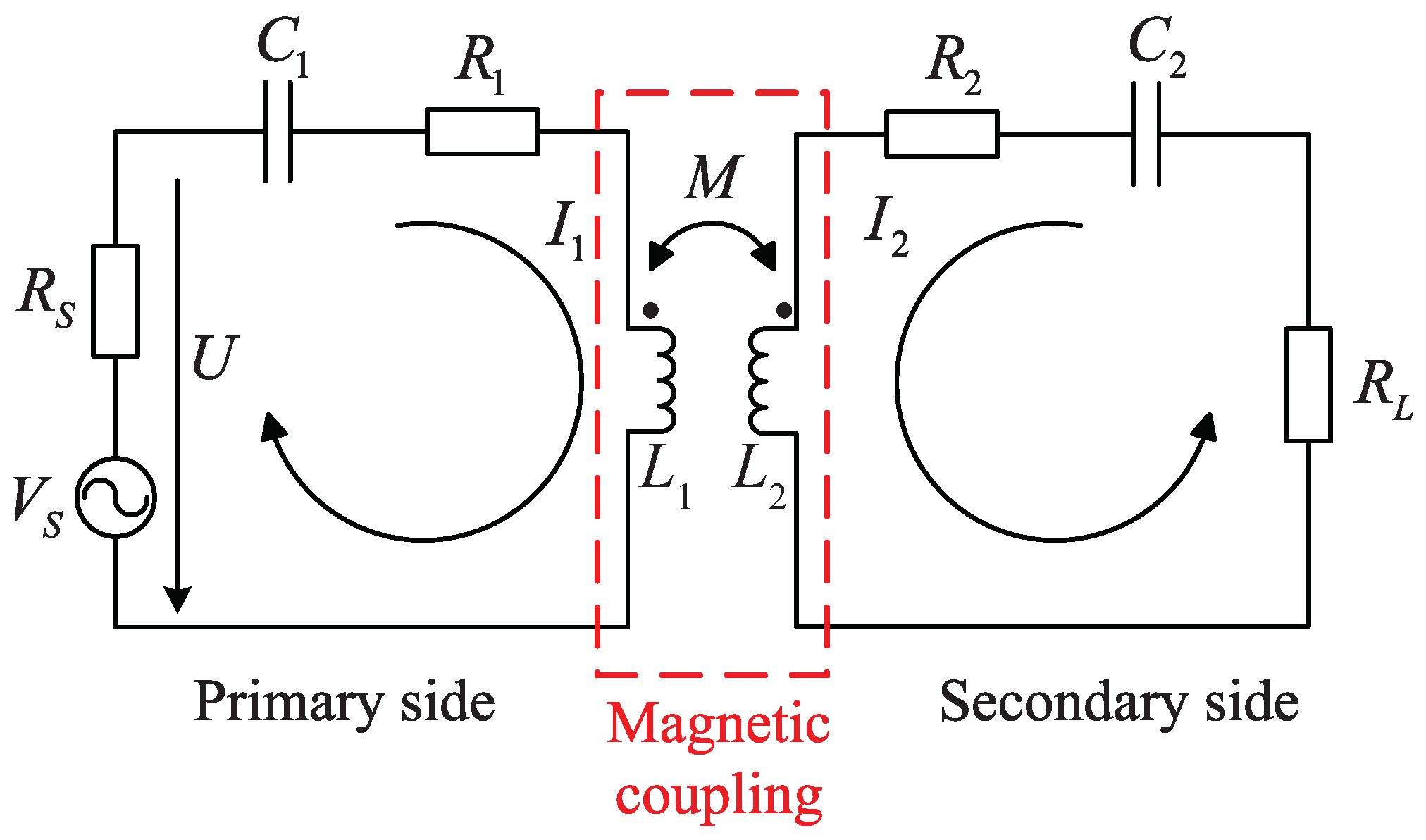
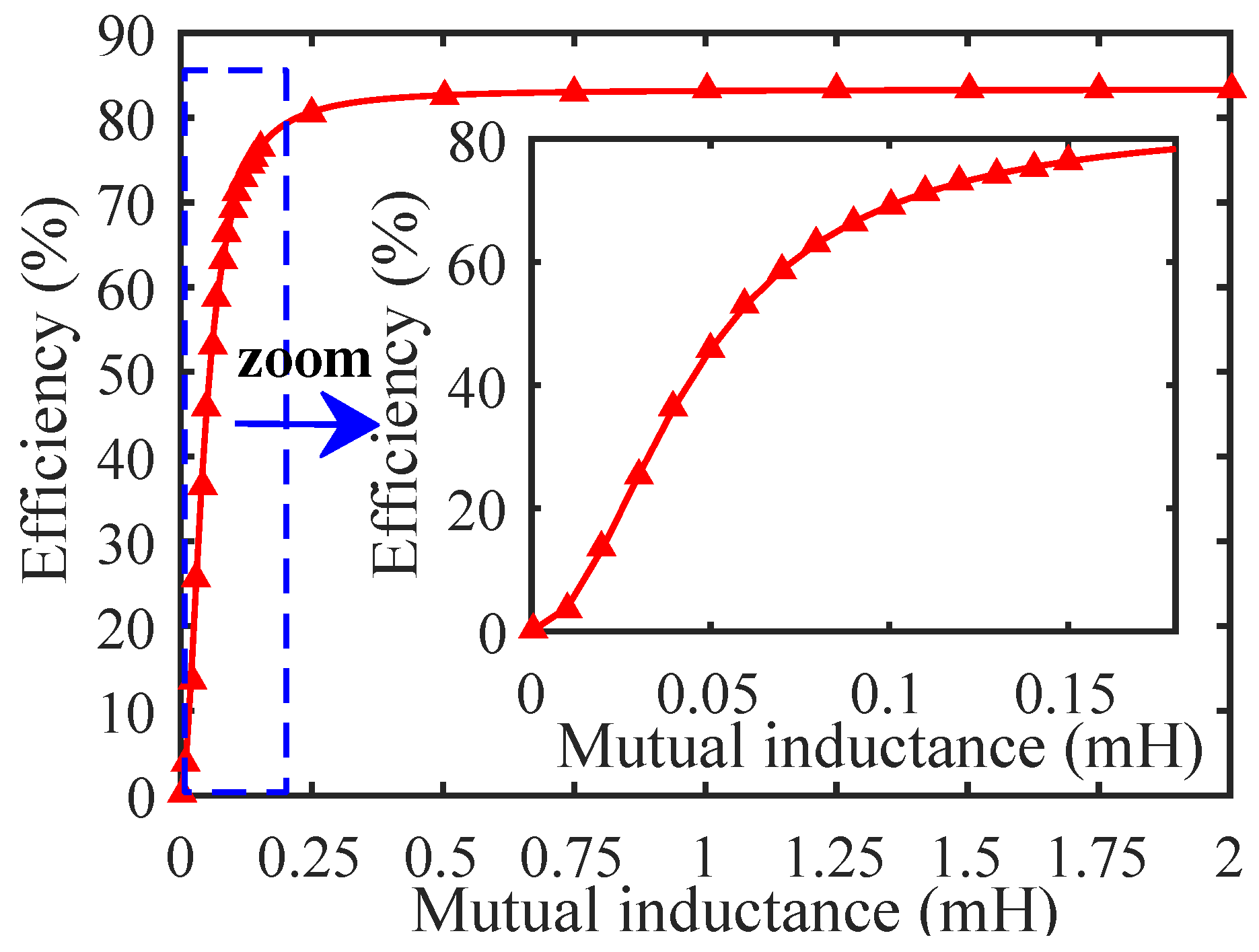
2.1. Influence of Mutual Inductance on WPT System Efficiency

Only the series-series (SS) compensation structure is considered here as an example, and the SS compensation network topology model is shown in Figure 1.
Based on the derivation in [5], the input power P I N and output power P O U T can be expressed as
P I N = U I 1 = U 2 R 1 + ω 0 2 M 2 R 2 + R L
P O U T = I 2 2 R L = ω 0 2 M 2 U 2 R L 2 R 1 + ω 0 2 M 2 R 2 + R L 2 R 2 + R L 2
where ω 0 = 1 C 2 L 2 = 1 C 1 L 1 is the resonant frequency of the system, which is the resonant frequency of the system, and it is generated by the resonance between the compensation capacitor and the self-inductance coil. Near the resonant frequency, the system is approximately resistive, so the effect of reactive power is ignored, and the operating efficiency of the system can be obtained from (1) and (2).
η = ω 0 2 M 2 R L 2 R 1 + ω 0 2 M 2 R 2 + R L R 2 + R L 2
where η is the transmission efficiency of WPT system, R 1 and R 2 are the equivalent resistance of primary and secondary side, and U is the input voltage.
According to the actual parameters in the WPT circuit, let R L = 10 Ω , R 1 = 2 Ω , R 2 = 1.5 Ω , the relationship between mutual inductance and WPT efficiency can be drawn, as shown in Figure 2.
It is obvious that the transmission efficiency increases with the increase of mutual inductance when R L , R 1 , and R 2 are constant. Changing the coil structure may bring a slight change of coil self-induction, but according to Formulas (2) and (3), the transmission power and efficiency of the system are mainly affected by the mutual inductance between the primary side and the secondary side. Therefore, the transmission efficiency of the WPT system can be improved if the mutual inductance of the magnetic coupling structure can be enhanced by changing the shape of the core without changing the coil structure.

2.2. Mutual Inductance Calculation for Central Bulge Ferrite Core

The existing methods for mutual inductance calculation are mostly based on a single pair of coils or coils with a planar core. Therefore, we improved the eigenfunction expansion method proposed in [25,26] to calculate mutual inductance for planar core. Then, the mutual inductance for central bulge ferrite core is calculated based on the improved method.

2.2.1. Mutual Inductance Calculation of Planar Core

The schematic diagram and structure parameters of the planar core, with the transverse profile shown in Figure 3. The radius of the planar core ( R m ), the total thickness of magnetic structure (H), the inner and outer radius of circular coil (R and r), the thickness of the coil (h), and the distance between two coils are described as a 1 , b 3 b 1 , a 2 , a 1 , b 2 b 1 , and 2 b 1 , respectively. Area 1 and Area 5 are the air regions above and below the magnetic coupling structure; Area 2 and Area 4 are the magnetic core region including the magnetic core; Area 3 is the active region including the coil; and Area 5 is axisymmetric about the R axis.
It is assumed that the coil is evenly wound by insulated wires so that the current density J can be regarded as a constant on the whole cross section. The vector potential A in different regions is split into A 1 ( z > b 3 ) , A 2 ( b 2 z b 3 ) , A 3 ( b 2 z b 2 ) , A 4 ( b 3 z b 2 ) , and A 5 ( z b 3 ) . In addition, A 2 is further divided into A 2 ( 1 ) ( b 2 z b 3 , 0 r a 1 ) and A 2 ( 2 ) ( b 2 z b 3 , a 1 r a ) ( A 4 has the same division method). Then, the Laplace and Poisson equations of the vector potential A in the corresponding regions can be obtained as follows,
Δ A 1 , 2 , 4 , 5 = 0 Δ A 3 = μ 0 J ( r , z )
where
J ( r , z ) = J , a 2 r a 1 , b 1 z b 2 0 , otherwise
also, the Laplacian can be written as
Δ = 2 r 2 + 1 r r 1 r 2 + 2 z 2
Moreover, the boundary conditions (A1)–(A11) are listed in the Appendix A.
In the following, this paper employs the matrix symbol to make the subsequent representation clear, and the superscript ( T ) will represent the transposed form of the matrix. Then, we define the eigenvalues p i of the diagonal matrix P are composed of the positive roots of J 1 ( p a ) = 0 , and the eigenvalues q i of the diagonal matrix Q are composed of the positive roots of the eigenvalue equation.
μ r J 1 ( q a 1 ) R 0 ( q a 1 ) = J 0 ( q a 1 ) R 1 ( q a 1 )
R 0 ( q r ) = J 0 ( q r ) Y 1 ( q a ) J 1 ( q a ) Y 0 ( q r ) R 1 ( q r ) = J 1 ( q r ) Y 1 ( q a ) J 0 ( q a ) Y 0 ( q r )
where J n ( x ) and Y n ( x ) are the Bessel functions of the first and second kind, respectively.
Define the elements of the column vector J 1 ( r ) as J 1 ( p i r ) , and the elements of column vectors F ( r ) , G ( r ) are as follows
F ( q i r ) = R 1 ( q i a 1 ) J 1 ( q i r ) G ( q i r ) = J 1 ( q i a 1 ) R 1 ( q i r )
For the primary core, the source function K 1 ( d ) ( z ) can be obtained by the expansion of the eigenfunction μ 0 J ( r ) = J 1 T ( r ) P K 1 ( d ) of region 3 as
K 1 ( d ) ( z ) = K 1 ( d ) , b 1 z b 2 cosh ( z b 1 ) P K 1 ( d ) , z b 1
Similarly, for the secondary core, we have
K 2 ( d ) ( z ) = cosh ( z + b 1 ) P K 2 ( d ) , z b 2 K 2 ( d ) , b 2 z b 1
K ( d ) ( z ) = K 1 ( d ) ( z ) + K 2 ( d ) ( z ) = K 1 ( d ) + cosh ( z + b 1 ) P K 2 ( d ) , b 1 z b 2 cosh ( z b 1 ) P K 1 ( d ) + cosh ( z + b 1 ) P K 2 ( d ) , b 1 z b 1 cosh ( z b 1 ) P K 1 ( d ) + K 2 ( d ) , b 2 z b 1
where the column vectors K 1 ( d ) and K 2 ( d ) have the same elements:
K i = μ 0 J a 2 f 1 ( p n , a 1 ) f 1 ( p n , a 2 ) J 0 2 ( p n a )
f 1 ( p , r ) = π r 2 p J 1 ( p r ) H 0 ( p r ) J 0 ( p r ) H 1 ( p r )
moreover, H n ( x ) is the Struve function.
According to the method of separation of variables, the ansatzes of the vector potential A of the relevant region can be obtained.
A 1 ( r , z ) = J 1 T ( r ) P 1 e ( z b 3 ) P C 1
A 2 ( r , z ) = F T ( r ) G T ( r ) 0 r a 1 a 1 r a · Q 1 e z b 2 Q C 2 + e z b 2 Q D 2 ,
A 3 ( r , z ) = J 1 T ( r ) P 1 [ e ( z + b 2 ) P C 3 + e ( z + b 2 ) P D 3 + K ( d ) ( z ) ]
A 4 ( r , z ) = F T ( r ) G T ( r ) 0 r a 1 a 1 r a · Q 1 e z + b 3 Q C 4 + e z + b 3 Q D 4
A 5 ( r , z ) = J 1 T ( r ) P 1 e ( z + b 3 ) P D 5
In the following calculation, define
S = 0 a r J 1 ( r ) J 1 T ( r ) d r
T = 0 a 1 r J 1 ( r ) F T ( r ) d r + a 1 a r J 1 ( r ) G T ( r ) d r
N = 1 μ r 0 a 1 r F ( r ) F T ( r ) + a 1 a r G ( r ) G T ( r )
Let
V 1 = ( T T ) 1 N , V 2 = P S 1 T Q 1 E 1 ± = V 2 ± V 1 , E 2 ± = V 2 1 ± V 1 1
Substituting the Formulas (15)–(20) into Formulas (A1)–(A11), the following formulas can be obtained:
K 11 K 12 K 21 K 22 C 3 D 3 = W 1 W 2
where
K 11 = ( E 1 e ( b 3 b 2 ) Q E 2 + + E 1 + e ( b 3 b 2 ) Q E 2 ) e 2 b 2 P , K 12 = ( E 1 e ( b 3 b 2 ) Q E 2 + E 1 + e ( b 3 b 2 ) Q E 2 + ) e 2 b 2 P , K 21 = E 1 + e ( b 3 b 2 ) Q E 2 + E 1 e ( b 3 b 2 ) Q E 2 , K 22 = E 1 + e ( b 3 b 2 ) Q E 2 E 1 e ( b 3 b 2 ) Q E 2 + , W 1 = ( E 1 e ( b 3 b 2 ) Q E 2 + + E 1 + e ( b 3 b 2 ) Q E 2 ) K ( d ) ( b 2 ) , W 2 = ( E 1 e ( b 3 b 2 ) Q E 2 + E 1 + e ( b 3 b 2 ) Q E 2 ) K ( d ) ( b 2 )
Solving Equation (24) yields C 3 and D 3 , and then other pending coefficients can be found by Equation (26):
C 2 = 1 2 E 2 + e 2 b 2 P C 3 + E 2 e 2 b 2 P D 3 + E 2 + K ( d ) ( b 2 ) D 2 = 1 2 E 2 e 2 b 2 P C 3 + E 2 + e 2 b 2 P D 3 + E 2 K ( d ) ( b 2 ) C 4 = 1 2 e ( b 3 b 2 ) Q E 2 + C 3 + E 2 D 3 + E 2 K ( d ) ( b 2 ) D 4 = 1 2 e ( b 3 b 2 ) Q E 2 C 3 + E 2 + D 3 + E 2 + K ( d ) ( b 2 ) D 5 = V 2 ( C 4 + D 4 )
When calculating the mutual inductance, the contributions of coils 1 and 2 should be calculated separately. Let K 2 ( d ) = 0 , the contribution of the coil 1 can be directly obtained and distinguished by the superscript “ ( 1 ) ”. Similarly, let K 1 ( d ) = 0 , the contribution of the coil 2 can be obtained, which is represented by the superscript “ ( 2 ) ”. The notation ω is used to indicate the number of turns of the coil, then the analytic expression of mutual inductance can be obtained as follows:
M ( d ) = 1 I 1 I 2 V A 3 ( 1 ) · J ( 2 ) d V = 2 π ω 2 ( a 1 a 2 ) 2 ( b 2 b 1 ) 2 Λ T P 1 2 [ ( e ( b 1 + b 2 ) P e 2 b 2 P ) · C 3 ( 2 ) + ( e 2 b 2 P e ( b 1 + b 2 ) P ) D 3 ( 2 ) + b 1 b 2 K 2 ( d ) ( z ) d z ]
where Λ T = f 1 ( p n , a 1 ) f 2 ( p n , a 2 ) = a 1 a 2 r J 1 T ( r ) d r .

2.2.2. Mutual Inductance Calculation of the Central Bulge Ferrite Core

The schematic diagram and structure parameters of the central bulge ferrite core, with the transverse profile shown in Figure 4.
Similar to the planar core, the transverse profile of central bulge ferrite core is symmetrically divided into several different regions along the r-axis, where the regions 1 and 9 are the respective air zones above and below the magnetic coupling structure, and region 5 is the air zone between two cores. For the convenience of analysis, an imaginary region 3 (air zone) is inserted between region 2 and 4. The upper and lower bounds of region 3 are b 3 and b 2 , respectively ( b 3 is infinitely close to b 2 ). The same assumptions is made for region 7 at the negative direction of the z-axis.
The boundary conditions of each region in Figure 4b can be obtained with the same method in (A1)–(A11), which are not listed here considering the conciseness.
The calculation of the vector potential of the relevant region can be obtained on the basis of variable separation method as (A12)–(A20) show, which is listed in the Appendix A.
Similar to the calculation method in Section 2.2.1, regions 4 and 6 are regarded as source term, and the source function K ( z ) is obtained by the eigenfunction expansion μ 0 J ( r ) = F 2 T ( r ) G 2 T ( r ) Q 2 K in regions 4 and 6:
K 1 ( z ) = K , b 1 z b 2 K 2 ( z ) = K , b 2 z b 1
where the following elements compose the column vectors:
K i = μ 0 J ψ ( q i ) q i N i
and
ψ ( q i ) = J 1 ( q i a 2 ) Y 1 ( q i a ) f 1 ( q i , a 1 ) f 1 ( q i , a 2 ) + J 1 ( q i a 2 ) J 1 ( q i a ) f 2 ( q i , a 1 ) f 2 ( q i , a 2 )
N i = 1 2 J 1 2 ( q i a 2 ) a 2 R 0 2 ( q i a ) a 2 2 R 0 2 ( q i a 2 ) + 1 2 μ r a 2 2 R 1 2 ( q i a ) J 0 2 ( q i a 2 ) ( μ r 1 ) J 1 2 ( q i a 2 )
f 1 ( q , r ) has the same definitions to f 1 ( p , r ) , and
f 2 ( q , r ) = π r 2 q Y 1 ( q r ) H 0 ( q r ) Y 0 ( q r ) H 1 ( q r )
F 1 T ( r ) , G 1 T ( r ) , and Q 1 , and F T ( r ) , G T ( r ) , and Q have the same eigenvalue, and the eigenvalues of F 2 T ( r ) , G 2 T ( r ) , Q 2 are given by
μ r J 1 ( q a 2 ) R 0 ( q a 2 ) = J 0 ( q a 2 ) R 1 ( q a 2 )
The undetermined coefficients C 1   C 8 and can be obtained by the method shown in Section 2.2.1, and then we can get the mutual inductance:
M = 1 I 1 I 2 V A 4 ( 2 ) · J ( 1 ) d V = 2 π ω 2 ( a 1 a 2 ) 2 ( b 2 b 1 ) 2 ψ T ( Q 2 ) ( Q 2 1 ) 2 · [ ( 1 e ( b 2 b 1 ) Q ) C 4 ( 2 ) + ( e ( b 2 b 1 ) Q 1 ) D 4 ( 2 ) ]

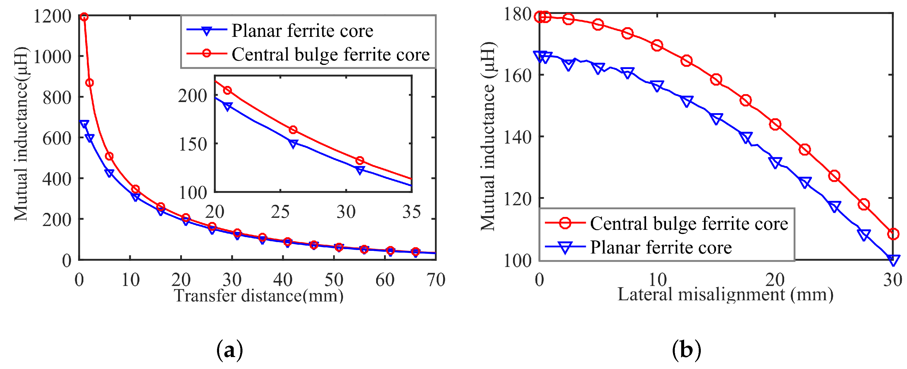
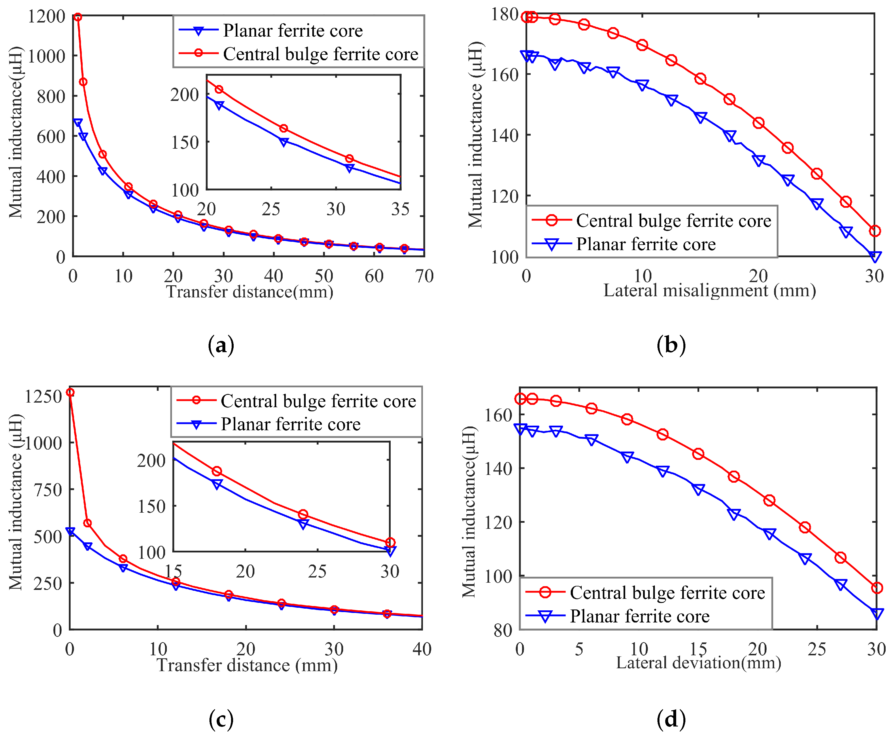
2.2.3. Comparative Analysis

For Equations (27) and (34), owing to the constant changes of parameters in the diagonal matrix P and Q, the direct comparison seems to be impractical. The magnetic permeability of the central bulge in Figure 4b is set to be μ x . Therefore, it is equivalent to the planar magnetic coupling structure shown in Figure 3b, which means when μ x = μ 0 , the results of (34) M is equal to M ( d ) , which is calculated from (27).
Let m = 2 π ω 2 ( a 1 a 2 ) 2 ( b 2 b 1 ) 2 . After extracting the common factor by (33), we can obtain
M = m φ T ( Q x ) Q x 2 ( e ( b 2 b 1 ) Q x 1 ) ( D 4 ( 2 ) C 4 ( 2 ) )
As for D 4 ( 2 ) C 4 ( 2 ) , it is a column vector related to Q x , and we define
E ( Q x ) = D 4 ( 2 ) C 4 ( 2 )
A = Q x 2 ( e ( b 2 b 1 ) Q x 1 )
For the diagonal matrix Q x , there is
m λ min ( A T A ) | φ ( Q x ) | | E ( Q x ) | m φ T ( Q x ) A E ( Q x ) m φ T ( Q x ) A E ( Q x ) m λ max ( A T A ) | φ ( Q x ) | | E ( Q x ) |
λ max ( A T A ) = λ max ( A 2 ) = λ max ( A ) 2 = λ max ( A )
where λ min ( A ) and λ max ( A ) are the minimum and maximum eigenvalues of the matrix A, respectively. When the magnetic permeability μ x of the intermediate bulge changes, the eigenvalues of the positive diagonal array Q x will change accordingly.
μ x J 1 ( q a 2 ) R 0 ( q a 2 ) = J 0 ( q a 2 ) R 1 ( q a 2 )
To seek the solution of (40), let H 1 ( q ) = J 0 ( q a 2 ) R 1 ( q a 2 ) , H 2 ( q ) = μ 0 J 1 ( q a 2 ) R 0 ( q a 2 ) , H 3 ( q ) = μ 3 J 1 ( q a 2 ) R 0 ( q a 2 ) , whose function images are shown in Figure 5. In Figure 5, the purple, black, and green dots represent the common intersection points of three functions, intersection points of H 1 and H 2 , and intersection points of H 1 and H 3 . It is clear that black dots are more dense than green dots, which means that when μ x is increased, most of the values of q i will increase, and only a small fraction will decrease with the same i. As the oscillation of the Bessel function is gradually attenuated, when the value of q i is comparatively large, even if the change of q i causes the diagonal matrix Q x to change, but the fluctuation of | φ ( Q x ) | | E ( Q x ) | is small, so only λ ( A ) is discussed below.
λ ( A ) can be written as λ ( A ) = q 2 ( e ( b 2 b 1 ) q 1 ) , for that Q x is positive definite diagonal matrix. In practical applications, the thickness of the coil is generally about 1–5 mm, so let 1 b 2 b 1 5 . When b = b 2 b 1 changes, the curve of λ ( A ) is shown in Figure 6.
As can be seen from the Figure 6, when q > 2 , λ ( A ) is monotonically increasing. Therefore, for the diagonal matrix Q x , the eigenvalues q i is mostly located in the monotonic increasing zone, and a very small portion is located in the monotonic decreasing zone. Therefore, when the vast majority of q i in the monotonic increasing zone increases, λ ( A ) will increase, and the mutual inductance M will increase. Therefore, when the magnetic permeability of the intermediate bulge is increased, the mutual inductance is increased, which theoretically proves that the mutual inductance of the proposed core is greater than that of the planar core.
In summary, from the perspective of mathematical calculation, the proposed core can enhance the mutual inductance of the magnetic coupling structure by improving the magnetic field coupling relationship, thereby improving the system efficiency.

3. Parameter Design

To enhance the system output capability, the parameters of the magnetic coupling structure need to be optimized to achieve a larger mutual inductance. To verify the theoretical results in the previous section from the experimental view, combined with the actual structural parameters of the planar core, the finite element analysis software Maxwell is used to simulate and optimize the central bulge ferrite core. Moreover, the actual structure parameters of the planar core are shown in Table 1.
According to the design requirements of laboratory prototype, the selection of radio transmission distance d = 24 mm is fixed in the design. In the early design work, the parameter characteristics of different material, the shape of magnetic core, and the ability to resist horizontal migration were comprehensively considered. The volume limit of the prototype was also taken into account. In this design, the final material was PC95 ferrite and the circular magnetic core with a radius of 60 mm. Considering the influence of magnetic core thickness on mutual inductance and coupling coefficient, as well as the factors such as volume limitation and production cost, the final thickness of the magnetic core is selected as 10 mm. Considering the influence of coil wire diameter on self-inductance, mutual inductance, coupling coefficient, rated current, etc., the final coil adopts Leeds wire of 150 strands/turns, and the wire diameter is 1.7 mm. In this study, the layer number, outer diameter, inner diameter, and other parameters of the coil will be carefully optimized, because these parameters will have an important impact on the mutual inductance and coupling coefficient of the system, and then affect the effect of the raised magnetic core proposed in this study to improve the efficiency of the wireless power supply device. Taking into account the volume constraint of the prototype, the optimization range of the coil layer is 1–3 layers, the optimization range of the outer diameter is 0–60 mm, and the optimization range of the inner diameter is 0–40 mm. Next, we will choose a simple and practical optimization method to realize the design of the parameters such as the number of layers, outside diameter and inside diameter of the coil.
First, the number of winding layers of the coil is simulated and optimized. In the case where the coil is wound around 1 layer, 2 layers, and 3 layers, the mutual inductance of the magnetic coupling structure is simulated and analyzed, respectively, and the results are shown in Table 2 (in this paper’s simulation and physical verification, 150 shares of Litz copper wire are used, and the wire diameter is 1.7 mm).
It can be seen from Table 1 that when the coil is wound only around one layer, the height of the intermediate is small, and the internal resistance of primary and secondary coils is small, but mutual inductance is significantly lower than that of the multi-layer coil, so that the transmission capacity and efficiency of the whole system are low. When the coil is wound around the three layers, although the mutual inductance is higher than that of the two-layer coil, the internal resistance of the two coils will increase sharply, which is still not conducive for the efficiency improvement. Thus, when the coil is wound around two layers, the transmission capacity and efficiency of the system are better.
Select two layers ( h = 3.4 mm ) as the optimized parameters, and under this condition, the changes of mutual inductance with R and r are shown in Figure 7.
It is obvious from Figure 7 that the mutual inductance M increases steadily with the increase of the outer diameter R; when R is small, M decreases with the increase of the inner diameter r. When R is larger, the M increases at first and then decreases with the increase of r. Therefore, to obtain a higher M, the maximum outer diameter R = 60 mm is chosen. Under this circumstance, when 0 < r < 12 mm, M increases as r increases; when r = 12 mm, the maximum value is 183.3944 uH, when r > 12 mm, M decreases as r increases. In summary, according to the finite element simulation results and actual situation, the optimized parameters are shown in Table 3.

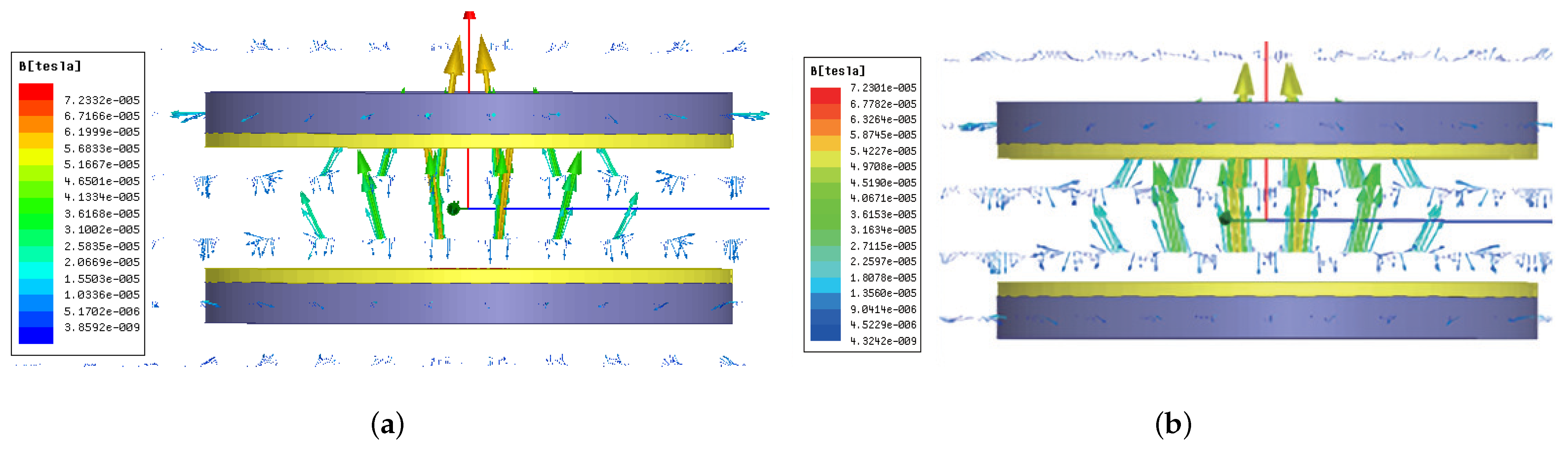
4. Simulation Comparison

To verify the effectiveness of the proposed core in enhancing the mutual inductance, 3D models of the proposed core and the planar core are built in Maxwell. In the simulation and experimental verification, we set the core material as PC95 ferrite. Leeds lines with a diameter of 1.7mm and 150 strands/turns were used. The selected parameters of the proposed core are shown in Table 3. Moreover, to make the comparison result convincing, the structural parameters of the planar core used in this paper are listed in Table 4.
Figure 8 and Figure 9 show the distribution of magnetic field and magnetic lines of force under the same conditions for two magnetic coupling structures.
It can be seen from Figure 8 and Figure 9 that the magnetic coupling structure using the proposed core has greater magnetic field intensity than that using planar core and the magnetic line of force is denser. It is clear from the comparison that due to the effective utilization of the remaining space, the proposed core can effectively enhance the magnetic field between the primary and secondary side. The magnetic leakage is reduced, thereby the mutual inductance can be enhanced and the goal of improving system transmission efficiency can be achieved.
The conditions of mutual inductance M when transmission distance and the lateral misalignment change are simulated through the finite element simulation model of the two magnetic coupling structures and the results are shown in Figure 10.
As shown in Figure 10, the curve indicated by the dot indicates the mutual inductance of the magnetic coupling structure with the proposed core, and the curve indicated by the triangle indicates the mutual inductance of the magnetic coupling structure with the planar core. As shown in Figure 10a, as the transmission distance increases, the mutual inductance of the two magnetic coupling structures decreases, but the mutual inductance of the magnetic coupling structure with the proposed core is always greater than that of the magnetic coupling structure with the planar core. Moreover, this advantage is more obvious in the case of short distance transmission. As shown in Figure 10b, as the lateral misalignment increases, the mutual inductance of the two magnetic coupling structures decreases, but the mutual inductance of the magnetic coupling structure is always greater than that of magnetic coupling structure with planar core, which means that the proposed core has the better anti-misalignment capability.

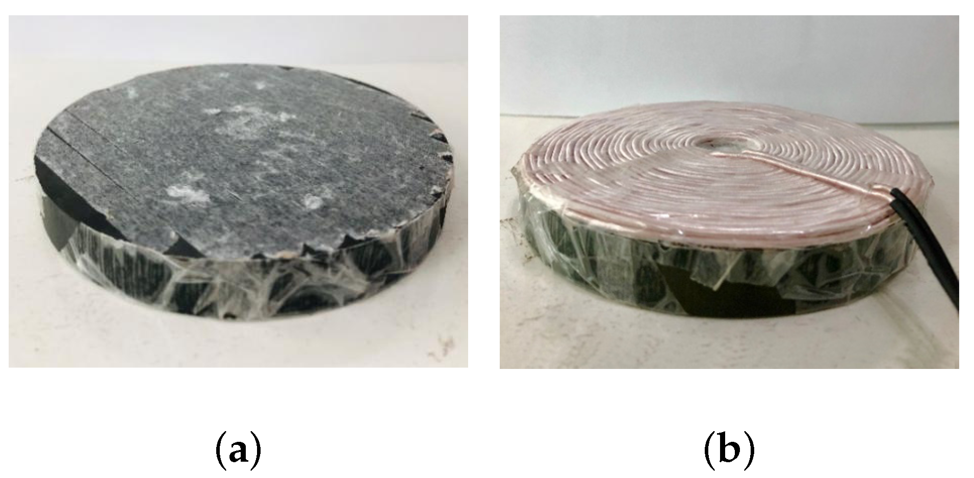
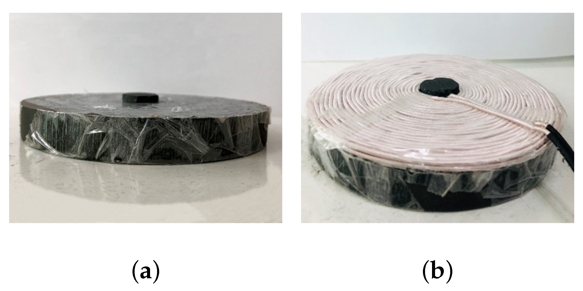
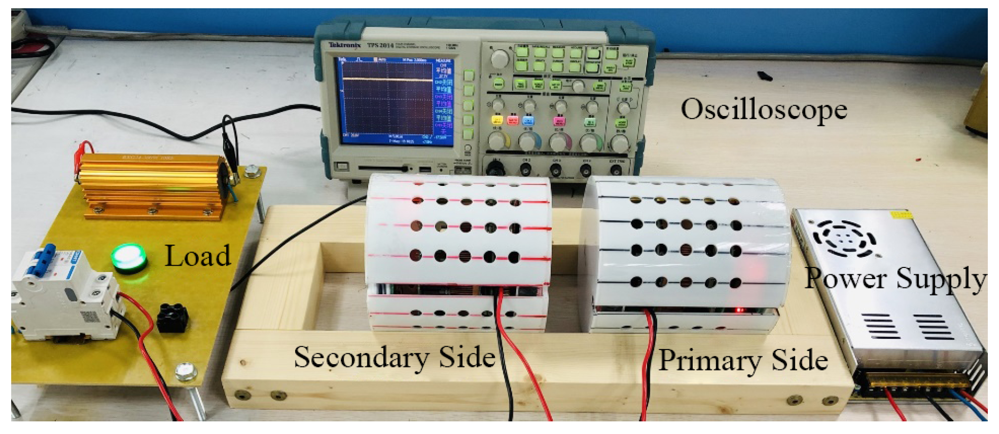
5. Experimental Verification

To verify the theory and simulation results obtained in Section 3 and Section 4, the physical models of the planar and proposed core are made as shown in Figure 11 and Figure 12.
First, the mutual inductance’s curves with transmission distance and lateral misalignment are measured when magnetic coupling structures are not connected to the whole system, and the results are indicated in Figure 13.
It can be seen from Figure 13 that for the single magnetic coupling structure, the proposed core can greatly improve the mutual inductance of the magnetic coupling structure, which also verifies the results of the theoretical analysis and simulation. Furthermore, Figure 13 compares the curves of mutual inductance with wireless power transmission distance and lateral migration of the two magnetic coupling structures measured experimentally and obtained using FSM. As can be seen from the figure, there is only a slight difference between the curves measured by the experiment and the curves obtained by the simulation, which is mainly caused by the complexity of the experimental environment and the device and the imperfection of the simulation. However, the experimental curve and simulation curve are basically the same in terms of variation trend and variation range, which fully proves the correctness and validity of the above theory and simulation analysis.
Then, the two magnetic coupling structures are, respectively, connected to the WPT system for experimental verification of the transmission efficiency.The prototype of the wireless power transfer device is shown in Figure 14. The power supply provides a 28 V DC voltage.
After accessing the power transmitting terminal, energy is wirelessly transmitted to the power receiving terminal and then connected to the load. Wherein, the power transmitting and receiving terminal is fixed on the bracket capable of adjusting the transmission distance.
Figure 15 shows the curves of transmission efficiency at several different load levels when the two types of magnetically coupled structures are accessed to a WPT system, respectively.
It can be seen from Figure 15 that, compared with the WPT system with planar core, the efficiency of the WPT system with the proposed core is significantly improved in terms of effective transmission distance, and their variation trend with the distance curve is the same. Furthermore, the transmission efficiency of the WPT system with the proposed core shows a considerable advantage over long distances. When the load is 19.5 Ω , the maximum transmission efficiency of the system can be increased to 73.5 % and the maximum efficiency improvement rate is 23.3 % , the experimental results are basically in line with the preliminary expectations of theoretical analysis and simulation.
However, we also noticed that when the load resistance is large, the transmission efficiency decreases with the decrease of the distance before the maximum efficiency is achieved, and even the transmission efficiency of the proposed core becomes lower than that of the planar core. This is not consistent with the results of theoretical analysis and simulation. For this question, we make the following explanation:
(1)
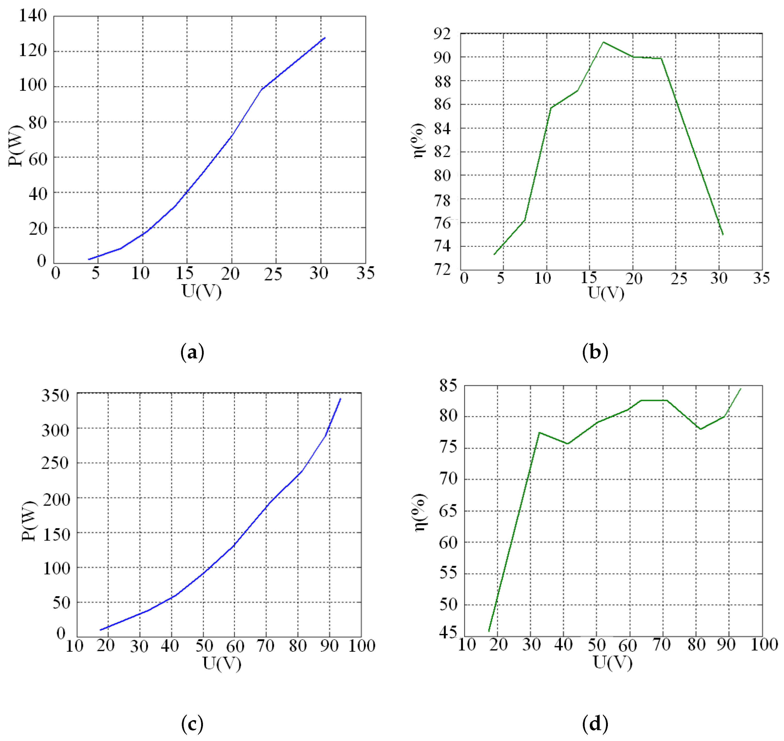
The theoretical analysis does not consider the case where the impedance mismatch causes the input impedance to increase. In case of short-distance transmission, the WPT system works in the over-coupled region and there is frequency splitting.
(2)
The self-inductance and mutual inductance of the magnetic coupling structure are increased with the proposed core, but the compensation capacitance of the system does not change, which leads to system mismatch, resulting in the first half of the efficiency drop, and the best matching point is shifted.
(3)
The theoretical analysis and simulation does not include the core loss of the core. Due to the increase in the volume of the core portion, the magnetic loss of the magnetic coupling system may increase, resulting in a decrease of efficiency in the first half.
Figure 15 shows the curves of transmission efficiency during lateral misalignment in a WPT system with two types of cores at the load of and transmission distance of 30 mm.
It can be seen from Figure 16 that when the lateral offset is small, there is almost no difference between the transmission efficiency of the WPT system with two cores, but the WPT system with the proposed core exhibits a huge advantage in anti-misalignment. Moreover, this is consistent with the results of theoretical analysis and simulation.
The curves at 50 Ω and 10.5 Ω are shown in Figure 17, respectively. When the load is 50 Ω , the output power increases with the supply voltage; the system efficiency first increases, and then decreases with the increase of the power supply voltage. When the input voltage is 16.6 V, the system efficiency can reach 91.27% and reach the peak. When the load is 10.5 Ω , the output power also increases with the increase of the supply voltage. When the input voltage is 93.6 V, the output power can reach 342.6 W; the reason why the efficiency peak does not appear here is that the peak point of efficiency has not been reached. When the power supply voltage is increased, it will appear. However, due to the aging of the proportional transformer in the experiment and the serious ignition, for the sake of the safety of the experiment, the pressure experiment is no longer carried out.
Except for the load of 10.5 Ω and the power supply voltage of 17.3 V, the system efficiency does not reach 70%, and the system efficiency reaches 70% under other loads and power supply voltages.

6. Conclusions

In this paper, a novel structure of the central bulge ferrite core is proposed, which can effectively increase the mutual inductance of the magnetic coupling without increasing the size of the WPT system, thereby significantly improving the power transmission efficiency. The improved mathematical models to calculate the mutual inductance of the planar core and the proposed central bulge core are established, and the Fourier–Bessel transform is used to analyze the boundary conditions of the magnetic field. It is concluded that the mutual inductance of the proposed central bulge core is greater than that of the planar core theoretically. In addition, this paper uses the finite element simulation software Maxwell to optimize the proposed core’s structure parameters to achieve better performance. Finally, a prototype test is set up for experimental verification. The experiment proves that the central bulge ferrite core is superior to the planar core in terms of power transmission distance and has higher tolerance in misalignment. The case study shows that when the system load is 19.5 Ω , the maximum power transmission efficiency of the system can be increased to 73.5 % , with a maximum efficiency improvement rate of 23.3 % .

Author Contributions

Conceptualization, H.X., R.H. and H.S.; methodology, H.X., R.H. and H.S.; software, H.X. and R.H.; validation, H.X. and R.H.; formal analysis, H.X. and R.H.; investigation, H.X. and R.H.; resources, H.X., R.H. and H.S.; data curation, H.X. and R.H.; writing—original draft preparation, H.X. and R.H.; writing—review and editing, H.X. and R.H.; visualization, H.X. and R.H.; supervision, H.X., R.H. and H.S.; project administration, H.S.; funding acquisition, H.S. All authors have read and agreed to the published version of the manuscript.

Funding

This work is supported by the National Natural Science Foundation of China (No. 61773137), the Natural Science Foundation of Shandong Province (Nos. ZR2019MF030 and ZR2018PEE018), China Postdoctoral Science Foundation (No. 2018M641830).

Institutional Review Board Statement

Not applicable.

Informed Consent Statement

Not applicable.

Data Availability Statement

Not applicable.

Acknowledgments

Not applicable.

Conflicts of Interest

The authors declare no conflict of interest.

Appendix A

Formulas (A1)–(A11) are the boundary conditions of the model mentioned in Section 2.2.1.
A 1 , 2 , 3 , 4 , 5 ( a , z ) = 0
A 2 ( 1 ) ( a 1 , z ) = A 2 ( 2 ) ( a 1 , z )
1 μ r ( r ) A 2 ( 1 ) r r = a 1 = ( r ) A 2 ( 2 ) r r = a 1
A 1 ( r , b 3 ) = A 2 ( r , b 3 )
A 1 z z = b 3 = 1 μ r A 2 z z = b 3 , 0 r a 1 A 2 z z = b 3 , a 1 r a
A 2 ( r , b 2 ) = A 3 ( r , b 2 )
A 3 z z = b 2 = 1 μ r A 2 z z = b 2 , 0 r a 1 A 2 z z = b 2 , a 1 r a
A 3 ( r , b 2 ) = A 4 ( r , b 2 )
A 3 z z = b 2 = 1 μ r A 4 z z = b 2 , 0 r a 1 A 4 z z = b 2 , a 1 r a
A 4 ( r , b 3 ) = A 5 ( r , b 3 )
A 5 z z = b 3 = 1 μ r A 4 z z = b 3 , 0 r a 1 A 4 z z = b 3 , a 1 r a
Formulas (A12)–(A20) represent an analytical expression of magnetic vector A in the relevant region based on the method of separating variables
A 1 ( r , z ) = J 1 T ( r ) P 1 e ( z b 4 ) P C 1
A 2 ( r , z ) = F 1 T ( r ) G 1 T ( r ) 0 r a 1 a 1 r a · Q 1 1 e z b 3 Q 1 C 2 + e z b 3 Q 1 D 2
A 3 ( r , z ) = J 1 T ( r ) P 1 [ e ( z b 2 ) P C 3 + e ( z b 2 ) P D 3 ]
A 4 ( r , z ) = F 2 T ( r ) G 2 T ( r ) 0 r a 2 a 2 r a · Q 2 1 e z b 1 Q 2 C 4 + e z b 1 Q 2 D 4 + K ( z )
A 5 ( r , z ) = J 1 T ( r ) P 1 [ e ( z + b 1 ) P C 5 + e ( z + b 1 ) P D 5 ]
A 6 ( r , z ) = F 2 T ( r ) G 2 T ( r ) 0 r a 2 a 2 r a · Q 2 1 e z + b 2 Q 2 C 6 + e z + b 2 Q 2 D 6 + K ( z )
A 7 ( r , z ) = J 1 T ( r ) P 1 [ e ( z + b 3 ) P C 7 + e ( z + b 2 ) P D 7 ]
A 8 ( r , z ) = F 1 T ( r ) G 1 T ( r ) 0 r a 1 a 1 r a · Q 1 1 e z + b 4 Q 1 C 8 + e z + b 4 Q 1 D 8
A 9 ( r , z ) = J 1 T ( r ) P 1 e ( z + b 4 ) P D 9

References

  1. Jiang, Y.; Wang, L.; Wang, Y. Analysis, Design and Implementation of Accurate ZVS Angle Control for EV Battery Charging in Wireless High Power Transfer. IEEE Trans. Ind. Electron. 2019, 60, 4075–4085. [Google Scholar] [CrossRef]
  2. Choi, S.Y.; Gu, B.W.; Jeong, S.Y. Modern Advances in Wireless Power Transfer Systems for Roadway Powered Electric Vehicles. IEEE Trans. Ind. Electron. 2016, 63, 6533–6545. [Google Scholar]
  3. Liu, C.; Jiang, C.; Song, J.; Chau, K.T. An Effective Sandwiched Wireless Power Transfer System for Charging Implantable Cardiac Pacemaker. IEEE Trans. Ind. Electron. 2019, 66, 4108–4117. [Google Scholar] [CrossRef]
  4. Olatinwo, S.O.; Joubert, T.H. Energy Efficient Solutions in Wireless Sensor Systems for Water Quality Monitoring: A Review. IEEE Sens. J. 2019, 19, 1596–1625. [Google Scholar] [CrossRef]
  5. Zhou, J.; Zhang, B.; Xiao, W.; Qiu, D. Nonlinear Parity-Time-Symmetric Model for Constant Efficiency Wireless Power Transfer: Application to a Drone-in-Flight Wireless Charging Platform. IEEE Trans. Ind. Electron. 2019, 66, 4097–4107. [Google Scholar] [CrossRef]
  6. Basar, M.R.; Ahmad, M.Y.; Cho, J. Stable and High-Efficiency Wireless Power Transfer System for Robotic Capsule Using a Modified Helmholtz Coil. IEEE Trans. Ind. Electron. 2017, 64, 1113–1122. [Google Scholar] [CrossRef]
  7. Hui, S.Y.R.; Zhong, W.; Lee, C.K. A Critical Review of Recent Progress in Mid-Range Wireless Power Transfer. IEEE Trans. Power Electron. 2014, 29, 4500–4511. [Google Scholar] [CrossRef] [Green Version]
  8. Mayordomo, I.; Dräger, T.; Spies, P. An Overview of Technical Challenges and Advances of Inductive Wireless Power Transmission. Proc. IEEE 2013, 101, 1302–1311. [Google Scholar] [CrossRef]
  9. Zhong, W.X.; Zhang, C.; Liu, X.; Hui, S.Y.R. A methodology for making a three-coil wireless power transfer system more energy efficient than a two-coil counterpart for extended transfer distance. IEEE Trans. Power Electron. 2016, 30, 933–942. [Google Scholar] [CrossRef]
  10. Ye, Z.H.; Sun, Y.; Dai, X.; Tang, C.S. Energy Efficiency Analysis of U-coil Wireless Power Transfer System. IEEE Trans. Power Electron. 2016, 31, 4809–4817. [Google Scholar] [CrossRef]
  11. Zhang, Z.; Pang, H.; Georgiadis, A. Wireless Power Transfer—An Overview. IEEE Trans. Ind. Electron. 2019, 66, 1044–1058. [Google Scholar] [CrossRef]
  12. Raju, S.; Wu, R.; Chan, M.; Yue, C.P. Modeling of Mutual Coupling Between Planar Inductors in Wireless Power Applications. IEEE Trans. Power Electron. 2014, 29, 481–490. [Google Scholar] [CrossRef]
  13. Waters, B.H.; Mahoney, B.J.; Lee, G. Optimal coil size ratios for wireless power transfer applications. In Proceedings of the 2014 IEEE International Symposium on Circuits and Systems (ISCAS), Melbourne, Australia, 1–5 June 2014; pp. 2045–2048. [Google Scholar]
  14. Cove, S.R.; Ordonez, M.; Shafiei, N. Improving Wireless Power Transfer Efficiency Using Hollow Windings with Track-Width-Ratio. IEEE Trans. Power Electron. 2016, 31, 6524–6533. [Google Scholar] [CrossRef]
  15. Jeong, S.Y.; Kwak, H.G.; Jang, G.C. Dual-Purpose Nonoverlapping Coil Sets as Metal Object and Vehicle Position Detections for Wireless Stationary EV Chargers. IEEE Trans. Power Electron. 2018, 33, 7387–7397. [Google Scholar] [CrossRef]
  16. Moon, S.C.; Moon, G.W. Wireless Power Transfer System with an Asymmetric 4-Coil Resonator for Electric Vehicle Battery Chargers. In Proceedings of the 2015 IEEE Applied Power Electronics Conference and Exposition (APEC), Charlotte, NC, USA, 15–19 March 2015; Volume 31, pp. 6844–6854. [Google Scholar]
  17. Lee, C.K.; Zhong, W.X.; Hui, S.Y.R. Effects of Magnetic Coupling of Nonadjacent Resonators on Wireless Power Domino-Resonator Systems. IEEE Trans. Power Electron. 2012, 27, 1905–1916. [Google Scholar] [CrossRef] [Green Version]
  18. Chen, L.; Liu, S.; Zhou, Y.C.; Cui, T.J. An Optimizable Circuit Structure for High-Efficiency Wireless Power Transfer. IEEE Trans. Ind. Electron. 2013, 60, 339–349. [Google Scholar] [CrossRef]
  19. Yeo, T.D.; Kwon, D.S.; Khang, S.T. Design of Maximum Efficiency Tracking Control Scheme for Closed Loop Wireless Power Charging System Employing Series Resonant Tank. IEEE Trans. Power Electron. 2017, 32, 471–478. [Google Scholar] [CrossRef]
  20. Kim, H.; Song, C.; Kim, D.H.; Jung, D.H. Coil Design and Measurements of Automotive Magnetic Resonant Wireless Charging System for High-Efficiency and Low Magnetic Field Leakage. IEEE Trans. Microw. Theory Tech. 2016, 64, 383–400. [Google Scholar] [CrossRef]
  21. Li, Z.; Zhu, C.; Jiang, J.; Song, K. A 3 kW Wireless Power Transfer System for Sightseeing Car Supercapacitor Charge. IEEE Trans. Power Electron. 2017, 32, 3301–3316. [Google Scholar] [CrossRef]
  22. Budhia, M.; Covic, G.A.; Boys, J.T. Design and Optimization of Circular Magnetic Structures for Lumped Inductive Power Transfer Systems. IEEE Trans. Power Electron. 2011, 26, 3096–3108. [Google Scholar] [CrossRef]
  23. Mohammad, M.; Choi, S.; Islam, Z. Core Design and Optimization for Better Misalignment Tolerance and Higher Range Wireless Charging of PHEV. IEEE Trans. Transp. Electrif. 2017, 3, 445–453. [Google Scholar] [CrossRef]
  24. Wang, M.; Feng, J.; Shi, Y.; Shen, M. Demagnetization Weakening and Magnetic Field Concentration With Ferrite Core Characterization for Efficient Wireless Power Transfer. IEEE Trans. Ind. Electron. 2019, 66, 1842–1851. [Google Scholar] [CrossRef]
  25. Luo, Y. Field and inductance calculations for coaxial circular coils with magnetic cores of finite length and constant permeability. IET Electr. Power Appl. 2017, 11, 1254–1264. [Google Scholar] [CrossRef]
  26. Lubin, T.; Berger, K.; Rezzoug, A. Inductance and force calculation for axisymmetric coil systems including an iron core of finite length. Prog. Electromagn. Res. 2012, 41, 377–396. [Google Scholar] [CrossRef] [Green Version]
Figure 1. Equivalent circuit topology of WPT system with SS compensation network.
Energies 14 05111 g001
Figure 2. Curve of mutual inductance and efficiency when R L = 10 Ω , R 1 = 2 Ω , R 2 = 1.5 Ω .
Energies 14 05111 g002
Figure 3. Planar core: (a) Schematic diagram and structure parameters; (b) Transverse profile.
Energies 14 05111 g003
Figure 4. Central bulge ferrite core: (a) Schematic diagram and structure parameters; (b) Transverse profile.
Energies 14 05111 g004
Figure 5. Changes of the eigenvalues for Q x when μ x change.
Energies 14 05111 g005
Figure 6. Curve of λ ( A ) under different b.
Energies 14 05111 g006
Figure 7. Changes of mutual inductance with R and r.
Energies 14 05111 g007
Figure 8. Comparison of two magnetic coupling structures’ magnetic field distribution: (a) Magnetic field distribution of planar core; (b) Magnetic field distribution of proposed core.
Energies 14 05111 g008
Figure 9. Comparison of two magnetic coupling structures’ magnetic line of force: (a) Magnetic line of force of planar core; (b) Magnetic line of force of the proposed core.
Energies 14 05111 g009
Figure 10. Comparison of two magnetic coupling structures’ magnetic line of force: (a) Curves of M when transmission distance changes; (b) Curves of M when lateral misalignment changes.
Energies 14 05111 g010
Figure 11. Prototype of planar core: (a) Prototype of the single planar core; (b) Prototype of the planar core with coil.
Energies 14 05111 g011
Figure 12. Prototype of the proposed core: (a) Prototype of the single proposed core; (b) Prototype of the proposed core with coil.
Energies 14 05111 g012
Figure 13. Comparison of two magnetic coupling structures’ magnetic line of force: (a) Curves of M when transmission distance changes in simulation; (b) Curves of M when lateral misalignment changes in simulation; (c) Curves of M when transmission distance changes in the experiment; (d) Curves of M when lateral misalignment changes in the experiment.
Energies 14 05111 g013
Figure 14. Prototype of the wireless power transfer device.
Energies 14 05111 g014
Figure 15. Curves of transmission efficiency at different load levels.
Energies 14 05111 g015
Figure 16. Curves of transmission efficiency during lateral misalignment.
Energies 14 05111 g016
Figure 17. Varying supply voltage test system performance: (a) Experimental output power curve of variable power supply voltage—Load 50 Ω ; (b) Experimental system efficiency curve with variable power supply voltage—Load 50 Ω ; (c) Experimental output power curve of variable power supply voltage—Load 10.5 Ω ; (d) Experimental system efficiency curve with variable power supply voltage—Load 10.5 Ω .
Energies 14 05111 g017
Table 1. Actual structure parameters of planar core.
Structure ParametersSize/mm
The total thickness of magnetic coupling structure (H)10
Core radius ( R m )60
Transmission distance (d)24
Coil outer diameter (R)60
Coil inner diameter (r)10
Table 2. Mutual inductance under different coil layer.
Coil Layer L 1 / uH L 2 / uH M / uHk
194.449094.420548.56750.5143
2357.7960357.5945173.14040.4840
3772.4861772.4096353.38360.4575
Table 3. Optimized parameters of the proposed core.
Optimized ParameterSize/mm
The total thickness of magnetic coupling structure (H)10
Core radius ( R m )60
Height of intermediate bulge (h)3.4
Transmission distance (d)24
Coil outer diameter (R)60
Coil inner diameter (r)10
Table 4. Structural parameters of the planar core.
Structure ParameterSize/mm
Total thickness of magnetic coupling structure (H)10
Core radius ( R m )60
Coil thickness (h)3.4
Transmission distance (d)24
Coil outer diameter (R)60
Coil inner diameter (r)10
Publisher’s Note: MDPI stays neutral with regard to jurisdictional claims in published maps and institutional affiliations.

