
Traffic Noise Modelling Using Land Use Regression Model Based on Machine Learning, Statistical Regression and GIS


 ,
,  and
and
Abstract
:1. Introduction
2. Related Work
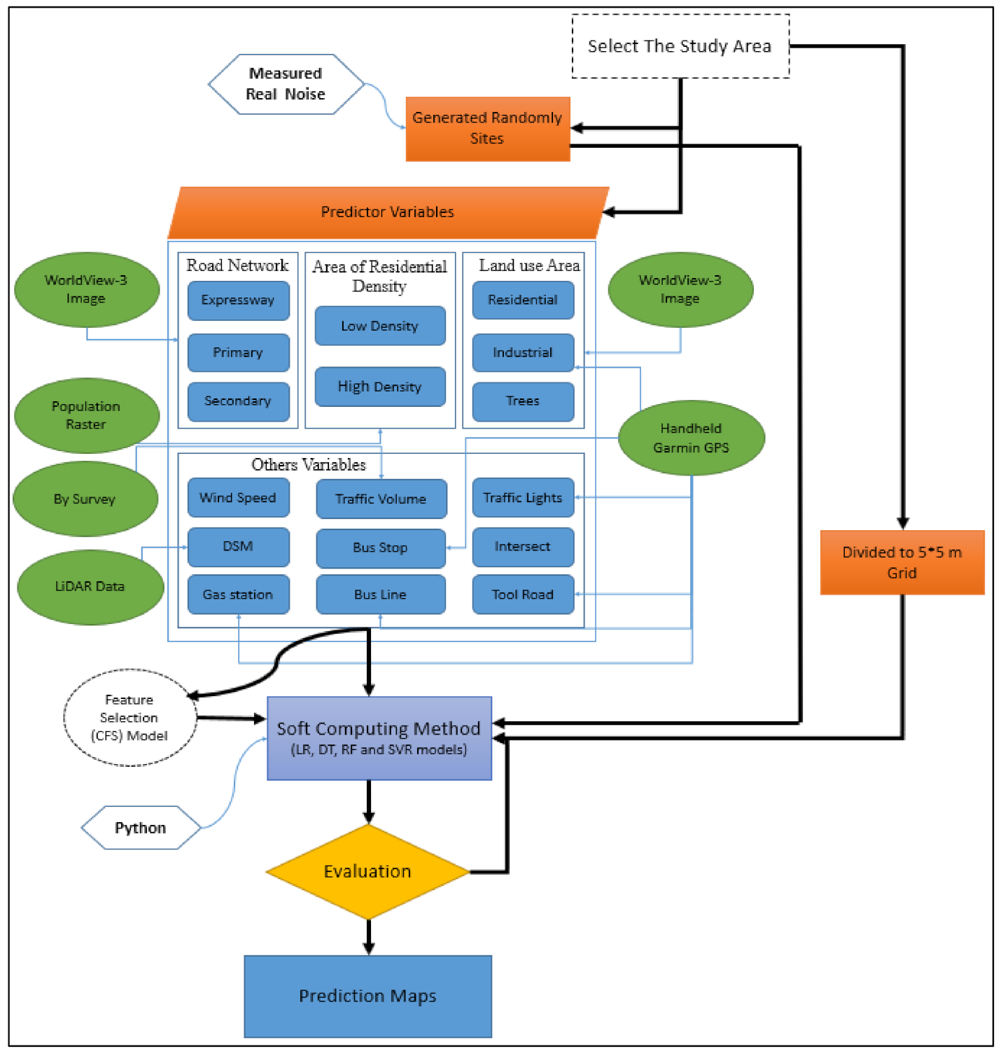
3. Methods
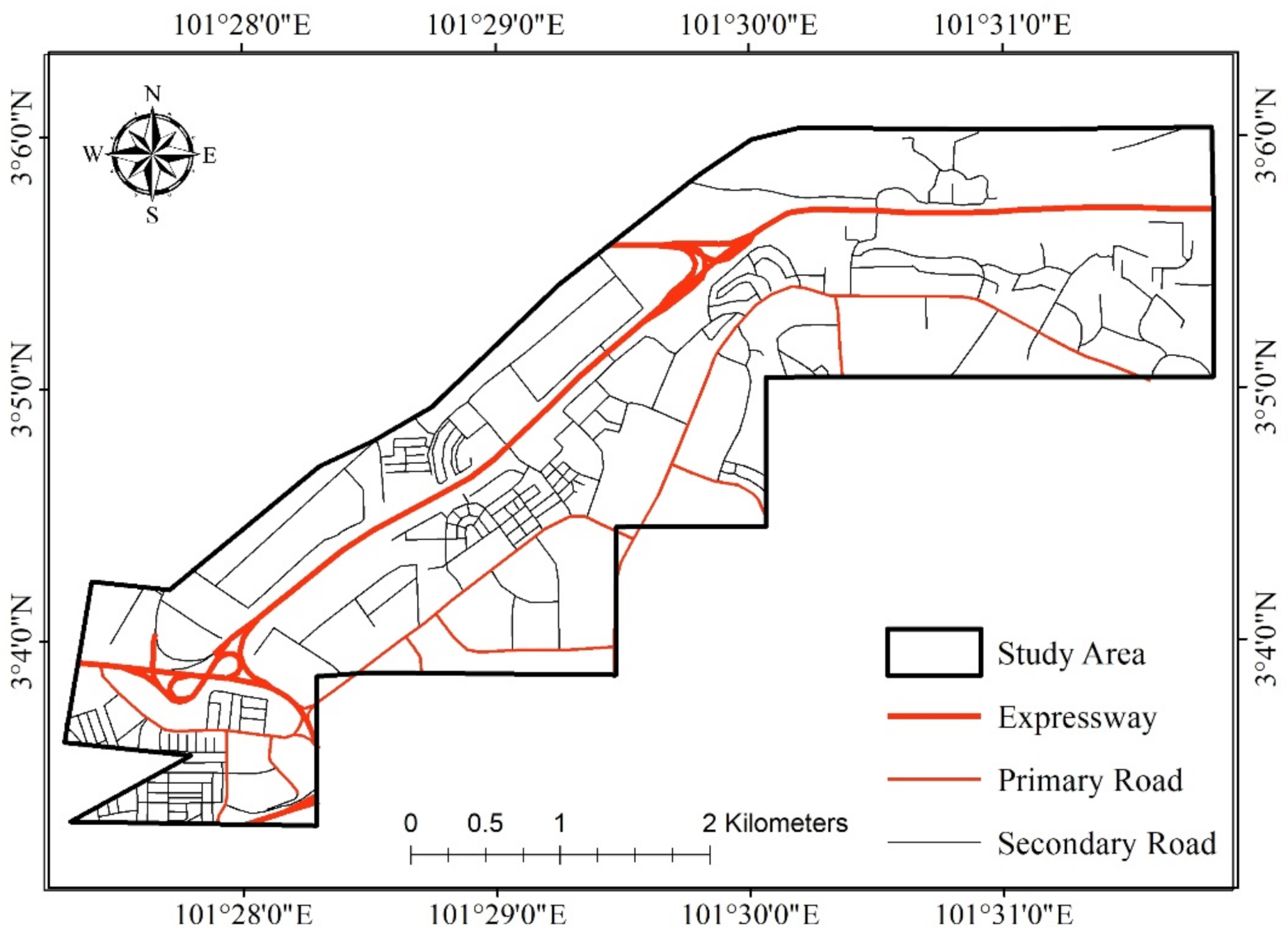
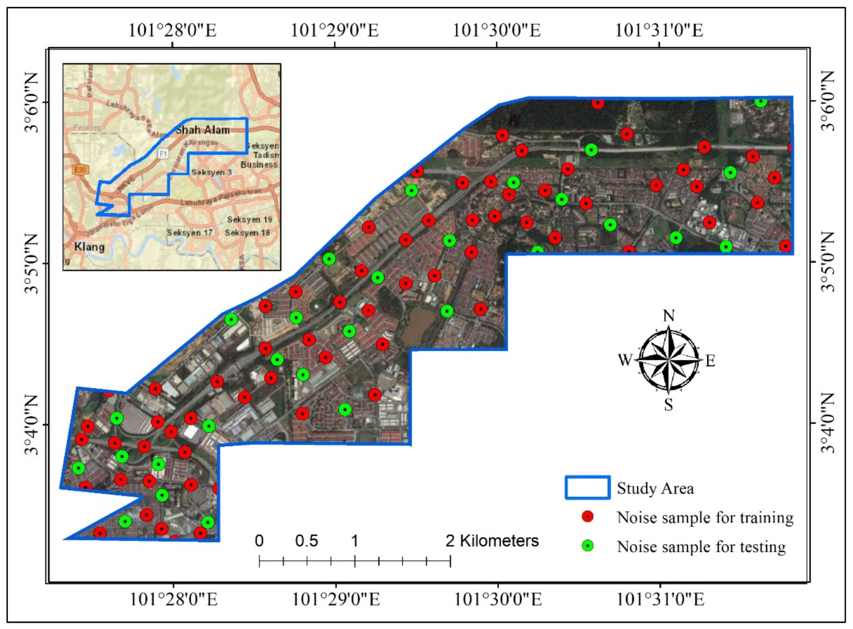
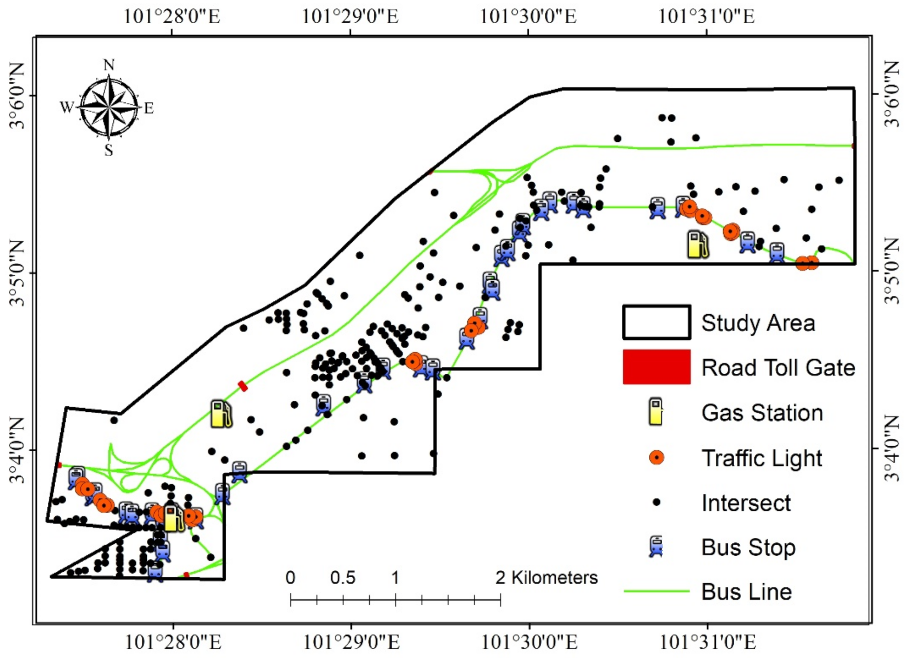
3.1. Study Area
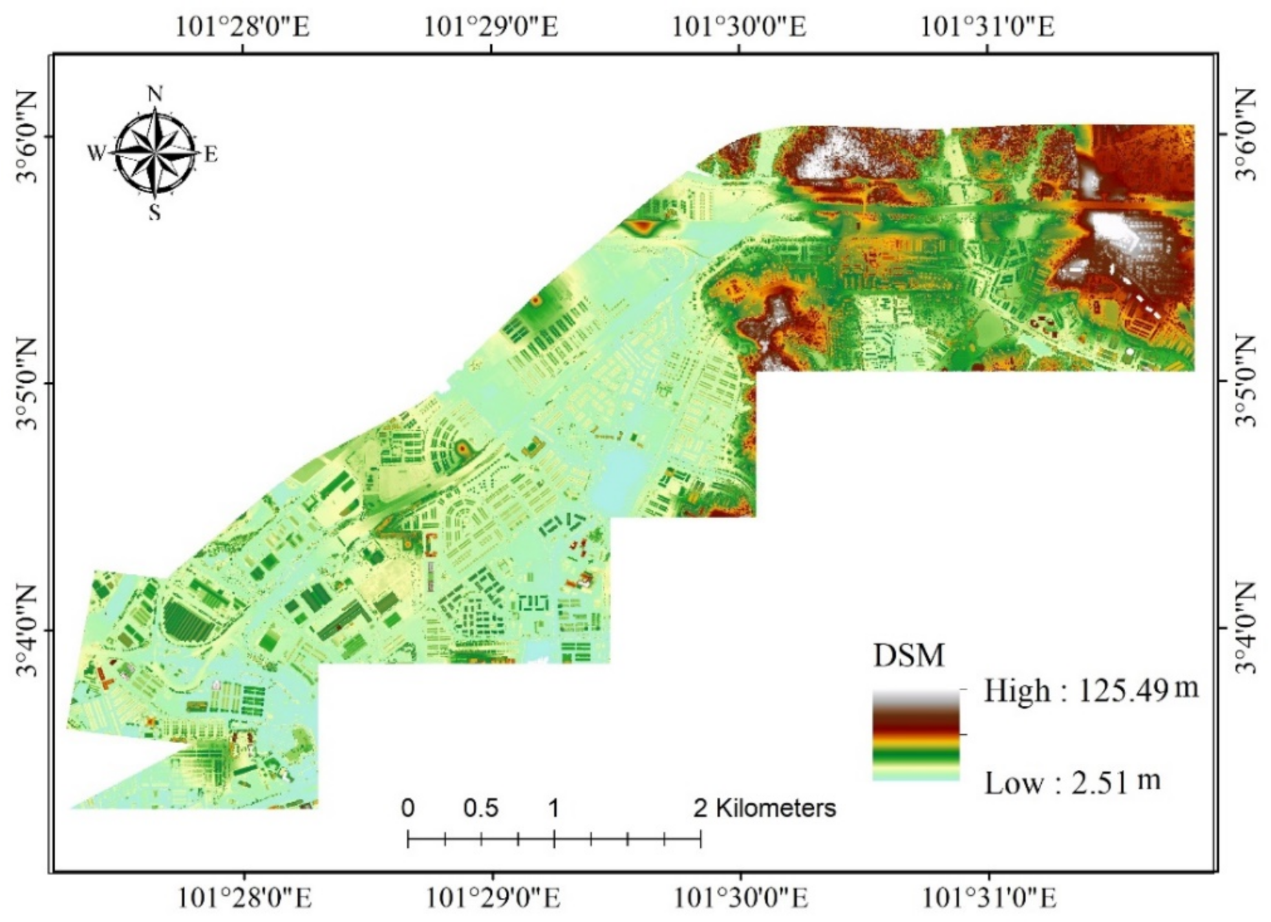
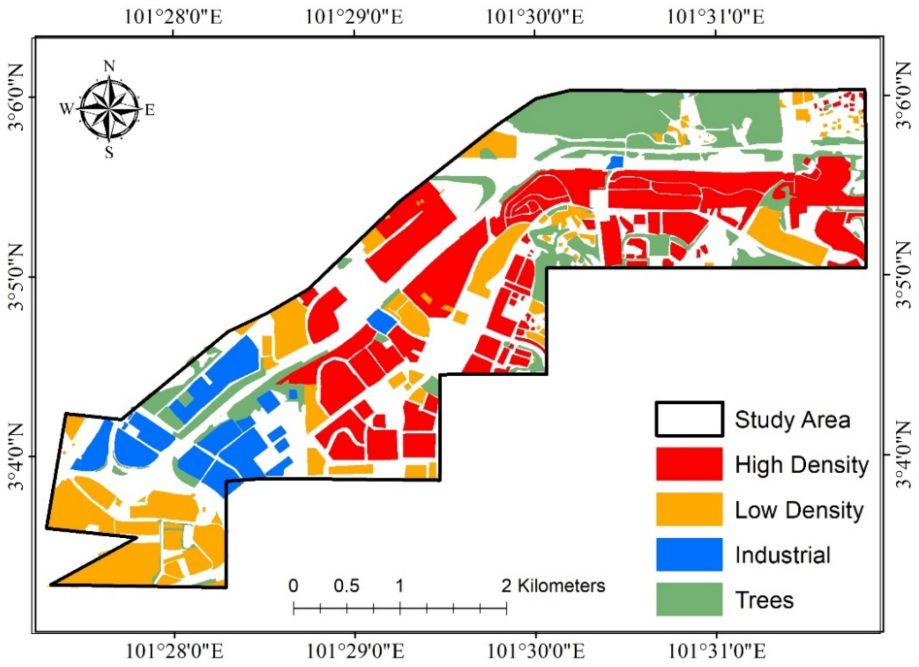
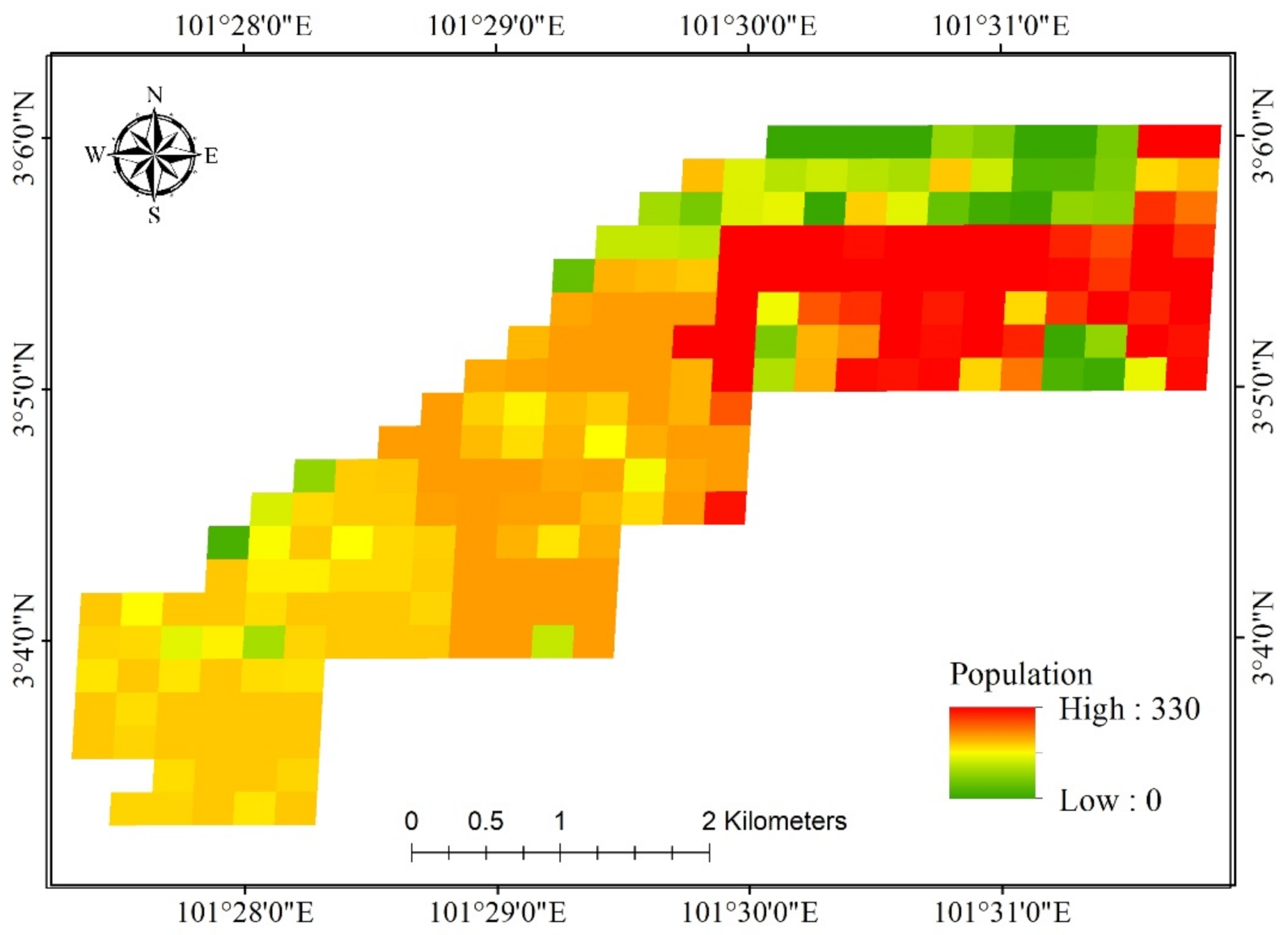
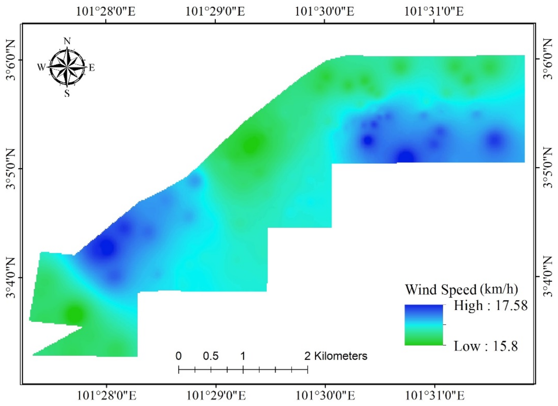
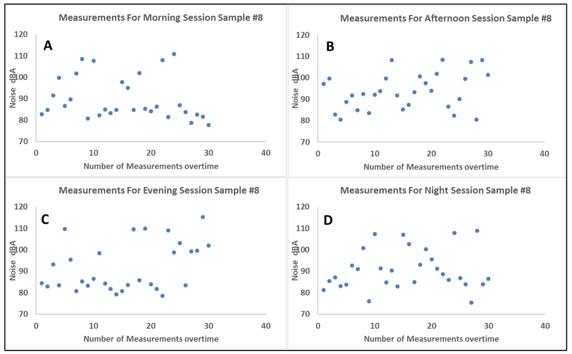
3.2. Noise Data and Predictor Variables
3.3. Data Pre-Processing
3.4. Land Use Regression Models
3.5. Model Evaluation
4. Results and Discussion
4.1. Contribution of Noise Predictors
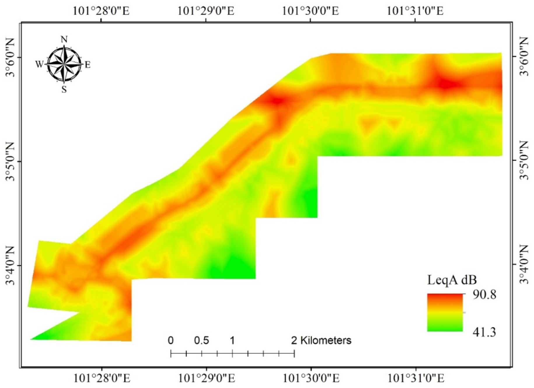
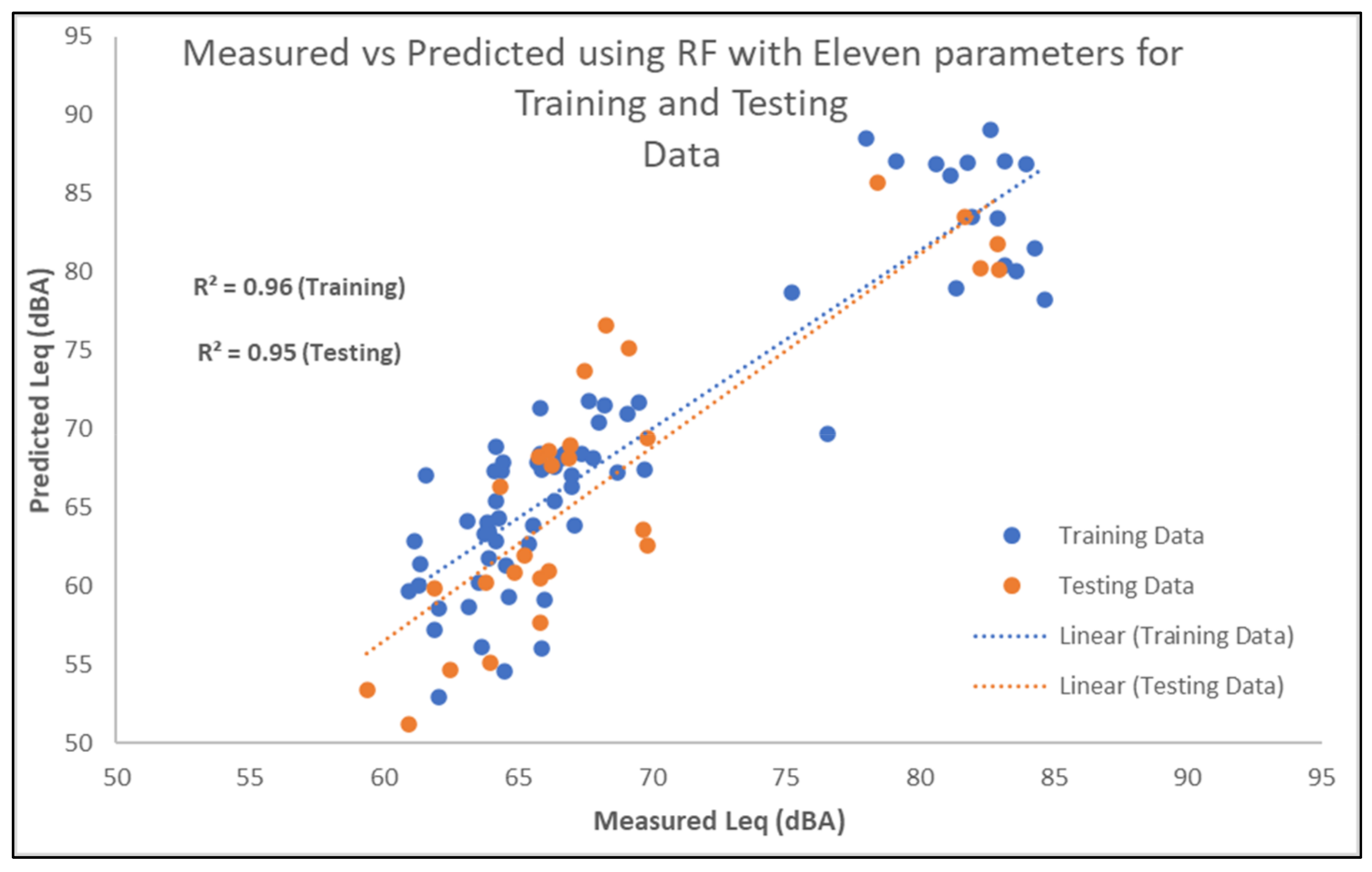
4.2. Noise Prediction
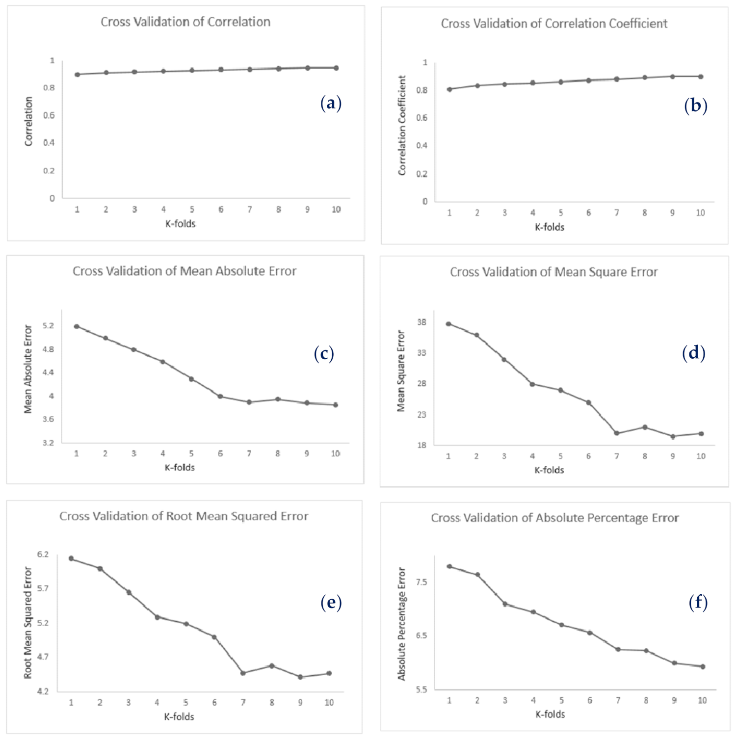
4.3. Validation of Noise Prediction Maps
5. Conclusions
Author Contributions
Funding
Institutional Review Board Statement
Informed Consent Statement
Data Availability Statement
Acknowledgments
Conflicts of Interest
Abbreviations
| Leq | Equivalent Continuous Sound Pressure |
| NKVE | New Klang Valley Expressway |
| LUR | Land Use Regression |
| GIS | Geographical Information Systems |
| LiDAR | Light Detection and Ranging |
| WHO | World Health Organization |
| DT | Decision Trees |
| RF | Random Forests |
| LR | Linear Regression |
| SVR | Support Vector Regression |
| R | Correlation |
| M | Correlation Coefficient |
| MAE | Mean Absolute Error |
| MSE | Mean Square Error |
| RMSE | Root Mean Square Error |
| MAPE | Mean Absolute Percentage Error |
| NDVI | Normalized Difference Vegetation Index |
| DSM | Digital Surface Model |
| WS | Wind Speed |
| VIF | Variance Inflation Factor |
| CFS | Correlation-Based Feature Selection |
| SVM | Support Vector Machine |
References
- Ahmed, A.A.; Pradhan, B. Vehicular traffic noise prediction and propagation modelling using neural networks and geospatial information system. Environ. Monit. Assess. 2019, 191, 1–17. [Google Scholar] [CrossRef]
- Ruiz-Padillo, A.; Ruiz, D.P.; Torija, A.J.; Ramos-Ridao, Á. Selection of suitable alternatives to reduce the environmental impact of road traffic noise using a fuzzy multi-criteria decision model. Environ. Impact. Assess. 2016, 61, 8–18. [Google Scholar] [CrossRef] [Green Version]
- Bluhm, G.; Nordling, E.; Berglind, N. Road traffic noise and annoyance-An increasing environmental health problem. Noise Health 2004, 6, 43–49. [Google Scholar]
- Moudon, A.V. Real noise from the urban environment: How ambient community noise affects health and what can be done about it. Am. J. Prev. Med. 2009, 37, 167–171. [Google Scholar] [CrossRef] [PubMed]
- Dzhambov, A.M.; Markevych, I.; Tilov, B.G.; Dimitrova, D.D. Residential greenspace might modify the effect of road traffic noise exposure on general mental health in students. Urban For. Urban Green. 2018, 34, 233–239. [Google Scholar] [CrossRef]
- Singh, D.; Kumari, N.; Sharma, P. A review of adverse effects of road traffic noise on human health. Fluct. Noise Lett. 2018, 17, 1830001. [Google Scholar] [CrossRef]
- Den Boer, L.C.; Schroten, A. Traffic noise reduction in Europe. CE Delft 2007, 14, 2057–2068. [Google Scholar]
- Steg, L.; Schuitema, G. Behavioural responses to transport pricing: A theoretical analysis. In Threats from Car Traffic to the Quality of Urban Life; Gärling, T., Steg, L., Eds.; Emerald Group Publishing Limited: Bingley, UK, 2007; pp. 347–366. [Google Scholar]
- Kawada, T. Noise and health—Sleep disturbance in adults. J. Occup. Health 2011, 53, 413–416. [Google Scholar] [CrossRef] [Green Version]
- Younes, I.; Shafiq, M.; Ghaffar, A.; Mehmood, S. Spatial Patterns of Noise Pollution and Its Effects in Lahore City; Anchor Academic Publishing: Humburg, Germany, 2007. [Google Scholar]
- Münzel, T.; Sørensen, M.; Schmidt, F.; Schmidt, E.; Steven, S.; Kröller-Schön, S.; Daiber, A. The adverse effects of environmental noise exposure on oxidative stress and cardiovascular risk. Antioxid. Redox. Signal. 2018, 28, 873–908. [Google Scholar] [CrossRef]
- Gan, W.Q.; McLean, K.; Brauer, M.; Chiarello, S.A.; Davies, H.W. Modeling population exposure to community noise and air pollution in a large metropolitan area. Environ. Res. 2012, 116, 11–16. [Google Scholar] [CrossRef]
- Licitra, G.; Teti, L.; Cerchiai, M.; Bianco, F. The influence of tyres on the use of the CPX method for evaluating the effectiveness of a noise mitigation action based on low-noise road surfaces. Transp. Res. Part D Transp. Environ. 2017, 55, 217–226. [Google Scholar] [CrossRef]
- Sandberg, U.; Ejsmont, J. Tyre/Road Noise. Reference Book; Infomex: Hard, Sweden, 2002; Available online: https://trid.trb.org/view/730140 (accessed on 3 March 2017).
- Bianco, F.; Fredianelli, L.; Lo Castro, F.; Gagliardi, P.; Fidecaro, F.; Licitra, G. Stabilization of a pu sensor mounted on a vehicle for measuring the acoustic impedance of road surfaces. Sensors 2020, 20, 1239. [Google Scholar] [CrossRef] [Green Version]
- Praticò, F.G.; Fedele, R.; Pellicano, G. Monitoring Road Acoustic and Mechanical Performance. In European Workshop on Structural Health Monitoring; Rizzo, P., Milazzo, A., Eds.; Springer: Cham, Switzerland, 2020; Volume 127, pp. 594–602. [Google Scholar]
- Teti, L.; de León, G.; Del Pizzo, A.; Moro, A.; Bianco, F.; Fredianelli, L.; Licitra, G. Modelling the acoustic performance of newly laid low-noise pavements. Constr. Build. Mater. 2020, 247, 118509. [Google Scholar] [CrossRef]
- Del Pizzo, A.; Teti, L.; Moro, A.; Bianco, F.; Fredianelli, L.; Licitra, G. Influence of texture on tyre road noise spectra in rubberized pavements. Appl. Acoust. 2020, 159, 107080. [Google Scholar] [CrossRef]
- Praticò, F.G. On the dependence of acoustic performance on pavement characteristics. Transp. Res. Part D Transp. Environ. 2014, 29, 79–87. [Google Scholar] [CrossRef]
- Praticò, F.G.; Anfosso-Lédée, F. Trends and issues in mitigating traffic noise through quiet pavements. Procedia-Soc. Behav. Sci. 2012, 53, 203–212. [Google Scholar] [CrossRef]
- de León, G.; Del Pizzo, A.; Teti, L.; Moro, A.; Bianco, F.; Fredianelli, L.; Licitra, G. Evaluation of tyre/road noise and texture interaction on rubberised and conventional pavements using CPX and profiling measurements. Road Mater. Pavement. 2020, 21, 91–102. [Google Scholar] [CrossRef] [Green Version]
- Harouvi, O.; Ben-Elia, E.; Factor, R.; de Hoogh, K.; Kloog, I. Noise estimation model development using high-resolution transportation and land use regression. J. Expo. Sci. Environ. Epidemiol. 2018, 28, 559–567. [Google Scholar] [CrossRef]
- Licitra, G.; Fredianelli, L.; Petri, D.; Vigotti, M.A. Annoyance evaluation due to overall railway noise and vibration in Pisa urban areas. Sci. Total Environ. 2016, 568, 1315–1325. [Google Scholar] [CrossRef]
- Bunn, F.; Zannin, P.H.T. Assessment of railway noise in an urban setting. Appl. Acoust. 2016, 104, 16–23. [Google Scholar] [CrossRef]
- Iglesias-Merchan, C.; Diaz-Balteiro, L.; Soliño, M. Transportation planning and quiet natural areas preservation: Aircraft overflights noise assessment in a National Park. Transp. Res. Part D Transp. Environ. 2015, 41, 1–12. [Google Scholar] [CrossRef]
- Gagliardi, P.; Fredianelli, L.; Simonetti, D.; Licitra, G. ADS-B system as a useful tool for testing and redrawing noise management strategies at Pisa Airport. Acta Acust. United Acust. 2017, 103, 543–551. [Google Scholar] [CrossRef]
- Fredianelli, L.; Bolognese, M.; Fidecaro, F.; Licitra, G. Classification of noise sources for port area noise mapping. Environments 2021, 8, 12. [Google Scholar] [CrossRef]
- Fredianelli, L.; Nastasi, M.; Bernardini, M.; Fidecaro, F.; Licitra, G. Pass-by characterization of noise emitted by different categories of seagoing ships in ports. Sustainability 2020, 12, 1740. [Google Scholar] [CrossRef] [Green Version]
- Aguilera, I.; Foraster, M.; Basagaña, X.; Corradi, E.; Deltell, A.; Morelli, X.; Künzli, N. Application of land use regression modelling to assess the spatial distribution of road traffic noise in three European cities. J. Expo. Sci. Environ. Epidemiol. 2015, 25, 97–105. [Google Scholar] [CrossRef] [PubMed]
- Manvell, D.; van Banda, E.H. Good practice in the use of noise mapping software. Appl. Acoust. 2011, 72, 527–533. [Google Scholar] [CrossRef]
- Basagana, X.; Rivera, M.; Aguilera, I.; Agis, D.; Bouso, L.; Elosua, R.; Kuenzli, N. Effect of the number of measurement sites on land use regression models in estimating local air pollution. Atmos. Environ. 2012, 54, 634–642. [Google Scholar] [CrossRef]
- Jerrett, M.; Arain, A.; Kanaroglou, P.; Beckerman, B.; Potoglou, D.; Sahsuvaroglu, T.; Giovis, C. A review and evaluation of intraurban air pollution exposure models. J. Expo. Sci. Environ. Epidemiol. 2005, 15, 185–204. [Google Scholar] [CrossRef]
- Xie, D.; Liu, Y.; Chen, J. Mapping urban environmental noise: A land use regression method. Environ. Sci. Tech. Lib. 2011, 45, 7358–7364. [Google Scholar] [CrossRef]
- Sieber, C.; Ragettli, M.S.; Brink, M.; Toyib, O.; Baatjies, R.; Saucy, A.; Röösli, M. Land use regression modeling of outdoor noise exposure in informal settlements in Western Cape, South Africa. Int. J. Environ. Res. Pub. Health 2017, 14, 1262. [Google Scholar] [CrossRef] [Green Version]
- Qing-Fang, M.; Yue-Hui, C.; Yu-Hua, P. Small-time scale network traffic prediction based on a local support vector machine regression model. Chin. Phys. B 2009, 18, 2194. [Google Scholar] [CrossRef]
- Ragettli, M.S.; Goudreau, S.; Plante, C.; Fournier, M.; Hatzopoulou, M.; Perron, S.; Smargiassi, A. Statistical modeling of the spatial variability of environmental noise levels in Montreal, Canada, using noise measurements and land use characteristics. J. Expo. Sci. Environ. Epidemiol. 2016, 26, 597–605. [Google Scholar] [CrossRef]
- Singh, D.; Nigam, S.P.; Agrawal, V.P.; Kumar, M. Vehicular traffic noise prediction using soft computing approach. J. Environ. Manage. 2016, 183, 59–66. [Google Scholar] [CrossRef] [PubMed]
- Liu, Y.; Goudreau, S.; Oiamo, T.; Rainham, D.; Hatzopoulou, M.; Chen, H.; Smargiassi, A. Comparison of land use regression and random forests models on estimating noise levels in five Canadian cities. Environ. Pollut. 2020, 256, 113367. [Google Scholar] [CrossRef]
- Garg, N.; Mangal, S.K.; Saini, P.K.; Dhiman, P.; Maji, S. Comparison of ANN and analytical models in traffic noise modeling and predictions. Acoust. Aust. 2015, 43, 179–189. [Google Scholar] [CrossRef]
- Ahn, J.; Ko, E.; Kim, E.Y. Highway traffic flow prediction using support vector regression and Bayesian classifier. In Proceedings of the International Conference on Big Data and Smart Computing (BigComp), Hong Kong, China, 18–20 January 2016. [Google Scholar]
- Crosetto, M.; Tarantola, S. Uncertainty and sensitivity analysis: Tools for GIS-based model implementation. Int. J. Geogr. Inf. Sci. 2001, 15, 415–437. [Google Scholar] [CrossRef]
- Tao, S.; Manolopoulos, V.; Rodriguez Duenas, S.; Rusu, A. Real-time urban traffic state estimation with A-GPS mobile phones as probes. J. Transp. Tech. 2012, 2, 22–31. [Google Scholar] [CrossRef] [Green Version]
- Hsieh, F.Y.; Bloch, D.A.; Larsen, M.D. A simple method of sample size calculation for linear and logistic regression. Stat. Med. 1998, 17, 1623–1634. [Google Scholar] [CrossRef] [Green Version]
- Craney, T.A.; Surles, J.G. Model-dependent variance inflation factor cutoff values. Qual. Eng. 2002, 14, 391–403. [Google Scholar] [CrossRef]
- Hall, M.A. Correlation-Based Feature Selection for Machine Learning. Ph.D. Thesis, The University of Waikato, Hamilton, New Zealand, 1999. [Google Scholar]
- Azeez, O.S.; Pradhan, B.; Shafri, H.Z. Vehicular CO emission prediction using support vector regression model and GIS. Sustainability 2018, 10, 3434. [Google Scholar] [CrossRef] [Green Version]
- Willmott, C.J.; Matsuura, K. Advantages of the mean absolute error (MAE) over the root mean square error (RMSE) in assessing average model performance. Clim. Res. 2005, 30, 79–82. [Google Scholar] [CrossRef]
- Draper, C.; Reichle, R.; de Jeu, R.; Naeimi, V.; Parinussa, R.; Wagner, W. Estimating root mean square errors in remotely sensed soil moisture over continental scale domains. Remote Sens. Environ. 2013, 137, 288–298. [Google Scholar] [CrossRef] [Green Version]
- Chai, T.; Draxler, R.R. Root mean square error (RMSE) or mean absolute error (MAE)?–Arguments against avoiding RMSE in the literature. Geosci. Model. Dev. 2014, 7, 1247–1250. [Google Scholar] [CrossRef] [Green Version]
- Verlinden, B.; Duflou, J.R.; Collin, P.; Cattrysse, D. Cost estimation for sheet metal parts using multiple regression and artificial neural networks: A case study. Int. J. Prod. Econ. 2008, 111, 484–492. [Google Scholar] [CrossRef]
- Atsalakis, G.S.; Valavanis, K.P. Surveying stock market forecasting techniques–Part II: Soft computing methods. Expert Syst. Appl. 2009, 36, 5932–5941. [Google Scholar] [CrossRef]


| Parameter (Noise Predictors) | Unit | Mean | Minimum | Maximum | Std. Dev. |
|---|---|---|---|---|---|
| Traffic volume (per 15 min) | Veh/hour | 122 | 9 | 810 | 183.66 |
| Distance from all type of roads | Meters | 67.37 | 2.11 × 10⁻⁵ | 465.12 | 65.31 |
| Distance from expressway | Meters | 426.66 | 1.74 × 10⁻⁴ | 1638.76 | 334.54 |
| Distance from primary road | Meters | 468.26 | 1.83 × 10⁻³ | 1732.76 | 366.96 |
| Distance from secondary road | Meters | 97.90 | 2.11 × 10⁻⁵ | 483.40 | 88.58 |
| Distance from area of residential high density | Meters | 402.66 | 0 | 2826.72 | 615.76 |
| Distance from area of residential low density | Meters | 190.79 | 0 | 855.10 | 175.38 |
| Distance from residential Area | Meters | 94.60 | 0 | 855.10 | 159.93 |
| Distance from industrial Area | Meters | 705.13 | 0 | 2470.92 | 568.72 |
| Distance from trees Area | Meters | 157.48 | 0 | 947.91 | 168.87 |
| DSM | Meters | 19.25 | 2.51 | 125.49 | 16.27 |
| WS | km/h | 16.62 | 15.8 | 17.58 | 0.53 |
| Distance from gas station | Meters | 1183.00 | 0 | 2726.06 | 651.41 |
| Distance from traffic lights | Meters | 780.87 | 0.58 | 1975.83 | 432.05 |
| Distance from intersect | Meters | 203.25 | 0.14 | 909.12 | 159.71 |
| Distance from road toll gate | Meters | 1010.38 | 0 | 2239.69 | 513.18 |
| Distance from bus stop | Meters | 528.22 | 0.083 | 1736.24 | 334.74 |
| Distance from bus line | Meters | 214.94 | 1.86 × 10⁻⁴ | 946.33 | 161.00 |
| Noise Predictor | Multiple R-Square | VIF |
|---|---|---|
| Traffic volume | 0.64 | 2.78 |
| All type of roads | 0.25 | 1.33 |
| Expressway | 0.82 | 5.64 |
| Primary road | 0.89 | 9.15 |
| Secondary road | 0.37 | 1.59 |
| Area of residential high density | 0.82 | 5.49 |
| Area of residential low density | 0.63 | 2.71 |
| Residential area | 0.71 | 3.45 |
| Industrial area | 0.70 | 3.28 |
| Trees area | 0.49 | 1.96 |
| DSM | 0.53 | 2.14 |
| WS | 0.74 | 3.87 |
| Gas station | 0.75 | 4.06 |
| Traffic lights | 0.71 | 3.47 |
| Intersect | 0.61 | 2.56 |
| Tool road | 0.65 | 2.82 |
| Bus stop | 0.89 | 8.96 |
| Bus line | 0.72 | 3.52 |
| Method | LR | DT | RF | SVM | |||||
|---|---|---|---|---|---|---|---|---|---|
| Evaluation | Training | Testing | Training | Testing | Training | Testing | Training | Testing | |
| R | 0.93 | 0.91 | 0.92 | 0.91 | 0.95 | 0.93 | 0.94 | 0.92 | |
| R2 | 0.864 | 0.83 | 0.84 | 0.82 | 0.90 | 0.866 | 0.88 | 0.85 | |
| MAE | 3.88 | 4.49 | 4.04 | 4.62 | 3.30 | 4.46 | 3.81 | 4.80 | |
| MSE | 23.12 | 32.73 | 26.82 | 29.13 | 17.48 | 27.26 | 20.93 | 28.76 | |
| RMSE | 4.81 | 5.72 | 5.18 | 5.40 | 4.18 | 5.22 | 4.58 | 5.36 | |
| MAPE | 5.72 | 7.26 | 6.15 | 7.11 | 4.86 | 7.06 | 5.55 | 7.43 | |
| Method | LR | DT | RF | SVM | |||||
|---|---|---|---|---|---|---|---|---|---|
| Evaluation | Training | Testing | Training | Testing | Training | Testing | Training | Testing | |
| R | 0.94 | 0.94 | 0.95 | 0.94 | 0.96 | 0.95 | 0.94 | 0.94 | |
| R2 | 0.88 | 0.88 | 0.90 | 0.88 | 0.92 | 0.90 | 0.89 | 0.88 | |
| MAE | 3.66 | 4.46 | 3.36 | 4.26 | 2.99 | 3.86 | 3.64 | 4.30 | |
| MSE | 20.25 | 22.91 | 17.99 | 23.35 | 13.99 | 19.96 | 19.10 | 23.95 | |
| RMSE | 4.50 | 4.79 | 4.24 | 4.83 | 3.47 | 4.47 | 4.37 | 4.89 | |
| MAPE | 5.45 | 6.28 | 5.05 | 6.42 | 4.37 | 5.94 | 5.35 | 6.65 | |
Publisher’s Note: MDPI stays neutral with regard to jurisdictional claims in published maps and institutional affiliations. |
© 2021 by the authors. Licensee MDPI, Basel, Switzerland. This article is an open access article distributed under the terms and conditions of the Creative Commons Attribution (CC BY) license (https://creativecommons.org/licenses/by/4.0/).
Share and Cite
Adulaimi, A.A.A.; Pradhan, B.; Chakraborty, S.; Alamri, A. Traffic Noise Modelling Using Land Use Regression Model Based on Machine Learning, Statistical Regression and GIS. Energies 2021, 14, 5095. https://doi.org/10.3390/en14165095
Adulaimi AAA, Pradhan B, Chakraborty S, Alamri A. Traffic Noise Modelling Using Land Use Regression Model Based on Machine Learning, Statistical Regression and GIS. Energies. 2021; 14(16):5095. https://doi.org/10.3390/en14165095
Chicago/Turabian StyleAdulaimi, Ahmed Abdulkareem Ahmed, Biswajeet Pradhan, Subrata Chakraborty, and Abdullah Alamri. 2021. "Traffic Noise Modelling Using Land Use Regression Model Based on Machine Learning, Statistical Regression and GIS" Energies 14, no. 16: 5095. https://doi.org/10.3390/en14165095
APA StyleAdulaimi, A. A. A., Pradhan, B., Chakraborty, S., & Alamri, A. (2021). Traffic Noise Modelling Using Land Use Regression Model Based on Machine Learning, Statistical Regression and GIS. Energies, 14(16), 5095. https://doi.org/10.3390/en14165095