Article

Estimation of Functional Form of Time-Dependent Heat Transfer Coefficient Using an Accurate and Robust Parameter Estimation Approach: An Inverse Analysis

1
Zienkiewicz Centre for Computational Engineering, Faculty of Science and Engineering, Swansea University, Swansea SA1 8EN, UK
2
Department of Mechanical Engineering, University of Canterbury, Private Bag 4800, Christchurch 8140, New Zealand
*
Author to whom correspondence should be addressed.
Energies 2021, 14(16), 5073; https://doi.org/10.3390/en14165073
Submission received: 14 July 2021 / Revised: 11 August 2021 / Accepted: 12 August 2021 / Published: 18 August 2021
(This article belongs to the Special Issue Mathematical Modelling of Energy Systems and Fluid Machinery 2022)

Abstract

:
This paper presents a numerical method to address function estimation problems in inverse heat transfer problems using parameter estimation approach without prior information on the functional form of the variable to be estimated. Using an inverse analysis, the functional form of a time-dependent heat transfer coefficient is estimated efficiently and accurately. The functional form of the heat transfer coefficient is assumed unknown and the inverse heat transfer problem should be treated using a function estimation approach by solving sensitivity and adjoint problems during the minimization process. Based on proposing a new sensitivity matrix, however, the functional form can be estimated in an accurate and very efficient manner using a parameter estimation approach without the need for solving the sensitivity and adjoint problems and imposing extra computational cost, mathematical complexity, and implementation efforts. In the proposed sensitivity analysis scheme, all sensitivity coefficients can be computed in only one direct problem solution at each iteration. In this inverse heat transfer problem, the body shape is irregular and meshed using a body-fitted grid generation method. The direct heat conduction problem is solved using the finite-difference method. The steepest-descent method is used as a minimization algorithm to minimize the defined objective function and the termination of the minimization process is carried out based on the discrepancy principle. A test case with three different functional forms and two different measurement errors is considered to show the accuracy and efficiency of the used inverse analysis.

1. Introduction

In a heat transfer problem, the accuracy of thermophysical properties and boundary conditions is critical to obtain an accurate numerical simulation. As a boundary condition, convective heat transfer depends on different parameters such as time, surface geometry, and surface temperature, to name a few. The accurate determination of the convective heat transfer coefficient is a difficult task as convection is a very complicated phenomenon and expensive experiments with sophisticated instruments are required to appropriately unravel its dynamics [1].
The advent of high-speed and high-capacity computers and the development of different regularization methods over the past decades have played significant roles in successful applications of numerical inverse methods, as inexpensive alternatives to costly and time-consuming experiments with sophisticated instruments, to appropriately estimate unknown heat transfer quantities such as the heat transfer coefficient [2,3,4,5,6,7,8,9,10]. Inverse heat transfer problems are mathematically challenging problems because they are ill-posed and the accuracy of the estimation of an unknown quantity is very sensitive to measurement errors [11,12,13]. If the unknown quantity to be estimated (in this study, the heat transfer coefficient) can be expressed as a constant parameter [14,15] or represented by a few parameters [16], a parameter estimation approach may be used to estimate the parameters thereby estimating the unknown quantity. However, a function estimation approach should be used to estimate the unknown functional form of the unknown quantity when there is no information available on the functional form of the unknown quantity. In the function estimation approach, the sensitivity and adjoint problems are required to obtain the gradient of objective function with respect to unknown functional form which impose additional mathematical developments and computational costs on the inverse analysis. In this study, based on the numerical procedure employed in [17], a two-dimensional transient inverse heat conduction problem is considered. The thermophysical properties are assumed constant, the geometry of heat-conducting body is irregular, and the body is subject to Neumann and Robin boundary conditions at its boundary surface parts. Using the parameter estimation approach initially developed in [17] for the estimation of unknown functional form of a time-dependent heat flux (a boundary condition of second kind) imposed at a boundary surface, here the unknown functional form of a time-dependent heat transfer coefficient(a third-kind boundary condition) is estimated efficiently and accurately without involving the solution of the sensitivity and adjoint problems. Thus, the mathematical development effort and the computational cost are reduced significantly.
To do so, the heat-conducting body (the physical domain) is mapped onto a regular computational domain in order to take advantage of the ease of implementation of the finite-difference method to explicitly solve the transient heat conduction equation and the associated boundary conditions. As the body shape is irregular, a body-fitted (elliptic) grid generation method is used to mesh the irregular domain which makes the proposed method general and applicable to any irregular domain as long as it can be mapped onto a regular computational domain. Using the chain rule to relate the temperature at sensor place and the time-dependent heat transfer coefficient applied on the part of the body boundary, explicit expressions are derived to compute sensitivity coefficients during the solution of the transient heat conduction equation without the need for solving the sensitivity and adjoint equations. The steepest-descent method, as an iterative regularization method, with a stopping criterion specified by discrepancy principle is used to minimize the objective function and reach the solution accurately. A test case with three complicated functional forms of timewise variation of the heat transfer coefficient is presented to reveal the accuracy, efficiency, and robustness of the inverse analysis. Moreover, two different measurement errors are considered. It is shown that the inverse analysis is not strongly affected by the errors involved in the temperature measurements and the unknown functional forms of the timewise variation of the heat transfer coefficient can be recovered with excellent accuracy. As stated before, the objective of this study is to present a parameter estimation approach to estimate the unknown functional form of a time-dependent heat transfer coefficient efficiently and accurately.

2. Governing Equation
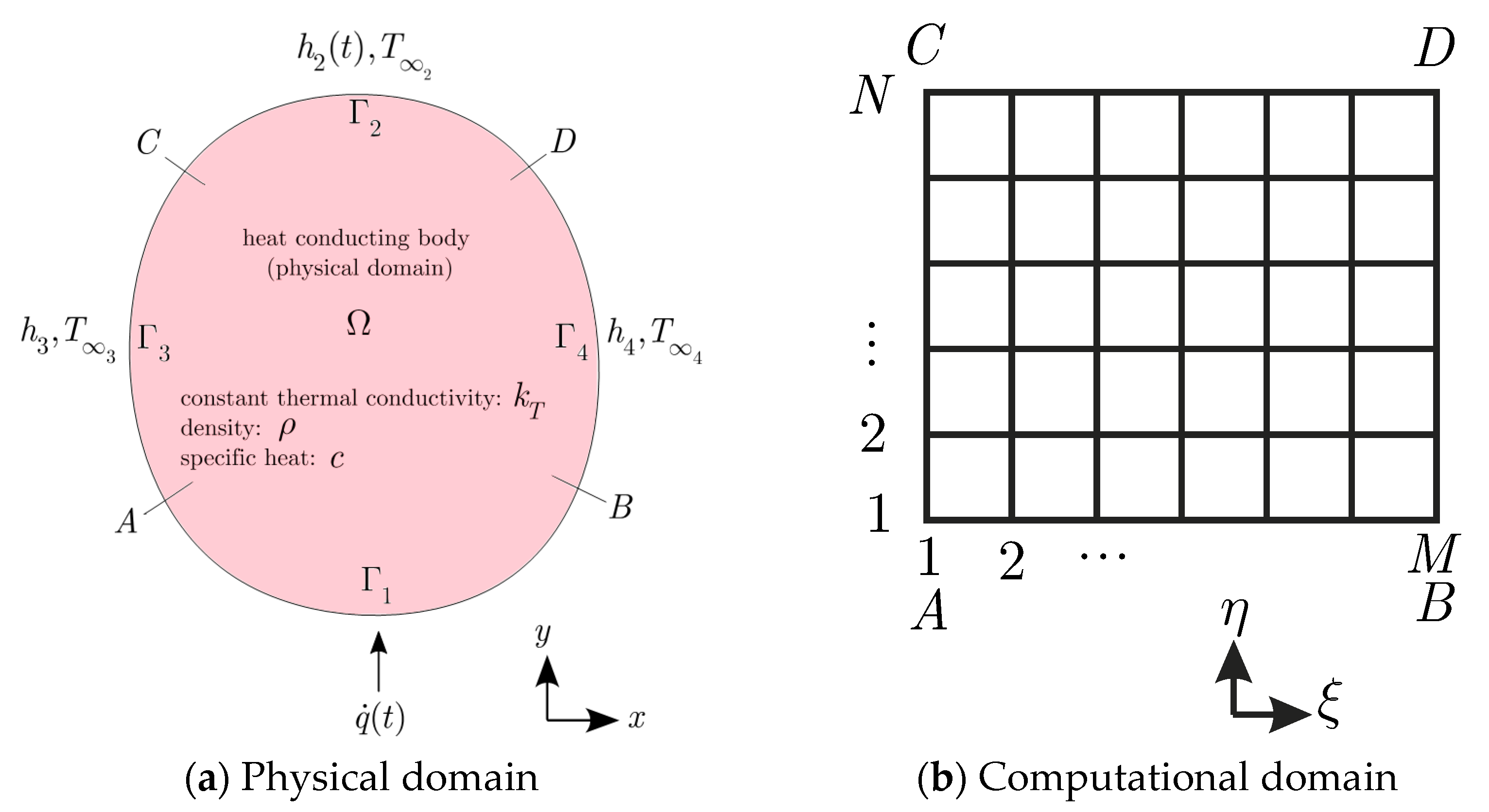
The body shown in Figure 1a is initially at the temperature T 0 . At time t > 0 , it is exposed to a time-dependent heat flux q ˙ ( t ) at boundary surface Γ 1 and convective heat transfer on boundary surfaces Γ i , i = 2 , 3 , 4 with corresponding heat transfer coefficients h 2 ( t ) , h 3 , and h 4 and surrounding temperatures T i , i = 2 , 3 , 4 . The thermal conductivity, density, and specific heat of the body are k T , ρ , and c , respectively.
The governing equation for a two-dimensional transient heat conduction problem with no heat generation can be expressed as [17,18]
k T ( 2 T ( x , y , t ) x 2 + 2 T ( x , y , t ) y 2 ) = ρ c T ( x , y , t ) t   in   physical   domain   Ω ( x , y )
with the boundary and initial conditions
T ( x , y , t ) n 1 = q ˙ ( t ) k T   on   boundary   surface   Γ 1 ( x , y )
T ( x , y , t ) n 2 = h 2 ( t ) k T ( T Γ 2 ( x , y , t ) - T 2 )   on   boundary   surface   Γ 2 ( x , y )
T ( x , y , t ) n i = h i k T ( T Γ i ( x , y , t ) - T i )   on   boundary   surface   Γ i ( x , y ) , i = 3 , 4
T ( x , y , 0 ) = T 0 ( x , y )   in   physical   domain   Ω ( x , y )
where t is the time. Since the heat-conducting body is irregular, it (the x and y physical domain) can be mapped onto a regular one (the ξ and η computational domain). The elliptic grid generation method is employed to generate a grid over the physical domain. Then the heat conduction equation and its associated boundary and initial conditions can be transformed from the ( x , y , t ) to the ( ξ , η , t ) variables [12,18]. The transformation results in
( α 2 T ( ξ , η , t ) ξ 2 2 β 2 T ( ξ , η , t ) ξ η + γ 2 T ( ξ , η , t ) η 2 J 2 + ( 2 ξ ) T ( ξ , η , t ) ξ + ( 2 η ) T ( ξ , η , t ) η ) = ρ c k T T ( ξ , η , t ) t
where 2 ξ = P ( ξ , η ) and 2 η = Q ( ξ , η ) are grid control functions. If P ( ξ , η ) = Q ( ξ , η ) = 0 , then a smooth grid over the physical domain is obtained. Therefore, Equation (6) becomes
( α 2 T ( ξ , η , t ) ξ 2 2 β 2 T ( ξ , η , t ) ξ η + γ 2 T ( ξ , η , t ) η 2 J 2 ) = ρ c k T T ( ξ , η , t ) t   in   1 < ξ < M , 1 < η < N ,   for   t > 0
where
α = x η 2 + y η 2
β = x ξ x η + y ξ y η
γ = x ξ 2 + y ξ 2
J = x ξ y η x η y ξ ( Jacobian   of   transformation )  
The transformed boundary and initial conditions can be expressed as
( 1 J γ ( γ T ( ξ , η , t ) η β T ( ξ , η , t ) ξ ) ) Γ 1 = q ˙ ( t ) k T   at   1 < ξ < M , η = 1 ,   for   t > 0  
( 1 J γ ( γ T ( ξ , η , t ) η β T ( ξ , η , t ) ξ ) ) Γ 2 = h 2 ( t ) k T ( T ( ξ , η , t ) T 2 )   at   1 < ξ < M , η = N ,   for   t > 0
( 1 J α ( α T ( ξ , η , t ) ξ β T ( ξ , η , t ) η ) ) Γ 3 = h 3 k T ( T ( ξ , η , t ) T 3 )   at   1 < η < N , ξ = 1 ,   for   t > 0  
( 1 J α ( α T ( ξ , η , t ) ξ β T ( ξ , η , t ) η ) ) Γ 4 = h 4 k T ( T ( ξ , η , t ) T 4 )   at   1 < η < N , ξ = M ,   for   t > 0  
T ( ξ , η , 0 ) = T 0 * ( ξ , η )   in   1 < ξ < M , 1 < η < N ,   for   t = 0
where the initial condition T 0 ( x , y ) is rewritten as T 0 * ( ξ , η ) in terms of the variables ξ and η . Now the finite-difference method can be employed to discretize the derivatives present in the above equations in the regular computational domain, as follows (assuming Δ ξ = Δ η = 1 )
f ξ = 1 2 ( f i + 1 , j f i 1 , j )
f η = 1 2 ( f i , j + 1 f i , j 1 )
f ξ ξ = f i + 1 , j 2 f i , j + f i 1 , j
f η η = f i , j + 1 2 f i , j + f i , j 1
f ξ η = 1 4 ( f i + 1 , j + 1 f i 1 , j + 1 f i + 1 , j 1 + f i 1 , j 1 )
where f x , y , T . One-sided forward and one-sided backward relations are used to discretize the boundary condition equations. The explicit method can be used to solve the resulting transient heat conduction equation, Equation (7). Using forward-time-central-space (FTCS) discretization and the relations in Equation (14), we get
1 J 2 ( α ( T i + 1 , j n 2 T i , j n + T i 1 , j n ) 2 β 1 4 ( T i + 1 , j + 1 n T i 1 , j + 1 n T i + 1 , j 1 n + T i 1 , j 1 n ) + γ ( T i , j + 1 n 2 T i , j n + T i , j 1 n ) ) = ρ c k T T i , j n + 1 T i , j n Δ t ,   i = 2 , , M 1 , j = 2 , , N 1   for   t > 0
where Δ t is the time step. Taking into account the stability criterion, the time-marching procedure can be used to solve Equation (15) and obtain T i , j n + 1 . That is, the nodal temperatures at the time level n + 1 , T i , j n + 1 , can be determined from the knowledge of nodal temperatures at the previous time level n , T i , j n , as follows
T i , j n + 1 = T i , j n + k T Δ t ρ c J 2 ( α ( T i + 1 , j n 2 T i , j n + T i 1 , j n ) 2 β 1 4 ( T i + 1 , j + 1 n T i 1 , j + 1 n T i + 1 , j 1 n + T i 1 , j 1 n ) + γ ( T i , j + 1 n 2 T i , j n + T i , j 1 n ) )

3. The Inverse Analysis

3.1. Objective Function

The inverse heat transfer problem of interest deals with the estimation of the time-dependent heat transfer coefficient h 2 ( t ) applied at the time t i and at the surface Γ 2 , h 2 ( t i ) , i = 1 , , r ( r is the number of time steps) using the transient readings of a single sensor S placed at the point ( S i , S j ) inside the heat conducting body. In inverse analysis, the aim is to minimize the mismatch between the estimated temperatures at the sensor place, T e ( S i , S j , t i ) , computed from the solution of the direct transient heat conduction problem using the estimated heat transfer coefficient h 2 ( t i ) and the measured temperatures T m ( S i , S j , t i ) over the time domain 0 < t < t r . This can be mathematically expressed as a least-squares minimization as follows
min   { J h 2   at   Γ 2 : = T e ( S i , S j , t ) T m ( S i , S j , t ) 2 : Equation ( 1 )   in   Ω ,   BCs   and   IC   in   Equations   ( 2 ) ( 5 ) }
where h 2 = [ h 2 ( t 1 ) , h 2 ( t 2 ) , h 2 ( t 3 ) , , h 2 ( t r ) ] T . Therefore, the objective function can be expressed as
J = i = 1 r [ T e ( S i , S j , t i ) T m ( S i , S j , t i ) ] 2

3.2. Sensitivity Analysis

The calculation of the gradient of the objective function J defined by Equation (18) with respect to h 2 ( t i ) , i = 1 , , r is required in gradient-based minimization methods. Therefore, it can be written
J h 2 ( t i ) = 2 i = 1 r [ T e ( S i , S j , t i ) T m ( S i , S j , t i ) ] T e ( S i , S j , t i ) h 2 ( t i )
The sensitivity coefficients T e ( S i , S j , t i ) h 2 ( t i ) ( i = 1 , , r , i = 1 , , r ) can be explicitly expressed using the chain rule (using the constant thermal conductivity k T ) as follows
T e ( S i , S j , t i ) h 2 ( t i ) = T e ( S i , S j , t i ) k T h 2 ( t i ) k T
The expression in the numerator of Equation (20), T e ( S i , S j , t i ) k T , can be obtained by taking derivative of T i , j n + 1 in Equation (16) with respect to k T , as follows
T e n + 1 ( S i , S j , t i ) k T = Δ t ρ c J 2 ( α ( T S i + 1 , S j n 2 T S i , S j n + T S i 1 , S j n ) 2 β 1 4 ( T S i + 1 , S j + 1 n T S i 1 , S j + 1 n T S i + 1 , S j 1 n + T S i 1 , S j 1 n ) + γ ( T S i , S j + 1 n 2 T S i , S j n + T S i , S j 1 n ) )
The expression in the denominator of Equation (20), T e ( S i , S j , t i ) k T , can be obtained from the boundary condition involving the heat transfer coefficient h 2 ( t ) , Equation (9), as follows
( 1 J γ ( γ T ( ξ , η , t ) η β T ( ξ , η , t ) ξ ) ) Γ 2 = h 2 ( t ) k T ( T ( ξ , η , t ) T 2 )  
therefore, we get
h 2 ( t i ) k T = 1 T ( ξ , η , t ) T 2 ( 1 J γ ( γ T ( ξ , η , t ) η β T ( ξ , η , t ) ξ ) ) Γ 2
where the terms T ξ , T η , J , γ and β are computed using the finite-difference expressions associated with the surface Γ 2 . That is,
f ξ = 1 2 ( f i + 1 , N f i 1 , N )
f η = 1 2 ( 3 f i , N 4 f i , N 1 + f i , N 2 )
where f x , y , T . Therefore, the sensitivity coefficients in Equation (20) can be calculated by dividing the term in Equation (21) by the one in Equation (23).
T e ( S i , S j , t i ) h 2 ( t i ) = 1 ( 1 T ( ξ , η , t ) T 2 ( 1 J γ ( γ T ( ξ , η , t ) η β T ( ξ , η , t ) ξ ) ) Γ 2 ) t i Δ t ρ c J 2 ( α ( T S i + 1 , S j t i 2 T S i , S j t i + T S i 1 , S j t i ) 2 β 1 4 ( T S i + 1 , S j + 1 t i T S i 1 , S j + 1 t i T S i + 1 , S j 1 t i + T S i 1 , S j 1 t i ) + γ ( T S i , S j + 1 t i 2 T S i , S j t i + T S i , S j 1 t i ) )
It can be seen that all sensitivity coefficients T e ( S i , S j , t i ) h 2 ( t i ) can be computed during the transient solution of the direct heat conduction equation. The sensitivity matrix Ja can be explicitly written as
J a h 2 ( t ) = [ T e ( S i , S j , t 1 ) h 2 ( t 1 ) T e ( S i , S j , t 1 ) h 2 ( t 2 ) T e ( S i , S j , t 1 ) h 2 ( t 3 ) T e ( S i , S j , t 1 ) h 2 ( t r ) T e ( S i , S j , t 2 ) h 2 ( t 1 ) T e ( S i , S j , t 2 ) h 2 ( t 2 ) T e ( S i , S j , t 2 ) h 2 ( t 3 ) T e ( S i , S j , t 2 ) h 2 ( t r ) T e ( S i , S j , t 3 ) h 2 ( t 1 ) T e ( S i , S j , t 3 ) h 2 ( t 2 ) T e ( S i , S j , t 3 ) h 2 ( t 3 ) T e ( S i , S j , t 3 ) h 2 ( t r ) T e ( S i , S j , t r ) h 2 ( t 1 ) T e ( S i , S j , t r ) h 2 ( t 2 ) T e ( S i , S j , t r ) h 2 ( t 3 ) T e ( S i , S j , t r ) h 2 ( t r ) ] r × r
We know that the temperature estimated at any time is independent of a yet-to-occur future heat transfer coefficient component [11,19] which gives rise to a lower-triangular sensitivity matrix. That is, for i > i (the terms above the main diagonal of the sensitivity matrix), T e ( S i , S j , t i ) h 2 ( t i ) = 0 . Thus, we get
J a h 2 ( t ) = [ T e ( S i , S j , t 1 ) h 2 ( t 1 ) 0 0 0 T e ( S i , S j , t 2 ) h 2 ( t 1 ) T e ( S i , S j , t 2 ) h 2 ( t 2 ) 0 0 T e ( S i , S j , t 3 ) h 2 ( t 1 ) T e ( S i , S j , t 3 ) h 2 ( t 2 ) T e ( S i , S j , t 3 ) h 2 ( t 3 ) 0 T e ( S i , S j , t r ) h 2 ( t 1 ) T e ( S i , S j , t r ) h 2 ( t 2 ) T e ( S i , S j , t r ) h 2 ( t 3 ) T e ( S i , S j , t r ) h 2 ( t r ) ] r × r

3.3. The Steepest-Descent Method

The steepest-descent optimization method is used in this study to minimize the objective function given by Equation (18) by searching along the direction of steepest descent   d ( k ) using a search step length   β ( k ) .
h 2 ( k + 1 ) = h 2 ( k ) + β ( k ) d ( k )
The negative of the gradient direction   J ( k ) denotes the direction of steepest descent d ( k ) . Thus,
d ( k ) = J ( k )
In the expression h 2 ( k + 1 ) = h 2 ( k ) + β ( k ) d ( k ) = h 2 ( k ) β ( k ) J ( k ) , the search step-length β ( k ) > 0 is given as follows [12]
β ( k ) = [ J a ( k ) d ( k ) ] T [ T e T m ] [ J a ( k ) d ( k ) ] T [ J a ( k ) d ( k ) ]

Optimization Algorithm

The proposed numerical procedure to estimate the time-dependent heat transfer coefficient at the boundary surface Γ 2 , h 2 ( t ) , can be summarized as follows:
  • Measure the temperatures at the sensor place S S i , S j and the time t i ( i = 1 , , r ), T m ( S i , S j , t i ) .
  • Solve the direct problem to obtain the temperature values at the sensor place and the time t i ( i = 1 , , r ), T e ( S i , S j , t i ) , through solving Equations (7)–(13).
  • Compute the objective function value ( J ( k ) ) using Equation (18).
  • If value of the objective function obtained in step 3 is less than the specified stopping criterion, the optimization is finished. Otherwise, go to step 5.
  • Compute the sensitivity matrix J a h 2 ( t ) from Equation (26), the gradient direction J ( k ) from Equation (19), the direction of descent d ( k ) from Equation (28), and the search step-length β ( k ) from Equation (29).
  • Update h 2 from Equation (27) and set the next iteration ( k = k + 1 ) and return to the step 2.

3.4. Stopping Criterion

The minimization process can be terminated if
J ( k ) < ε
where ε is chosen based on obtaining stable and appropriate results. In this study, when there are no measurement errors, ε = 10 6 . However, if the temperature measurements contain errors, then the discrepancy principle is used to stop the iterative procedure and obtain stable results. In this case,
ε = r σ 2
where σ is the standard deviation of the measurement errors [17] and is assumed constant in this study ( σ = 0.001 and σ = 0.005 ). Here, the measured temperatures containing random errors, T meas ( S i , S j , t i ) , ( i = 1 , , r ) , are generated by adding an error term ω σ to the exact temperatures T exact ( S i , S j , t i ) to give
T meas ( S i , S j , t i ) = T exact ( S i , S j , t i ) + ω σ
where ω is a random variable with normal (Gaussian) distribution, zero mean, and unitary standard deviation. Assuming 99% confidence for the measured temperature, ω lies in the range 2.576 ω 2.576   and it is randomly generated by using MATLAB.

4. Results

A test case with three different complicated functional forms of variation of the heat transfer coefficient with time is presented to investigate the accuracy, efficiency, and robustness of the proposed sensitivity analysis method to estimate the time-dependent heat transfer coefficient on part of the boundary of a heat conducting body. Initially the heat transfer coefficient is assumed to be known, the transient heat conduction problem is then solved to calculate the temperature at the sensor place at times t i ( i = 1 , , r ). Then, the calculated temperatures are used as 
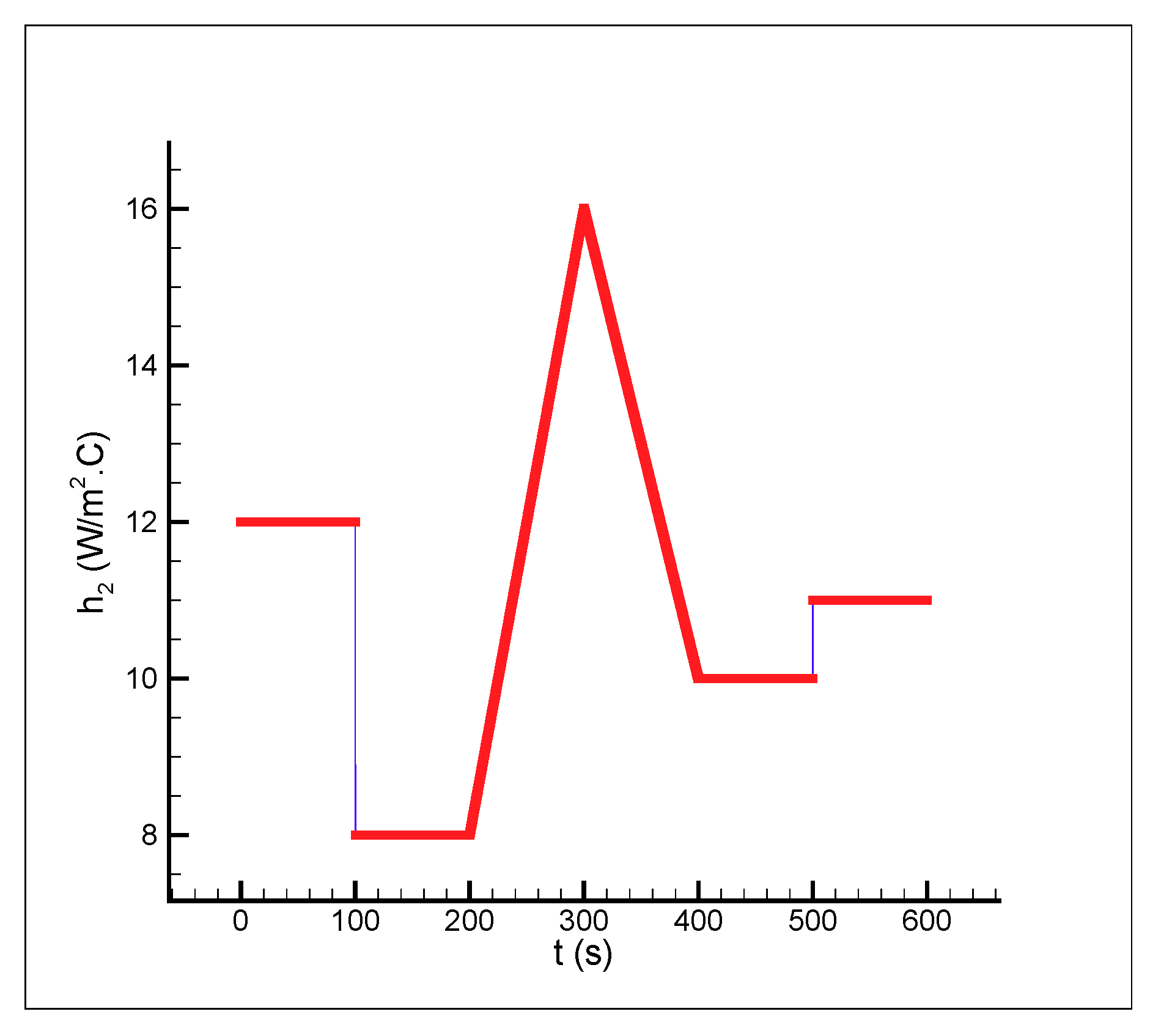
simulated measured ones to recover the initially used heat transfer coefficient. The three different forms of timewise variation of the heat transfer coefficient considered are as follows (Figure 2, Figure 3 and Figure 4)
h 2 ( 1 ) ( t ) = { 12 , 0 t < 100 s 8 , 100 t < 200 s 16 8 300 200 ( t 200 ) + 8 , 200 t 300 s 10 16 400 300 ( t 300 ) + 16 , 300 < t 400 s 10 , 400 < t 500 s 11 , 500 < t 600 s
h 2 ( 2 ) ( t ) = 10 + log ( t 0.5 ) sin ( t 6 ) + t 0.45
and h 2 ( 3 ) ( t ) which is an arbitrary waveform generated in MATLAB used here to model the variation of the heat transfer coefficient with time.
Assuming the heat conducting body is made of stainless steel (type 304), the numerical values of the coefficients involved in the test case are listed in Table 1.
In all simulations in this study, the heat conducting body is meshed using a grid size of M × N = 40 × 40 , the temperature measurement sensor is placed at node ( S i , S j ) = ( M 2 , N 3 ) = ( 20 , 37 ) (close to the boundary subject to convective heat transfer with the convective heat transfer coefficient h 2 to obtain sensible sensitivity coefficients) (Figure 5), the initial temperature is T ( x , y , 0 ) = T 0 ( x , y ) = 20   C , the final time is t r = 600 s , and the time step is Δ t = 0.1 s . Thus, the number of transient readings of the single sensor S is r = t r Δ t = 600 s 0 . 1 s = 6000 . This means that that the number of unknown parameters is 6000 . Thus, the estimation of such a large number of unknown parameters using the parameter estimation approach commonly used in the literature is not feasible. However, using the proposed sensitivity analysis, one can handle the estimation of the large number of unknown parameters accurately and efficiently. In this study, two different measurement errors of σ = 0.001 and σ = 0.005 are considered. The stopping criteria for the test case with the following measurement errors are
σ = 0.001 ε = σ 2 r = 0.001 2 ( 6000 ) = 0.006
σ = 0.005 ε = σ 2 r = 0.005 2 ( 6000 ) = 0.15
As the size of Jacobian matrix is r × r , we will deal in this study with a Jacobian matrix of size 6000 × 6000 . Once the temperature at the sensor place is obtained at the time t i , the elements of the Jacobian matrix can be calculated during the transient solution using the obtained expression for the sensitivity coefficients; that is, during the solution of the direct problem, the terms T k T ( i , 1 ) = T e ( S i , S j , t i ) k T , i = 1 , , r and h 2 k T ( j , 1 ) = h 2 ( t j ) k T , j = 1 , , r are computed from Equations (21) and (23), respectively, and then the sensitivity coefficients can be obtained using the following pseudo-code
do   i = 1 , r   do   j = 1 , r if ( i . LT . j ) then Ja ( i , j ) = 0.0 else Ja ( i , j ) = T k T ( i , 1 ) h 2 k T ( j , 1 ) endif   enddo enddo
Initially, the implementation of the direct problem solver is validated with the results obtained from the commercial finite element software COMSOL. To do so, using the data given in Table 1, h 2 ( 2 ) , and the body shown in Figure 5, the temperature distribution in the body is calculated by the two methods (our finite-difference explicit code, Equation (16), using two different time steps of 0.1 and 0.001 s and the finite element software COMSOL) which is shown in Figure 6. Moreover, the temperature history of the place of the sensor, S ( M 2 , N 3 ) , obtained by both methods is shown in Figure 7. The comparison between the results reveals a very good agreement hereby verifying the correct implementation of the explicit solver.
In this inverse heat conduction problem, three different and complicated functional forms of timewise variations (including the variations which are difficult to be recovered by an inverse analysis such as discontinuities and sharp corners [12]) for the heat transfer coefficient are chosen to examine the accuracy, efficiency, and robustness of the inverse analysis presented in this study. A comparison of the initial (guessed), final, and desired heat transfer coefficients is shown in Figure 8a, Figure 9a and Figure 10a (for the case of no measurement error, σ = 0 ), Figure 8c, Figure 9c and Figure 10c (for the measurement error of σ = 0.001 ), and Figure 8e, Figure 9e and Figure 10e (for the measurement error of σ = 0.005 ). By comparing the desired and final functional forms shown in the above figures, it can be seen that the desired functional forms are recovered accurately which implies that the inverse analysis is not strongly affected by the errors involved in the temperature measurements due to the accuracy of the proposed sensitivity analysis scheme. When measurement errors exist, some oscillatory behaviors are observed around the exact values due to the ill-posed nature of the inverse heat transfer problem. The convergence histories of the objective function for the three functional forms of interest are shown in Figure 8b, Figure 9b and Figure 10b (for the case of no measurement error, σ = 0 ), Figure 8d, Figure 9d and Figure 10d (for the measurement error of σ = 0.001 ), and Figure 8f, Figure 9f and Figure 10f (for the measurement error of σ = 0.005 ). The details of the results, including the initial and desired values for the unknown time-dependent heat transfer coefficient, the initial and final values of the objective function, and the number of iterations required to reach the solutions are given in Table 2. The computation time for each iteration (the direct and inverse solutions) is about 4 s. In spite of large unknown variables (6000 in the test case) and large final time, t r = 600 s , this short computation time confirms that the employed inverse analysis based on the proposed sensitivity analysis is very efficient. The results are obtained by a FORTRAN compiler and computations are run on a PC with Intel Core i5 and 6G RAM.
From the above figures, we can also see that the estimated heat transfer coefficient deviates from the exact one in a neighborhood of t r and approaches the initially guessed heat transfer coefficient. The mathematical reason is that by approaching the final time t r , the number of the zero elements in the column vectors of the sensitivity matrix Ja also increases so that there exists only one nonzero element in the last column vector because the sensitivity matrix is a lower-triangular matrix (see Equation (26)). Thus, the last column vector can be written as
[ 0 0 0 0 T e ( S i , S j , t r ) h 2 ( t r ) ]
From Equation (19), ( J h 2 = 2 J a T [ T e T m ] ), we can write the gradient of the objective function J with respect to h 2 at the final time t r as
J h 2 ( t r ) = 2 [ 0 0 0 0 T e ( S i , S j , t r ) h 2 ( t r ) ] T [ T e ( S i , S j , t 1 ) T m ( S i , S j , t 1 ) T e ( S i , S j , t 2 ) T m ( S i , S j , t 2 ) T e ( S i , S j , t 3 ) T m ( S i , S j , t 3 ) T e ( S i , S j , t r 1 ) T m ( S i , S j , t r 1 ) T e ( S i , S j , t r ) T m ( S i , S j , t r ) ] = 2 T e ( S i , S j , t r ) h 2 ( t r ) [ T e ( S i , S j , t r ) T m ( S i , S j , t r ) ]
which is a very small number. Substituting a very small value for J h 2 ( t r ) ( k ) into Equation (28), d h 2 ( t r ) ( k ) = J h 2 ( t r ) ( k ) , results in a very small value for d h 2 ( t r ) ( k ) . Likewise, substituting a very small number for d h 2 ( t r ) ( k ) into Equation (27), h 2 ( t r ) ( k + 1 ) = h 2 ( t r ) ( k ) + β ( k ) d h 2 ( t r ) ( k ) , results in h 2 ( t r ) ( k + 1 ) h 2 ( t r ) ( k ) , as observed. In other words, by approaching the final time t r , there is no significant modification in the value of h 2 during the minimization process and the heat transfer coefficient retains its initially guessed value until the end of the minimization process.

5. Conclusions

Based on explicit expressions, an accurate and efficient sensitivity analysis scheme was proposed to estimate the unknown functional form of a time-dependent heat transfer coefficient applied on part of the boundary of an irregular heat conducting body subjected to specified initial and boundary conditions through transient readings of a single sensor placed inside the irregular body. Since there was no prior information available on the functional form of the variable to be estimated, the commonly used method to address this inverse heat conduction problem was based on the function estimation approach. However, here a parameter estimation approach was proposed to estimate the unknown functional form accurately and efficiently. As the body geometry was general (irregular), the physical domain was mapped onto a regular computational domain in order to take advantage of the ease of implementation of the finite-difference method to explicitly solve the transient heat conduction equation and associated boundary conditions. The chain rule was used to relate the sensor temperature and the time-dependent heat transfer coefficient applied on the part of the body boundary, the two ingredients of the sensitivity coefficients. Formulating this way, all sensitivity coefficients could be computed during the transient solution of the direct heat conduction problem without the need for solving the sensitivity and adjoint equations. The steepest-descent method with a stopping criterion specified by the discrepancy principle was used to minimize the objective function and reach the solution accurately. The accuracy, efficiency, and robustness of the inverse analysis were presented through considering three different complicated functional forms. As a future study, more challenging problems of heat conduction in materials with temperature-dependent or space-dependent thermal conductivity (in functionally graded materials, for instance) may be considered. In this study, the transient heat transfer equation (direct solution) was solved by the explicit method; the feasibility of derivation of the sensitivity coefficients using an implicit method needs to be investigated.

Author Contributions

Conceptualization, F.M. and M.S.; data curation, F.M.; formal analysis, F.M.; funding acquisition, F.M.; investigation, F.M. and M.S.; methodology, F.M.; software, F.M.; validation, F.M.; writing—original draft, F.M.; writing—review and editing, F.M. and M.S. Both authors have read and agreed to the published version of the manuscript.

Funding

This research was supported by funding from the European Union’s Horizon 2020 research and innovation program under the Marie Skłodowska-Curie grant agreement No 663830.

Institutional Review Board Statement

Not applicable.

Informed Consent Statement

Not applicable.

Data Availability Statement

The data presented in this study are available on request from the corresponding author.

Conflicts of Interest

The authors declare no conflict of interest.

Nomenclature

c specific heat ( J kg · C )
d ( k ) direction of steepest descent
h heat transfer coefficient ( W m 2 · C )
k T thermal conductivity of the solid body ( W m · C )
J objective function
J Jacobian of transformation
Ja Jacobian (sensitivity) matrix
q ˙ heat flux ( W m 2 )
S sensor
T temperature ( C )
T e estimated temperature ( C )
T m measured temperature ( C )
T 0 initial temperature ( C )
T ambient temperature ( C )
t time ( s )
x , y Cartesian coordinates in the physical domain
α , β , γ metric coefficients in two-dimensional elliptic grid generation
β ( k ) search step-length at iteration k
ξ , η Cartesian coordinates in the computational domain
Γ boundary
Ω domain (heat-conducting body)
ρ density ( kg m 3 )
σ standard deviation of the measurement error
ε stopping criterion
ω random variable
r number of time steps
k iteration number

References

  1. Kreith, F.; Manglik, R.M.; Bohn, M.S. Principles of Heat Transfer, 7th ed.; Cengage Learning: Stamford, CT, USA, 2010. [Google Scholar]
  2. Louahlia-Gualous, H.; Panday, P.; Artioukhine, E. Inverse determination of the local heat transfer coefficients for nucleate boiling on a horizontal cylinder. J. Heat Transf. 2003, 125, 1087–1095. [Google Scholar] [CrossRef]
  3. Beck, J.; Osman, A. Nonlinear inverse problem for the estimation of time-and-space-dependentheat-transfer coefficients. J. Thermophys. Heat Transf. 1989, 3, 146–152. [Google Scholar] [CrossRef]
  4. Taler, J. Determination of local heat transfer coefficient from the solution of the inverse heat conduction problem. Forsch. Ing. 2007, 71, 69–78. [Google Scholar] [CrossRef]
  5. Martin, T.; Dulikravich, G. Inverse determination of steady heat convection coefficient distributions. Trans. Am. Soc. Mech. Eng. J. Heat Transf. 1998, 120, 328–334. [Google Scholar] [CrossRef]
  6. Rainieri, S.; Pagliarini, G. Data filtering applied to infrared thermographic measurements intended for the estimation of local heat transfer coefficient. Exp. Therm. Fluid Sci. 2002, 26, 109–114. [Google Scholar] [CrossRef]
  7. Maillet, D.; Degiovanni, A.; Pasquetti, R. Inverse heat conduction applied to the measurement of heat transfer coefficient on a cylinder: Comparison between ananalytical and a boundary element technique. J. Heat Transf. 1991, 113, 549–557. [Google Scholar] [CrossRef]
  8. Su, J.; Hewitt, G.F. Inverse heat conduction problem of estimating time-varying heat transfer coefficient. Numer. Heat Transf. Part A Appl. 2004, 45, 777–789. [Google Scholar] [CrossRef]
  9. Hào, D.N.; Thanh, P.X.; Lesnic, D. Determination of the heat transfer coefficients in transient heat conduction. Inverse Probl. 2013, 29, 095020. [Google Scholar] [CrossRef]
  10. Skubisz, P.; Adrian, H. Estimation of heat transfer coefficient of forced-aircooling and its experimental validation in controlled processing of forgings. Numer. Heat Transf. Part A Appl. 2018, 73, 163–176. [Google Scholar] [CrossRef]
  11. Beck, J.V.; Blackwell, B.; Clair, C.R.S. Inverse Heat Conduction: Ill-Posed Problems; Wiley: Hoboken, NJ, USA, 1985. [Google Scholar]
  12. Özisik, M.; Orlande, H. Inverse Heat Transfer: Fundamentals and Applications; Taylor & Francis: Abingdon, UK, 2000. [Google Scholar]
  13. Alifanov, O.M. Inverse Heat Transfer Problems; Springer: Berlin/Heidelberg, Germany, 1994. [Google Scholar]
  14. Mohebbi, F.; Sellier, M. Parameter estimation in heat conduction using a two-dimensional inverse analysis. Int. J. Comput. Methods Eng. Sci. Mech. 2016, 17, 274–287. [Google Scholar] [CrossRef]
  15. Mohebbi, F.; Sellier, M. Estimation of thermal conductivity, heat transfer coefficient, and heat flux using a three dimensional inverse analysis. Int. J. Therm. Sci. 2016, 99, 258–270. [Google Scholar] [CrossRef]
  16. Mohebbi, F.; Sellier, M. Identification of space-and temperature-dependent heat transfer coefficient. Int. J. Therm. Sci. 2018, 128, 28–37. [Google Scholar] [CrossRef]
  17. Mohebbi, F. Function Estimation in Inverse Heat Transfer Problems Based on Parameter Estimation Approach. Energies 2020, 13, 4410. [Google Scholar] [CrossRef]
  18. Özişik, M.N.; Orlande, H.R.B.; Colaço, M.J.; Cotta, R.M. Finite Difference Methods in Heat Transfer; CRC Press: Boca Raton, FL, USA, 2017. [Google Scholar]
  19. Özisik, M. Heat Conduction; John Wiley & Sons: Hoboken, NJ, USA, 1993. [Google Scholar]
  20. Pioro, I.L.; Mahdi, M.; Popov, R. Heat Transfer Media and Their Properties. In Handbook of Thermal Science and Engineering; Kulacki, F.A., Ed.; Springer International Publishing: Cham, Switzerland, 2017; pp. 1–100. [Google Scholar]
Figure 1. Two-dimensional irregular (arbitrarily shaped) heat-conducting body (physical domain) subjected to a time-dependent heat flux q ˙ ( t ) on surface Γ 1 and convective heat transfer on surfaces Γ i , i = 2 , 3 , 4 (a) and the corresponding computational domain (b).
Energies 14 05073 g001
Figure 2. Timewise variation of the heat transfer coefficient h 2 ( 1 ) .
Energies 14 05073 g002
Figure 3. Timewise variation of the heat transfer coefficient h 2 ( 2 ) .
Energies 14 05073 g003
Figure 4. Timewise variation of the heat transfer coefficient h 2 ( 3 ) .
Energies 14 05073 g004
Figure 5. The location of the sensor S , S ( M 2 , N 3 ) = S ( 20 , 37 ) , used to measure the temperature at time t i .
Energies 14 05073 g005
Figure 6. Validation of the direct problem solver using the finite element software COMSOL. The result obtained by using our explicit code (a) using the time step of 0.1 s and (b) using the time step of 0.001 s, and the result obtained by using COMSOL (c).
Energies 14 05073 g006
Figure 7. Comparison of temperature history at the sensor location, S ( M 2 , N 3 ) , obtained from the explicit solver using two different time steps and the finite-element software COMSOL. The temperature history using the time step of 0.1 s is used as simulated measured temperatures in inverse analysis.
Energies 14 05073 g007
Figure 8. Estimation of the time-dependent heat transfer coefficient h 2 ( 1 ) using an initial guess h 2 initial ( t ) = 10.0   ( W m 2   C ) and objective function versus iteration number for cases of no measurement error (a,b) and measurement error of σ = 0.001 (c,d), and σ = 0.005 (e,f).
Energies 14 05073 g008
Figure 9. Estimation of the time-dependent heat transfer coefficient h 2 ( 2 ) using an initial guess h 2 initial ( t ) = 25.0   ( W m 2   C ) and objective function versus iteration number for cases of no measurement error (a,b) and measurement error of σ = 0.001 (c,d), and σ = 0.005 (e,f).
Energies 14 05073 g009
Figure 10. Estimation of the time-dependent heat transfer coefficient h 2 ( 3 ) using an initial guess h 2 initial ( t ) = 12.0   ( W m 2   C ) and objective function versus iteration number for cases of no measurement error (a,b) and measurement error of σ = 0.001 (c,d), and σ = 0.005 (e,f).
Energies 14 05073 g010
Table 1. Data used for the heat conduction problem (the body is made of stainless steel (type 304) [20]).
q ˙ ( W m 2 ) k T ( W m · ° C ) ρ ( kg m 3 ) c ( J kg · ° C ) h 2 ( W m 2 · ° C ) h i ( W m 2 · ° C ) , i = 3 , 4 T i ( ° C ) , i = 2 , 3 , 4
2000 + 1000 sin ( π t 180 ) 14.9 7900 477 h 2 ( 1 ) ( t ) , h 2 ( 2 ) ( t ) , h 2 ( 3 ) ( t ) 5 30
Table 2. A summary of results for the estimation of the time-dependent heat transfer coefficient.
Functional FormInitial Guess,   h 2 initial Temperature Measurement Error,   σ Initial Value of Objective FunctionFinal Value of Objective FunctionNumber of Iterations
h 2 ( 1 ) 10 σ = 0.0 3.50 9.99 × 10 7 3654
(~244 min)
h 2 ( 1 ) 10 σ = 0.001 3.51 0.006 490
(~33 min)
h 2 ( 1 ) 10 σ = 0.005 3.65 0.15 217
(~14 min)
h 2 ( 2 ) 25 σ = 0.0 43.14 7.90 × 10 7 1037
(~69 min)
h 2 ( 2 ) 25 σ = 0.001 43.14 0.006 487
(~32 min)
h 2 ( 2 ) 25 σ = 0.005 43.26 0.15 371
(~25 min)
h 2 ( 3 ) 12 σ = 0.0 34.28 6.95 × 10 7 948
(~63 min)
h 2 ( 3 ) 12 σ = 0.001 34.28 0.006 387
(~26 min)
h 2 ( 3 ) 12 σ = 0.005 34.42 0.15 197
(~13 min)
Publisher’s Note: MDPI stays neutral with regard to jurisdictional claims in published maps and institutional affiliations.

