Parameter Identification of Proton Exchange Membrane Fuel Cell Based on Hunger Games Search Algorithm

Abstract

This paper presents a novel minimum seeking algorithm referred to as the Hunger Games Search (HGS) algorithm. The HGS is used to obtain optimal values in the model describing proton exchange membrane fuel cells (PEMFCs). The PEMFC model has many parameters that are linked in a nonlinear manner, as well as a set of constraints. The HGS was used with the aforementioned model to test its performance against nonlinear models. The main aim of the optimization problem was to obtain accurate values of PEMFC parameters. The proposed heuristic algorithm was used with two commercial PEMFCs: the Ballard Mark V and the BCS 500 W. The simulation results obtained using the HGS-based model were compared to the experimental results. The effectiveness of the proposed model was verified under various temperature and partial pressure conditions. The numerical output results of the HGS-based fuel cell model were compared with other optimization algorithm-based models with respect to their efficiency. Moreover, the parametric t-test and other statistical analysis methods were employed to check the robustness of the proposed algorithm under various independent runs. Using the proposed HGS-based PEMFC model, a model with very high precision could be obtained, affecting the operation and control of the fuel cells in the simulation analyses.

1. Introduction

Nowadays, DG is considered to be one of the prominent solutions in distribution networks. The use of DG has several advantages, including: (a) being a quick solution that defers the required expansion of the distribution network, (b) if the network deferral is imminent, new capacities are reduced, (c) it also supports the bus and overall system voltage, (d) it mitigates power losses considerably, (e) it increases the reliability of the distribution system, (f) above all, it decreases the amount of emitted green-house gases [1,2,3]. Of course, all of the aforementioned points are realized when using renewable energy resources with DGs. PEMFCs are considered to be one of the most promising clean DG units.

In PEMFCs, electrical energy is obtained from chemical reactions without producing any harmful emissions [4,5]. However, there are many industrial variants of fuel cells with similar concepts, including SOFCs [4,5,6], PEMFCs [7,8], etc. [9]. High performance is one of the notable merits of PEMFCs, along with their zero-waste material characteristics. PEMFCs operate at temperatures ranging from 50 to 100 °C, with efficiency lying between 30% and 60%, depending on the surrounding environmental conditions [10,11]. PEMFCs possess a wide range of applications, ranging from domestic applications [12] to the motor drives of switched reluctance motors [13]. As mentioned earlier, they are used in DG distribution networks [14]. Moreover, they are extensively employed in microgrid applications [15].

Due to the importance of PEMFCs, the published literature contains many efforts to model and optimize the parameters defining PEMFC operation. The authors in [16] summarized some of these efforts. The principal aim of these efforts is to accurately derive a mathematical model that actually represents the performance of PEMFCs under various working conditions. When the precision of parameter estimation is on target, the tools used for estimation produce minimal error. In other words, optimization tools narrow the gap between the estimated values and their experimental counterparts [17]. The empirical models representing PEMFC performance are listed in [18,19]. One of these empirical methods is the broadband current excitation method, which can be used in determining online PEMFC electrochemical impedance [20]. Then comes another modeling technique, known as the fractional order method for PEMFC [21]. The authors in [22] used semi-empirical equations to construct a model for PEMFC. Meanwhile, in [23], the GRG method was implemented to optimize the parameters of the PEMFC model.

In addition to the above, in [24], the analytical method was used to model the uncertainty of the PEMFC parameters and to analyze their sensitivity. Another analytical method was implemented in [25], this time with the aim of using PEMFC to produce hydrogen. These two analytical methods are characterized by great complexity. Therefore, their analysis implies a huge calculation burden [26].

It is worth mentioning that traditional optimization techniques are prone to several disadvantages, such as: (a) difficulty in reaching an optimum solution; (b) dependence on the appropriate selection of initial conditions; (c) the software itself affects the accuracy of the solution; and (d) getting stuck in local minima during the search. The issues arise mainly in problems with nonlinear objective functions and multiple constraints that create complex terrain. Here arises the importance of using metaheuristic techniques, which can achieve better results while maintaining an acceptable calculation burden. It is worth mentioning that there are various types of metaheuristic techniques, among which (a) atom search [10], (b) adaptive GA [27], (c) BSO [28], (d) cuckoo search [29], (e) DE [30,31,32], (f) GWO [33], (g) harmony search [34], (h) hybrid bee colony [35], (i) JAYA [36], (j) NNA [7], (k) satin bowerbird optimizer [37], (l) SSA [38], and (m) SSO [39] have been used to perform the modeling of PEMFCs. In addition, other optimizers have been used to achieve this aim, including firefly and SFLA [40], backtracking framework [41], DE and VSA [42], flower pollination [43], GHO [44], modified particle swarm optimization [45], multi-verse optimizer [46], and teaching-learning [17,47]. All these techniques behave differently with respect to optimization problems. A technique might be able to solve certain categories of problems effectively, while the same technique might fail to solve another category of problems. Here arises an important theory known as the “no free lunch theorem”. The theorem indicates that, as problems differ in all aspects, starting with the complexity of the objective function and continuing on to the types of constraints, there will not be a single optimization technique that is able to solve all effectively categories of problems. Generally speaking, there will not be a super technique. Therefore, there will always be a need, every now and then, to invent new techniques offering new perspectives and philosophies. The optimal solutions of optimization problems are of great interest [48]. In fact, they represent the principal motivation of the authors in applying the novel Hunger Games Search (HGS) algorithm to find the optimal values of the PEMFC model, thus achieving a high-precision model. Actually, such high-performance models are highly essential in all simulation and dynamic analyses of fuel cells, whether in microgrids, distribution networks, or smart grid applications.

The proposed HGS is a population-based algorithm that emulates the hunger-driven activity and social behavior of animals. It was introduced by Y. Yang and others in 2021 [49]. Under the HGS algorithm concept, an adaptive weight is designed to emulate the hunger effect on all of the search steps. The HGS algorithm follows the games that are used by animals in the process. Actually, these games are considered to be evolutionary adaptations that represent the seeking out of food and the chance of survival of animals. The HGS algorithm has various merits, including a simple procedure and a high convergence speed, and it leads to high-quality solutions. Furthermore, it was verified by comparing its results with the results of other optimizers on 23 mathematical functions of the standard IEEE CEC 2014 test. Moreover, the HGS algorithm has been applied to solve several engineering problems [49].

In this paper, a novel implementation of the HGS algorithm is considered in order to obtain optimal values for the model representing the PEMFC. The PEMFC model has many parameters that are linked in a nonlinear manner, along with a set of constraints. The HGS is used with the aforementioned model to test its performance against nonlinear models. The main aim of the optimization problem is to obtain accurate PEMFC parameter values. The proposed heuristic algorithm is used with two commercial PEMFCs—the Ballard Mark V and BCS 500 W fuel cells. The fitness function of the optimization problem relies on the sum of square error obtained between the estimated and experimental fuel cell voltages. The constraints of the optimization problem are based on the boundaries of the design variables or model parameters. The simulation results obtained using the HGS-based model are compared with the experimental results. The accuracy of the proposed model is validated under variations in both temperature and partial pressure. The numerical results obtained using the HGS-based fuel cell model are compared with those obtained using models based on other optimization algorithms. Moreover, the parametric t-test and other statistical analyses are performed to check the degree to which the algorithm is robust under various independent runs. With the proposed HGS-based PEMFC model, a very accurate model can be obtained, affecting the operation, control of the fuel cells in simulation analysis.

The main contributions of the article include: (1) a novel implementation of the HGS algorithm, seeking to find the optimal values of the PEMFC model parameters; (2) a comparison between the simulation results based on the HGS fuel cell model and the experimental results obtained using two different commercial PEMFCs, (3) a presentation of an accurate model that can be used efficiently under various environmental conditions (with respect to temperature and partial pressure).

In the rest of this article, Section 2 presents the mathematical modeling of PEMFCs, including all of the equations describing it. The theoretical concepts and mathematical equations of the proposed HGS and the formulation of the problem are provided in Section 3. Section 4 then provides an analysis of the simulation and the experimental results. Finally, the Conclusions section wraps up all of the findings as well as proposing future research that the authors suggest should be carried out.

2. Mathematical Model of Proton Exchange Membrane Fuel Cell

It is well established that the output voltage from a single PEMFC ranges from 0.90 to 1.23 volts. Thus, to obtain the desired voltage and current, the user can connect many PEMFCs in series/parallel combinations [39,50]. PEMFCs have different operating voltages in terms of their I–V polarization curves, which are dependent on their operating conditions. The operating conditions have three categories: (i) low-current conditions, in which the operating voltage is referred to as the activation voltage $\left(v_{act}\right)$; (ii) linear operation, where the voltage is referred to as the Ohmic resistive drop $\left(v_R\right)$; and higher loading, where the operating voltage is referred to as concentration voltage $\left(v_{con}\right)$. Therefore, the final voltage output from the PEMFC stack $\left(v_{Stack}\right)$ can be modeled using Equation (1), in accordance with [7,9,10,51]:

$$V_{Stack}=N_{cells}\times \left(E_{Nernst}-v_{act}-v_{\mathrm{R}}-v_{con}\right)$$

(1)

To calculate each voltage in Equation (1), a series of equations will be used. In order to calculate $E_{Nernst}$, for operating temperatures of 100 °C (or less), Equations (2)–(5) have the following formulas:

$$E=1.229-0.85\times {10}^{-3}\left(T_{fc}-298.15\right)+4.3085\times {10}^{-5}{T}_{fc}ln\left(P_{H_2}\sqrt{P_{O_2}}\right)$$

(2)

$$P_{H_2}=\frac{R{H}_a·P_{H_{2}O}}{2}\left[1/\left(\frac{R{H}_a·P_{H_{2}O}}{P_a}·e^{\frac{1.635I_{fc}/A}{T_{fc}{}^{1.334}}}\right)-1\right]$$

(3)

$$P_{O_2}=R{H}_c·P_{H_{2}O}\left[1/\left(\frac{R{H}_c·P_{H_{2}O}}{P_c}·e^{\frac{4.192I_{fc}/A}{T_{fc}{}^{1.334}}}\right)-1\right]$$

(4)

$$\begin{gathered} P_{H_{2}O}=2.95\times {10}^{-2}{T}_c-9.18\times {10}^{-5}{T}_c{}^2+1.44\times {10}^{-7}{T}_c{}^3-2.18 \\ \mathrm{and}{T}_c=T_{fc}-273.15 \end{gathered}$$

(5)

Meanwhile, to calculate $v_{act}$, Equations (6) and (7) will be used. Their formulas are as follows:

$$v_{act}=-\left[{\xi }_1+{\xi }_2{T}_{fc}+{\xi }_3{T}_{fc}ln\left(C_{O_2}\right)+{\xi }_4{T}_{fc}ln\left(I_{fc}\right)\right]$$

(6)

$$C_{O_2}=\frac{P_{O_2}}{5.08·{10}^6}·e^{\frac{498}{T_{fc}}}$$

(7)

Then, to calculate $v_R$, Equations (8) and (9) will be used. They have the following formulas:

$$v_{\mathsf{\Omega }}=I_{fc}\left(R_m+R_c\right);R_m=\frac{{\rho }_{m}l}{A}$$

(8)

$${\rho }_m=\frac{181.6\left[1+0.03\left(\frac{I_{fc}}{A}\right)+0.062{\left(\frac{T_{fc}}{303}\right)}^2{\left(\frac{I_{fc}}{A}\right)}^{2.5}\right]}{\left[\lambda -0.634-3\left(\frac{I_{fc}}{A}\right)\right]e^{4.18·\frac{T_{fc}-303}{T_{fc}}}}$$

(9)

Finally, the $v_{con}$ can be calculated using Equation (10):

$$v_{con}=-\beta ln\left(\frac{J_{max}-J}{J_{max}}\right)$$

(10)

Models (1)–(10) above comprise seven parameters $\left({\xi }_1:{\xi }_4.\mathsf{\lambda }.{\mathrm{R}}_{\mathrm{c}}and\beta \right)$ that were not provided originally in the data sheet of the manufacturers. This means that these parameters need to be obtained using optimization techniques in order to achieve accurate modeling of the PEMFC stack.

3. HGS Overview, Modeling, and Problem Formulation

The proposed HGS is a population-based algorithm and emulates the hunger-driven activity and social behavior of animals. It was introduced by Y. Yang and others in 2021 [49]. In the concept of the HGS algorithm, an adaptive weight is designed to emulate the effect of hunger on each of the search steps. The HGS algorithm follows the games, which are used by animals in this process. Actually, these games are considered to be evolutionary adaptations that represent the seeking of food and the chance of survival for animals. The following subsections provide an overview, as well as a description of the modeling and the problem formulation.

3.1. Overview

The motivation of the HGS optimizer described in [49] was to close the research gap found in all previous swarm intelligence techniques, including both meta-heuristic techniques and heuristic ones. This research gap, present in all other optimization techniques, forces users to focus on operations in order to achieve better convergence, and thus enhance the quality of the results. As a result, HGS was designed to be a general-purpose optimization technique that relies on performance, rather than a change in metaphor. The authors of the technique compared the results of HGS with various well-known optimization techniques in order to prove its superiority. The further analysis of these results is beyond the scope of this paper, and we refer the reader to the original reference [49] for further study.

The authors describe HGS as a novel meta-heuristic optimization algorithm based on swarm intelligence that aims to achieve balance between exploration and exploitation, which could lead to the discovery of more optimal solutions. The HGS has a simple structure that allows it to tackle both constrained and unconstrained problems. The HGS is based on animal activities that are driven by animals’ hunger-driven behavior and choices. Hunger was selected due to its simple concept, dynamic nature, motivation of crucial importance, and the fact that the search is dependent on fitness. This means that hunger adapts each step of the optimization process. The HGS follows game theory based on the individual rule and its rival rules in an adaptive way.

The HGS algorithm consists of the following stages: initialization, fitness evaluation, sorting, hunger updating, weight updating, and location updating.

3.2. HGS Mathematical Modeling (Step 1): Approaching Food

For the $\left(t\right)$ individual, its location is based on foraging behavior, and can be modeled mathematically as follows:

$$\overrightarrow{X\left(t+1\right)}=\{\begin{array}{cc}Gam{e}_1:\overrightarrow{X\left(t\right)}\times \left(1+randn\left(1\right)\right). \hfill & r_1<l_{HGS}\\ Gam{e}_2:\overrightarrow{W_1}\times \overrightarrow{X_b}+\overrightarrow{R}\times \overrightarrow{W_2}\times \left|\overrightarrow{X_b}-\overrightarrow{X\left(t\right)}\right|.\hfill & r_1>l_{HGS}. r_2>E\\ Gam{e}_3:\overrightarrow{W_1}\times \overrightarrow{X_b}-\overrightarrow{R}\times \overrightarrow{W_2}\times \left|\overrightarrow{X_b}-\overrightarrow{X\left(t\right)}\right|\hfill & r_1>l_{HGS}. r_2<E\end{array}$$

(11)

The factor $\overrightarrow{X\left(t\right)}\times \left(1+randn\left(1\right)\right)$ models the individual’s search for food, in the current location, with a random hunger behavior. Meanwhile, the factor $\left|\overrightarrow{X_b}-\overrightarrow{X\left(t\right)}\right|$ depicts the $t^{th}$ individual’s activity range, and the multiplication by factor $\overrightarrow{W_2}$ simulates the effect of hunger on the activity of the individual. To control the activity of the individual, the term $\overrightarrow{R}$ is introduced. When $\overrightarrow{R}$ gradually approaches 0, this indicates that the individual is no longer hungry, i.e., the individual’s activity is halted. Then the term $\overrightarrow{W_1}\times \overrightarrow{X_b}$ is added/subtracted to simulate that the individual has been informed that its peers have arrived at the location of the food, this stimulates the individual to search for food in its current location. Subsequently, the term $\overrightarrow{W_1}$ denotes the error experienced by the individual in acquiring the actual position of the food.

To calculate the variation control in all positions, the following equation is used:

$$E=sech\left(\left|F\left(i\right)-BF\right|\right)$$

(12)

where $i=1,2,\cdots ,n$. In addition, $sech\left(x\right)=\frac{2}{e^x+e^{-x}}$.

$\overrightarrow{R}$ can be calculated using the following formula:

$$\overrightarrow{R}=2\times shrink\times rand-shrink$$

(13)

$$shrink=2\times \left(1-\frac{t}{T}\right)$$

(14)

In the problem space, the HGS relies on the logic of searching depending on the following:

• Search based on $\overrightarrow{X}$ : the first game models the individual’s independent efforts to search for the food out of hunger, and in a manner that is non-cooperative with other individuals.
• Search based on $\overrightarrow{X_b}$: the second and third games model the cooperation between individuals by means of sharing information regarding the location of food. By tuning the variables $\overrightarrow{R}$, $\overrightarrow{W_1}$, and $\overrightarrow{W_2}$, the position of the individual can be updated on the basis of the findings of other individuals.

3.3. HGS Mathematical Modeling (Step 2): Hunger Role

In this section, the individual hunger $\overrightarrow{W_1}$, from Equation (11), is modeled using the following model:

$$\overrightarrow{W_1}=\{\begin{array}{cc}hungry\left(i\right)\times \frac{N}{SHungry}\times r_4.& r_3<l_{HGS}\\ 1.& r_3>l_{HGS}\end{array}$$

(15)

Meanwhile, the other hunger $\overrightarrow{W_2}$, also from Equation (11), has the following formula:

$$\overrightarrow{W_2}=\left(1-e^{\left(-\left|hungey\left(i\right)-SHungey\right|\right)}\right)\times r_5\times 2$$

(16)

where hungry represents the hunger of each individual.

To calculate the term $hungry\left(i\right)$, Equation (17) is used:

$$hungry\left(i\right)=\{\begin{array}{cc}0.& AllFitness\left(i\right)==BF\\ hungry\left(i\right)+H.& AllFitness\left(i\right)!==BF\end{array}$$

(17)

where $AllFitness\left(i\right)$ indicates the fitness value of all individuals in this iteration. For any iteration, the hunger value of the best individual is set to 0. For the remaining individuals, a new value of their hunger $\left(H\right)$ is calculated using the original hunger. This means that as an individual’s hunger changes, the corresponding value of $\left(H\right)$ will change as well.

The formula of $\left(H\right)$ is as presented in Equations (18) and (19), as follows:

$$TH=\frac{F\left(i\right)-BF}{WF-BF}\times r_6\times 2\times \left(UB-LB\right)$$

(18)

$$H=\{\begin{array}{cc}LH\times \left(1+r\right).& TH<LH\\ TH.& TH\ge LH\end{array}$$

(19)

The factor $F\left(i\right)-BF$ indicates the amount of food that the i^th individual needs to satisfy his hunger. This value changes with each iteration. Meanwhile, the factor $WF-BF$ describes the individual’s capacity for food foraging. Then, the ratio $\frac{F\left(i\right)-BF}{WF-BF}$ is referred to as the hunger ratio. Finally, the factor $r_6\times 2$ introduces the positive/negative effects of the factors in the surrounding environment on the individuals hunger.

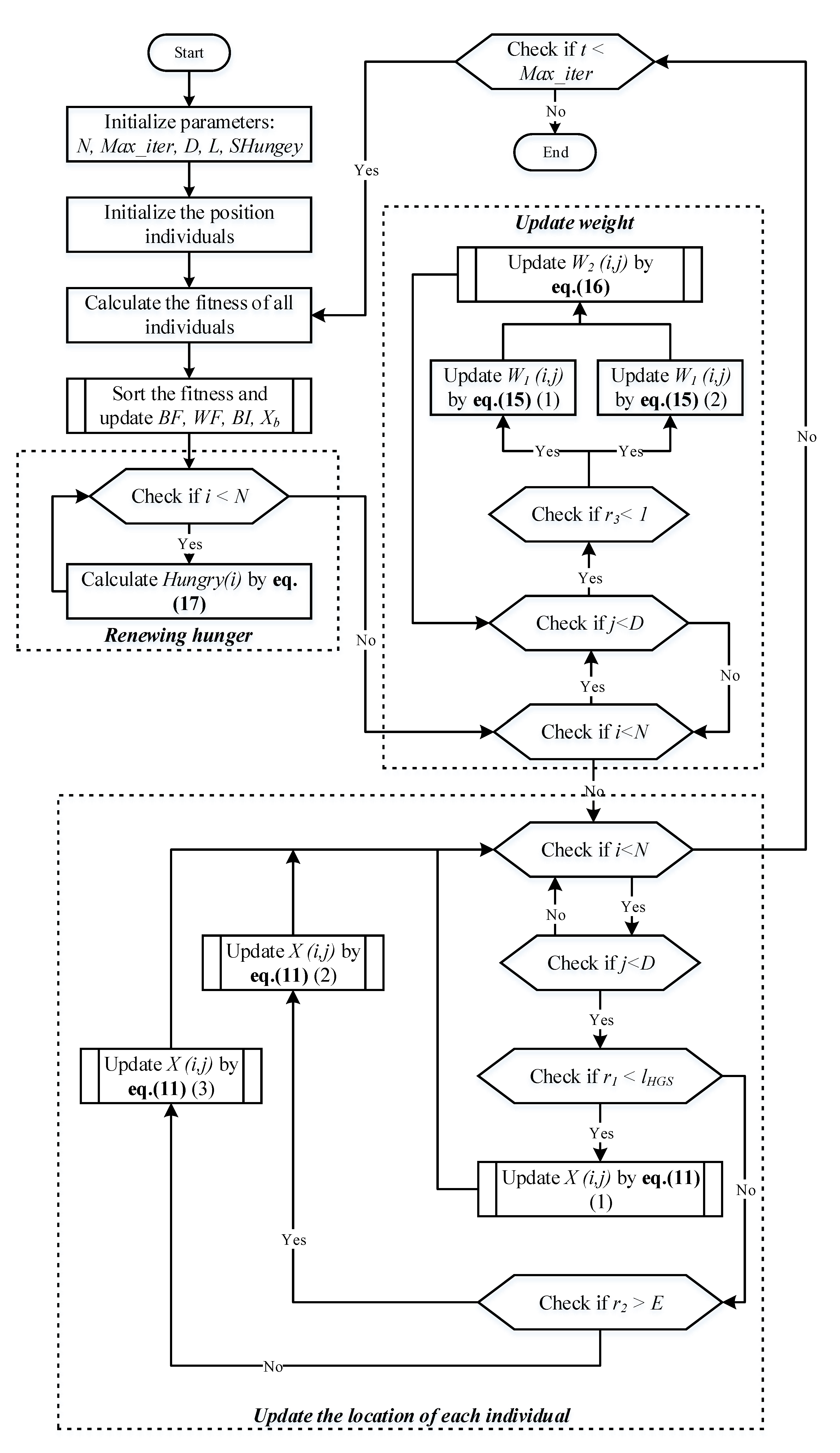
3.4. HGS Pseudo Code and Flowchart

The following pseudo code presents the steps for performing the HGS algorithm:

1:→	Initialize the parameters $N.T.l_{HGS}.D.SHungry$
2:→	Initialize the position of all individuals $X_i\left(i=1,2,\cdots ,N\right)$
3:→	While$\left(t\le T\right)$
4:→	Calculate the fitness of all individuals
5:→	Update $BF.WF.X_b.BI$
6:→	Calculate the $Hungry$ using Equation (17); $W_1$ using Equation (15); $W_2$ using Equation (16);
7:→	For each individual
8:→	Calculate $E$ using Equation (12); update $R$ using Equation (13); update positions using Equation (11)
9:→	End For
10:→	$t=t+1$
11:→	End While
12:→	Return$BF.and{X}_b$

To sum up the previous equations of the HGS algorithm, Figure 1 presents the steps needed to perform the HGS algorithm:

3.5. Problem Formulation

To find the seven unknown parameters of the PEMFC model described in Section 2, it was considered to be an optimization problem with nonlinear constraints. In this problem, the SSD was calculated on the basis of measured and proposed model voltage points. The fitness function was minimized using the HGS algorithm to ensure matching values from both theoretical and actual measurements. The formula describing SSD can be found in [6,7,29,30,31,32,33,34,35,36,38,39,40,42,43,44,45,46,47] and is as follows:

$$SSD={\displaystyle \sum }_{k=1}^n{\left(V_m\left(k\right)-V_e\left(k\right)\right)}^2$$

(20)

Meanwhile, the fitness function $FF$ has the following formula:

$$FF=Minimize\left(SSD\right)$$

(21)

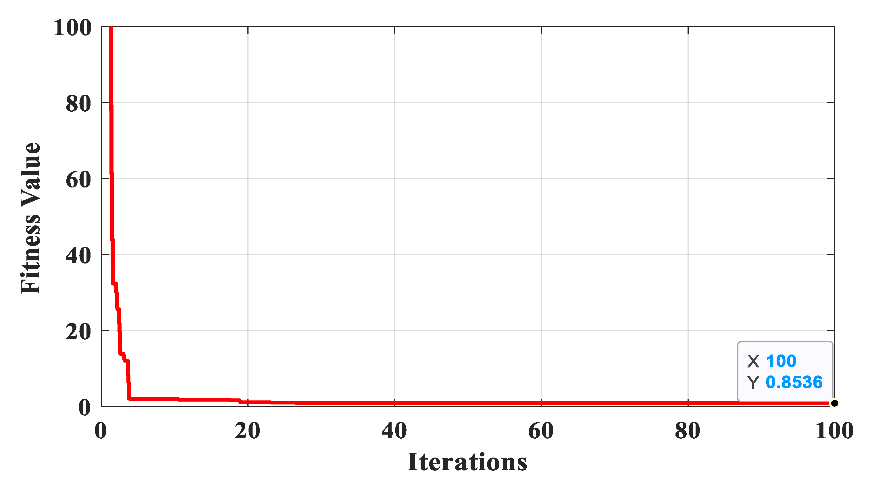
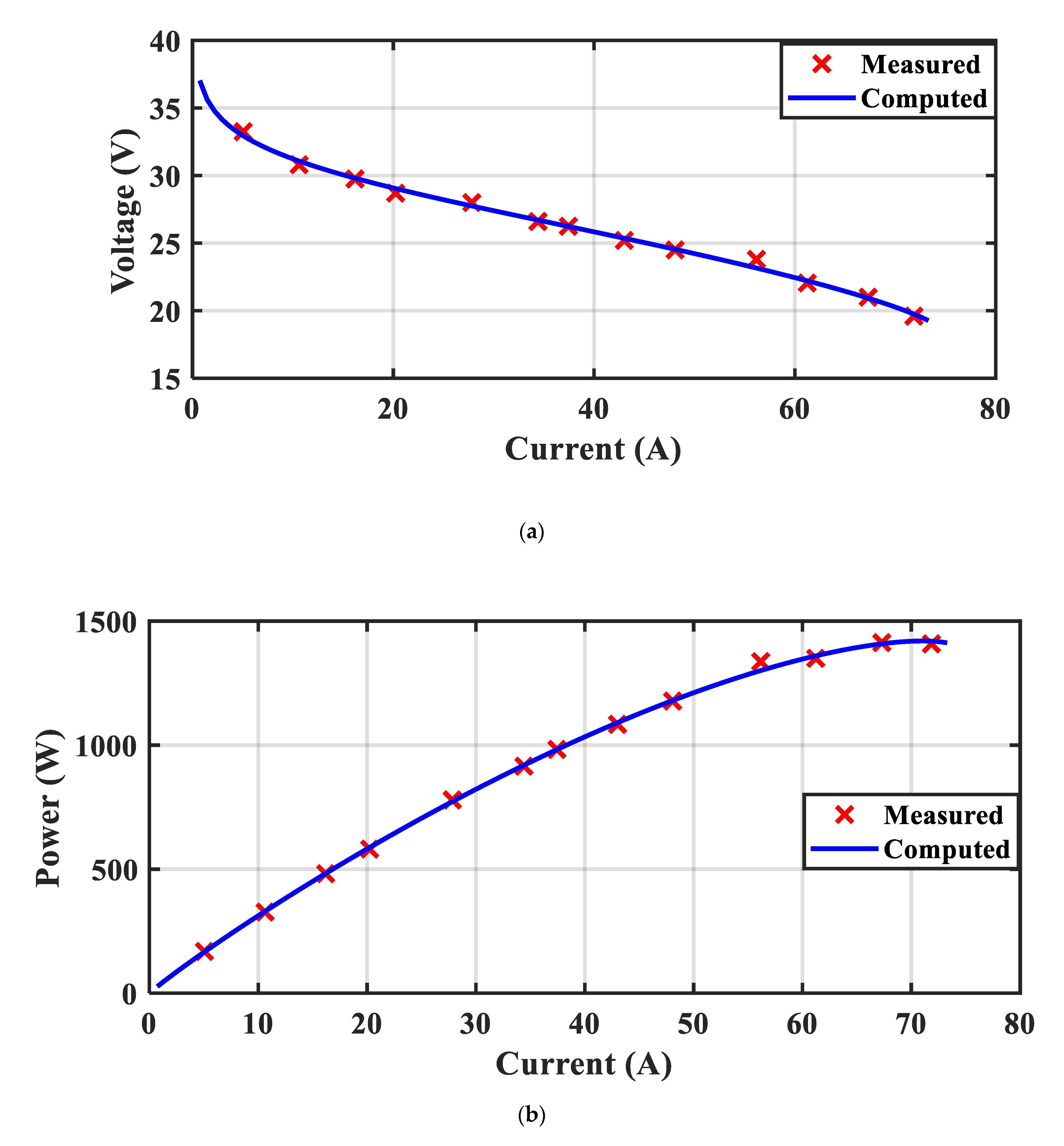
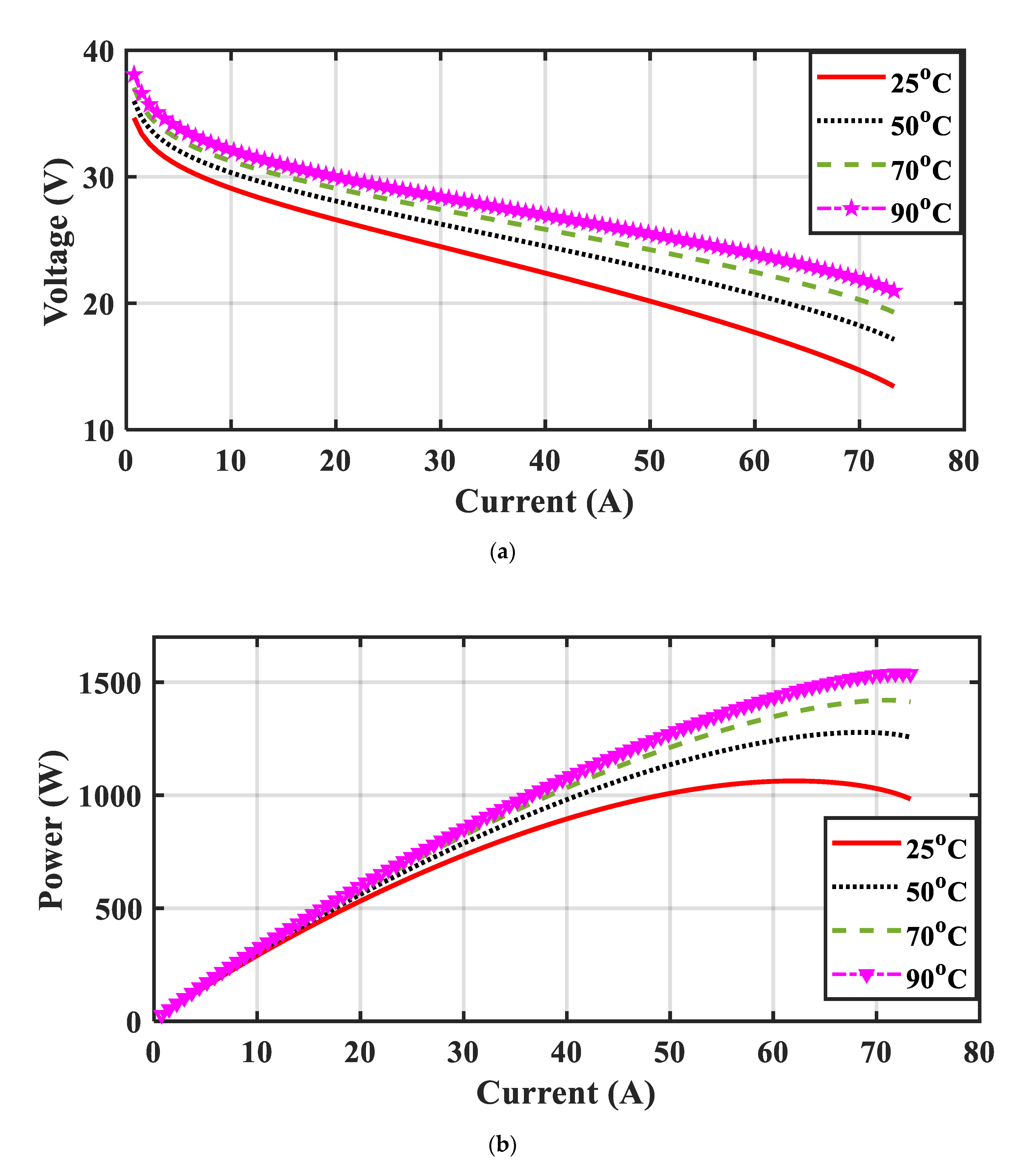
4. Simulation Results

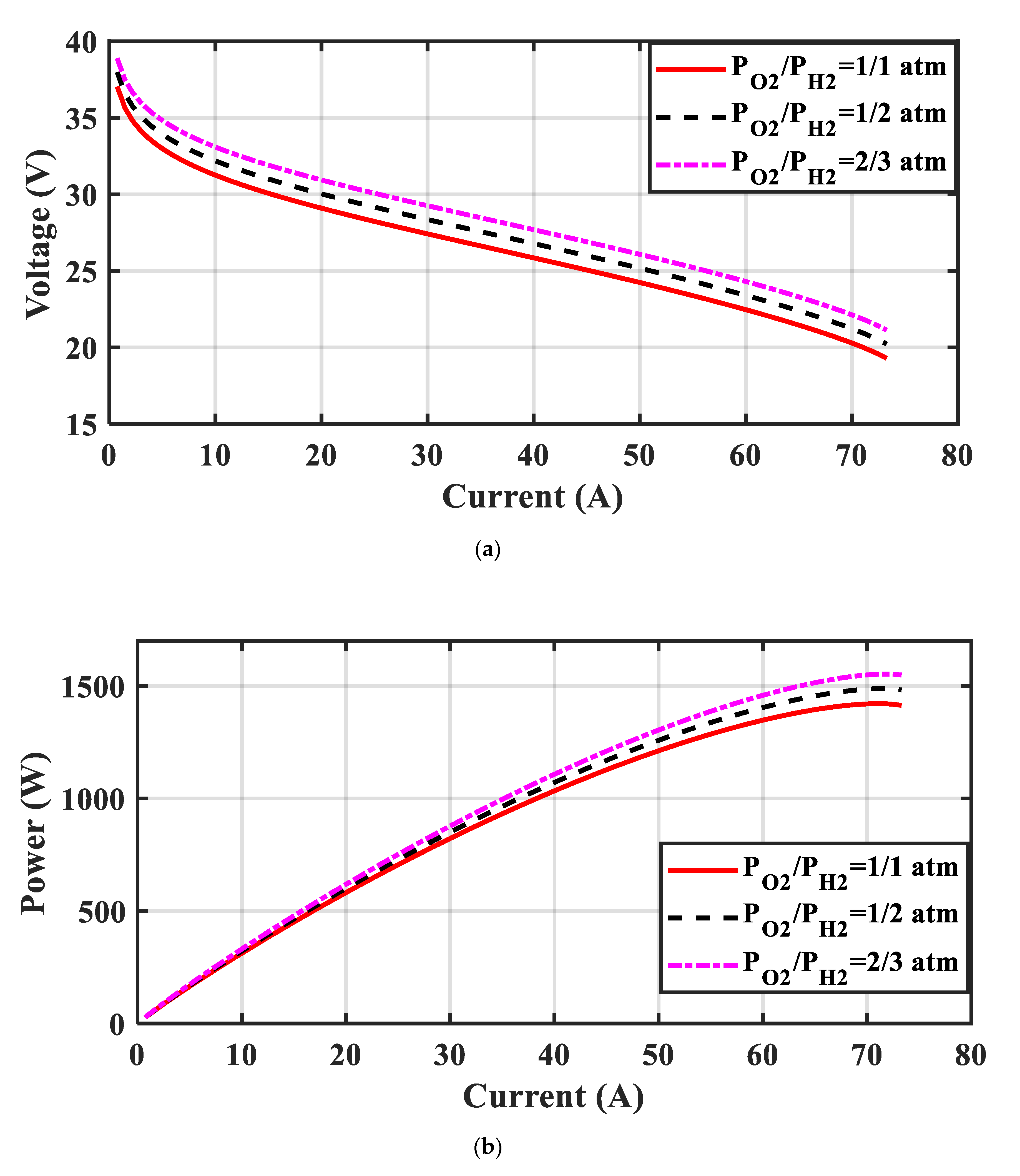
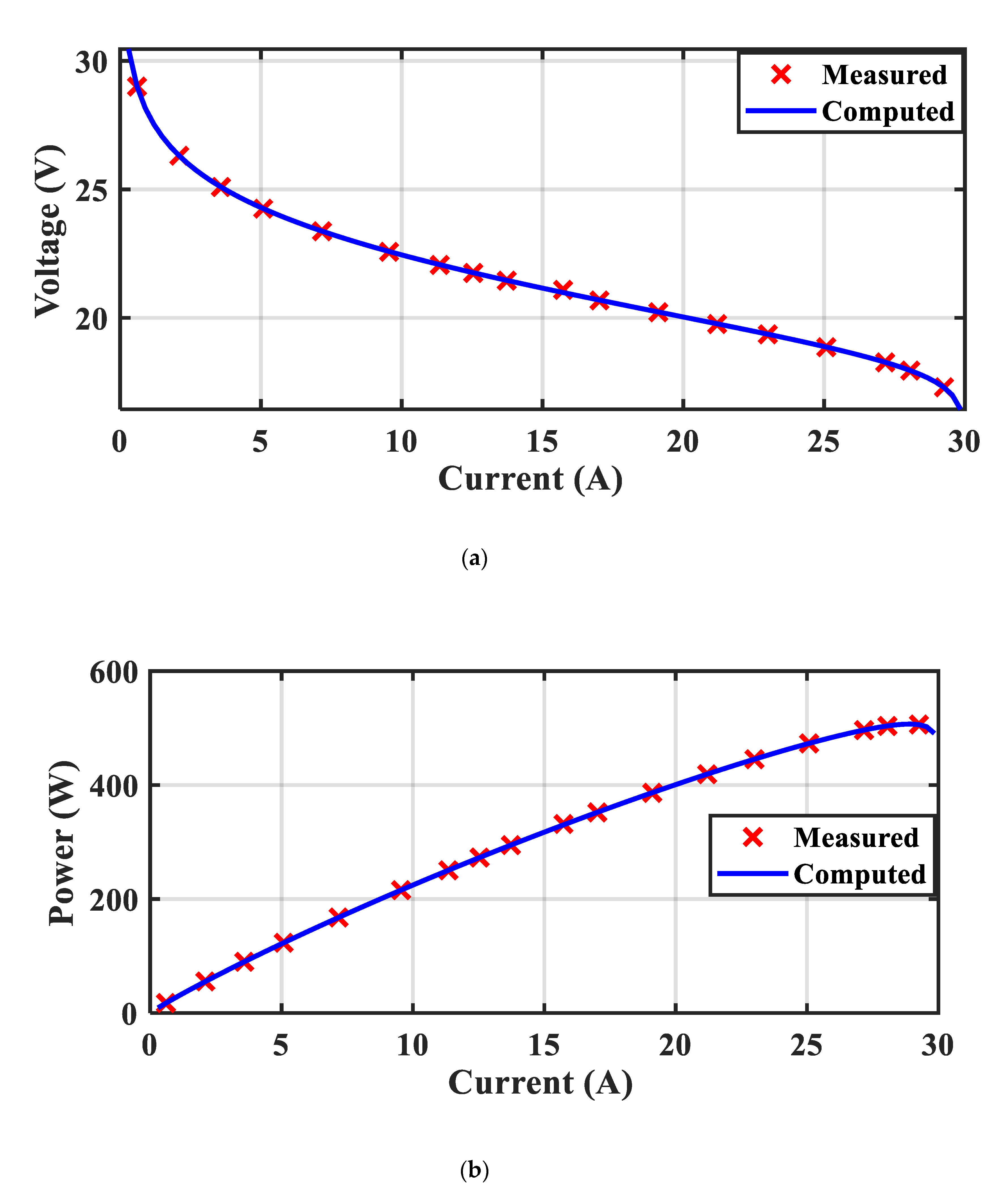
In this study, the proposed HGS algorithm was applied directly to obtain the unknown parameters of the PEMFC model. To this end, the PEMFC model was considered nonlinear model, possessing a nonlinear nature due the impact of temperature and hydrogen and oxygen pressure. The HGS algorithm was implemented to minimize the objective function, yielding accurate parameters for the fuel cell model. To achieve this end, some commercial PEMFCs were tested, including Ballard Mark V, BCS 500 W, and Nedstack PS6. The detailed datasheets for these fuel cells provided in the vast literature available, while the search space limits for the unknown parameters are provided in [7]. The optimization problem under study was considered as an offline optimization problem, which entails the computational effort not being determinant. The simulations were carried out using the MATLAB program, version R2019a. The PC comprised an Intel(R) Core ™ i7 CPU, 2.6 GHz operating Microsoft Windows 10. The PEM fuel cell model and the proposed HGS algorithm codes were built using the MATLAB environment. The optimal settings of the HGS algorithm involved 50 agents and 100 iterations. Actually, these settings were selected by the designer in order to obtain precise results. To check the robustness of the proposed HGS algorithm, 100 independent simulation runs were performed, and some statistical data were obtained, such as the best value, worst value, and standard deviation (SD). The following subsections provide a detailed analysis of this PEMFC modeling.

4.1. Ballard Mark V

The Ballard V 5 kW PEMFC possesses thirty-five cells, which are connected in series. The maximum current of this fuel cell is 70 A. The proposed HGS algorithm was implemented to minimize the objective function in order to accurately obtain the PEM fuel cell model parameters. Several runs were performed, and the best values were chosen. The convergence curve of objective function is illustrated in Figure 2. Notably, this convergence curve is very smooth, with no fluctuations, and it reaches its final value in an expeditious way.

Table 1. Optimal parameters of the Ballard PEMFC model.

Parameter	HGSA	NNA [7]	GOA [44]
${\xi }_1$	−0.991	−0.979	−0.853
${\xi }_2\times {10}^{-3}$	3.70	3.694	3.417
${\xi }_3\times {10}^{-5}$	9.1	9.087	9.8
${\xi }_4\times {10}^{-5}$	−16.35	−16.28	−15.95
$\lambda$	22.87	23	22.84
$R_c\left(m\mathsf{\Omega }\right)$	0.1	0.1	0.1
$\beta$	0.0135	0.0136	0.0136
Best value	0.85360	0.85361	0.871
Worst value	0.861	0.8706	0.909
SD	4.6 × 10−4	0.0085	0.011

reports the optimal values of the unknown parameters of the Ballard PEMFC model using the proposed HGS algorithm in comparison with other models using other optimization algorithms. The statistical analysis presented in Table 1. It can be observed that the HGS-based PEMFC model results in a lower fitness value and SD, which demonstrates its superiority with respect to other approaches reported in the literature. This leads to an accurate model of the PEMFC. The current–voltage (I–V) and current–power (I–P) curves of this fuel cell model are shown in Figure 3a,b, respectively. The HGS-based fuel cell model results are compared with their experimental results in Figure 3. It is worth mentioning here that the proposed PEM fuel cell model is very close to the experimental model, and it achieves a very small error that lies within an acceptable range. Moreover, the simulation of the HGS-based fuel cell model was performed under different temperature and pressure conditions. Figure 4a,b depicts the I–V and I–P curves of this fuel cell model under various temperature conditions (25, 50, 70 and $90{}^{\mathrm{o}}\mathrm{C}$), while maintaining the oxygen and hydrogen pressures constant at one atmospheric pressure. It can be observed that as the fuel cell temperature increases, the PEMFC voltage and power increases. Furthermore, Figure 5a,b show the I–V and I–P curves of the fuel cell model under various pressure conditions while maintaining the fuel cell temperature constant at $70{}^{\mathrm{o}}\mathrm{C}$. It can be noted that as the partial pressure of oxygen and/or hydrogen increases, the voltage and power of the fuel cell increase. Therefore, these pressures can be carefully adjusted to achieve specific output power from the fuel cell under specific environmental conditions.

4.2. BCS Fuel Cell

The BCS 500 W fuel cell has thirty-two cells, which are connected in series. This fuel cell is fabricated using BCS technology. The maximum current of the fuel cell is 30 A. The proposed HGS algorithm was implemented to minimize the objective function in order to accurately obtain the PEMFC model parameters. Several runs were performed and the best values were chosen. The convergence curve of objective function is illustrated in Figure 6. It can be observed here that the convergence curve is smooth, and it quickly reaches the final value.

Table 2. Optimal parameters of the BCS PEMFC model.

Parameter	HGSA	NNA [7]K	SFLA [40]	ICA [40]	FOA [40]	SSO [39]
${\xi }_1$	−1.11	−1.059	−0.965	−0.908	−0.992	−0.853
${\xi }_2\times {10}^{-3}$	3.753	3.743	3.081	2.479	2.621	4.811
${\xi }_3\times {10}^{-5}$	9.71	9.69	7.223	4.458	3.746	9.433
${\xi }_4\times {10}^{-5}$	−19.35	−19.302	−19.3	−19.31	−19.30	−19.205
$\lambda$	20.97	20.87	20.886	22.66	21.101	23
$R_c\left(m\mathsf{\Omega }\right)$	0.1	0.1	0.1	0.246	0.1	0.349
$\beta$	0.0161	0.0161	0.0161	0.0162	0.01630	0.0158
Best value	0.011692	0.011698	0.011697	0.01185	0.01181	0.0122
Worst value	0.0134	0.01367	0.01169	0.03466	0.03023	0.0152
SD	3.4 × 10−4	$5.641\times {10}^{-4}$	$5.04\times {10}^{-8}$	0.00587	0.0041	$8.71\times {10}^{-4}$

demonstrates the optimal values of the unknown parameters of the BCS fuel cell model using the HGS algorithm in comparison with other models using other optimization algorithms. The statistical analysis is provided in Table 2. It can be noted that the HGS-based PEMFC model leads to lower fitness values and SD. This indicates its great superiority over the other models reported in the literature. This indicates that an accurate model of the PEMFC was obtained. The polarization curves (I–V) and (I–P) of the BCS fuel cell model using the proposed HGS algorithm are shown in Figure 7a,b, respectively. The results for the HGS-based fuel cell model are compared with the experimental results in Figure 7. It is worth mentioning here that the proposed PEMFC model coincides with the experimental model.

Furthermore, the simulation results of the HGS-based fuel cell model were obtained under different temperature and pressure conditions. Figure 8a,b provide the I–V and I–P curves of this fuel cell model under various temperature conditions (30, 50, and ${70}^{\mathrm{o}}\mathrm{C}$), while maintaining the oxygen and hydrogen pressures at one atmospheric pressure. It can be observed that as the fuel cell temperature increases, the voltage and power of the PEMFC increase. Furthermore, Figure 9a,b show the I–V and I–P curves of the fuel cell model under various pressure conditions while maintaining the temperature of the fuel cell temperature at $60{}^{\mathrm{o}}\mathrm{C}$. It can be noted that as the partial pressure of oxygen and/or hydrogen increases, the voltage and power of the fuel cell increase. Therefore, these pressures can be carefully adjusted to achieve specific output power from the fuel cell under specific environmental conditions.

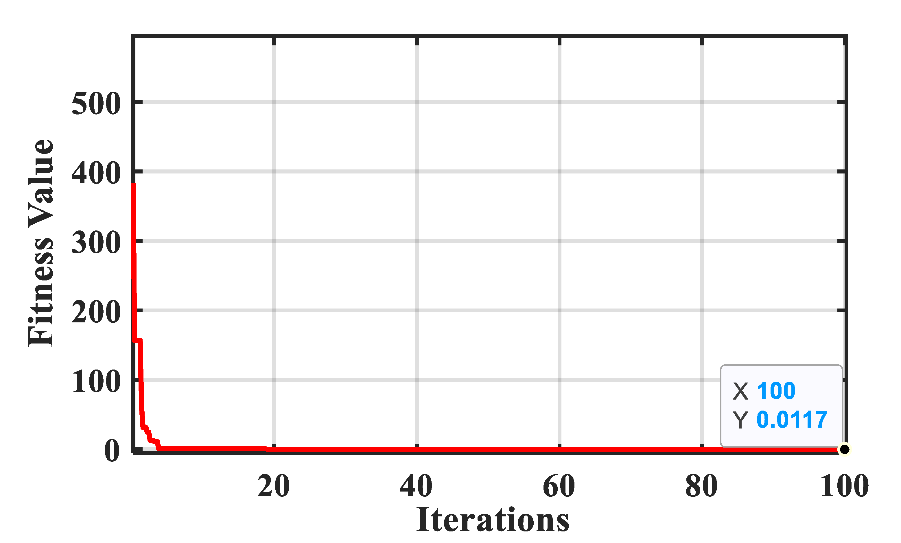
4.3. Robustness of the Proposed HGS Algorithm

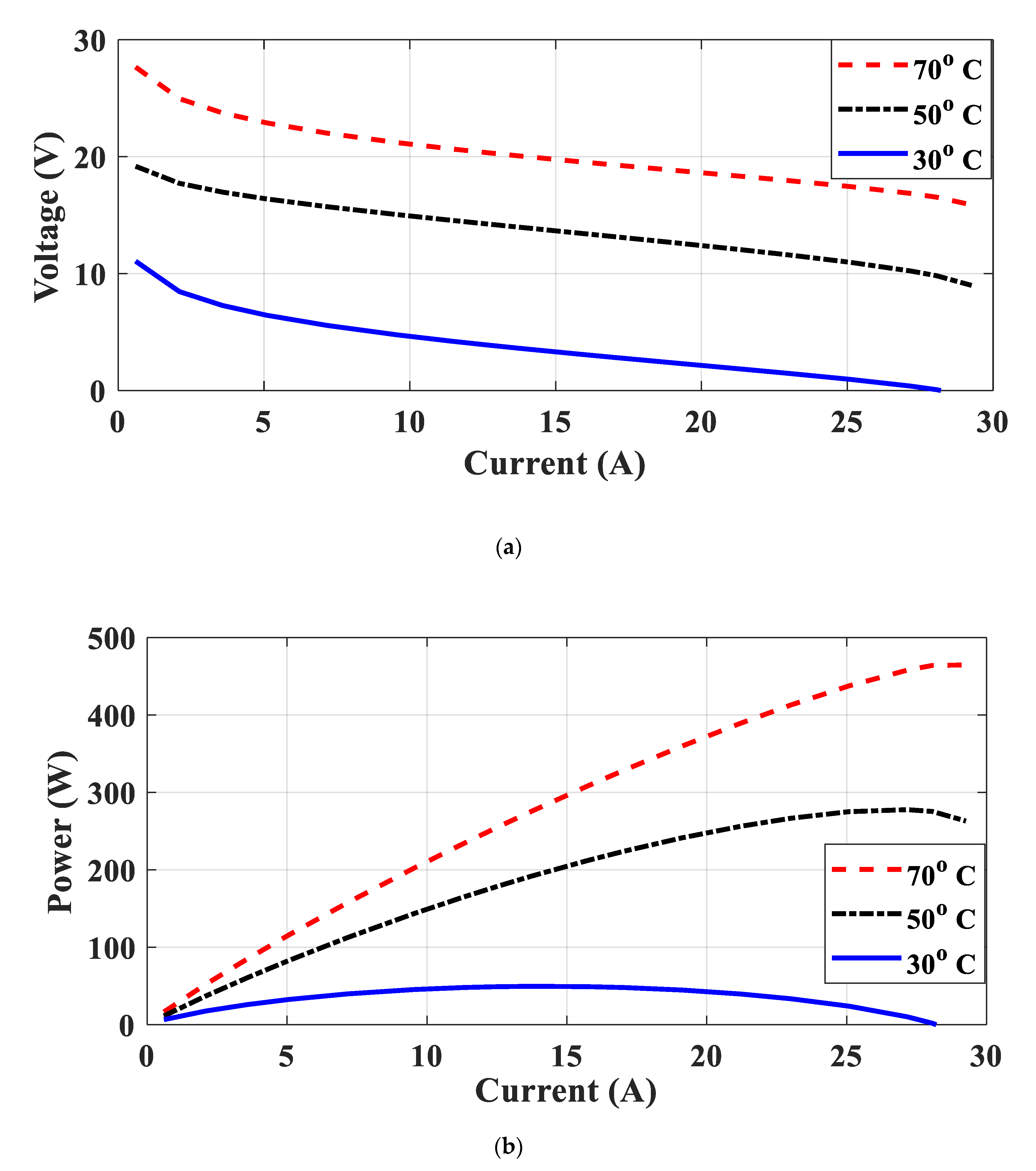
To check the robustness of the proposed HGS algorithm, the hypothesis t-test was implemented in the Ballard PEMFC model. The hypothesis test is a procedure used to ensure that the characteristics of the population are correct. The goal test checks the statistical evidence for accepting the null hypothesis. To this end, 20 independent runs were carried out on the HGS-based PEMFC model, and the fitness values of each of these runs were recorded and used in the t-test, which was performed using the MATLAB environment. The test employed a 5% level of significance. The h-value and P-value were recorded as 0 and 1, respectively. The value of the test statistics was 0. The degree of freedom of these test records was 19 and the standard deviation was 4.9 × 10⁻⁶. These statistical measurements indicate the high robustness of the proposed HGS algorithm-based PEMFC model.

4.4. Discussion

The proposed HGS algorithm was effectively implemented in order to obtain the unknown parameters of the PEMFC model. As demonstrated in the previous subsections, the proposed algorithm provided the lowest fitness value among the results obtained from other algorithms. This demonstrates its superiority for solving the optimization problem under study. This high performance of the proposed algorithm comes from its appropriate design, which depends on the experience of the designer in finding its optimal settings. Moreover, the proposed algorithm possesses a high convergence speed, with a minimal number of parameters needing to be tuned. This has encouraged many researchers to use it to solve many engineering problems. There is a lack of studies focusing on finding suitable environments in which to operate and store hydrogen pipes, where safety is dependent on certain temperature and pressure requirements.

5. Conclusions

This paper presented a novel application of the HGS algorithm to efficiently identify the PEMFC model parameters. The PEMFC model can affect the simulation results of fuel cells and their analyses, having dramatic implications in many applications, such as distributed generation, microgrids, and smart grid systems. The fitness function is based on the sum of square error between the identified voltage model and the experimental voltage. The design variables of the model comprise seven unknown model parameters. The proposed HGS algorithm is applied to minimize the fitness function, and yields the design variables under varying constraints. In fact, this optimization problem was built in response to the shortage of PEMFC data provided by the manufacturers. The simulation results of the HGS-based model demonstrated its accuracy in comparison with the experimental results. Moreover, the simulation results demonstrated the capability and flexibility of the model for studying fuel cells under different environmental conditions (i.e., temperature and partial pressure of oxygen and/hydrogen). The results obtained using HGS outperformed those obtained with other optimizers, which was a result of the proper design of the HGS algorithm. The robustness of the HGS algorithm was successfully tested on the basis of several statistical analyses and the parametric t-test, achieving superior values. With the proposed HGS-based fuel cell model, accurate modeling of the fuel cell can be performed. Moreover, the proposed algorithm can be applied to solve other power engineering problem such as those in renewable energy and smart grid systems.

References

1. Yakout, A.H.; Hasanien, H.M.; Kotb, H. Proton Exchange Membrane Fuel Cell Steady State Modeling Using Marine Predator Algorithm Optimizer. Ain Shams Eng. J. 2021. [Google Scholar] [CrossRef]
2. Hasanien, H.; Matar, M. A Fuzzy Logic Controller for Autonomous Operation of a Voltage Source Converter-Based Distributed Generation System. IEEE Trans. Smart Grid 2015, 6, 158–165. [Google Scholar] [CrossRef]
3. Liu, J.; Xu, Z.; Wu, J.; Liu, K.; Guan, X. Optimal planning of distributed hydrogen-based multi-energy systems. Appl. Energy 2020, 281, 116107. [Google Scholar] [CrossRef]
4. El-Hay, E.; El-Hameed, M.A.; El-Fergany, A. Optimized Parameters of SOFC for steady state and transient simulations using interior search algorithm. Energy 2018, 166, 451–461. [Google Scholar] [CrossRef]
5. Nejad, H.C.; Farshad, M.; Gholamalizadeh, E.; Askarian, B.; Akbarimajd, A. A novel intelligent-based method to control the output voltage of Proton Exchange Membrane Fuel Cell. Energy Convers. Manag. 2019, 185, 455–464. [Google Scholar] [CrossRef]
6. El-Hay, E.; El-Hameed, M.; El-Fergany, A. Steady-state and dynamic models of solid oxide fuel cells based on Satin Bowerbird Optimizer. Int. J. Hydrogen Energy 2018, 43, 14751–14761. [Google Scholar] [CrossRef]
7. Fawzi, M.; El-Fergany, A.A.; Hasanien, H.M. Effective methodology based on neural network optimizer for extracting model parameters of PEM fuel cells. Int. J. Energy Res. 2019, 43, 8136–8147. [Google Scholar] [CrossRef]
8. El-Fergany, A.A.; Hasanien, H.M.; Agwa, A.M. Semi-empirical PEM fuel cells model using whale optimization algorithm. Energy Convers. Manag. 2019, 201, 112197. [Google Scholar] [CrossRef]
9. Gong, W.; Yan, X.; Hu, C.; Wang, L.; Gao, L. Fast and accurate parameter extraction for different types of fuel cells with decomposition and nature-inspired optimization method. Energy Convers. Manag. 2018, 174, 913–921. [Google Scholar] [CrossRef]
10. Agwa, A.M.; El-Fergany, A.A.; Sarhan, G.M. Steady-State Modeling of Fuel Cells Based on Atom Search Optimizer. Energies 2019, 12, 1884. [Google Scholar] [CrossRef] [Green Version]
11. Sun, L.; Jin, Y.; Pan, L.; Shen, J.; Lee, K.Y. Efficiency analysis and control of a grid-connected PEM fuel cell in distributed generation. Energy Convers. Manag. 2019, 195, 587–596. [Google Scholar] [CrossRef]
12. Bizon, N.; Mazare, A.-G.; Ionescu, L.-M.; Enescu, F.M. Optimization of the proton exchange membrane fuel cell hybrid power system for residential buildings. Energy Convers. Manag. 2018, 163, 22–37. [Google Scholar] [CrossRef]
13. El-Hay, E.A.; El-Hameed, M.A.; El-Fergany, A.A. Performance enhancement of autonomous system comprising proton exchange membrane fuel cells and switched reluctance motor. Energy 2018, 163, 699–711. [Google Scholar] [CrossRef]
14. Zhang, G.; Xie, B.; Bao, Z.; Niu, Z.; Jiao, K. Multi-phase simulation of proton exchange membrane fuel cell with 3D fine mesh flow field. Int. J. Energy Res. 2018, 42, 4697–4709. [Google Scholar] [CrossRef]
15. Budak, Y.; Devrim, Y. Investigation of micro-combined heat and power application of PEM fuel cell systems. Energy Convers. Manag. 2018, 160, 486–494. [Google Scholar] [CrossRef]
16. Karanfil, G. Importance and applications of DOE/optimization methods in PEM fuel cells: A review. Int. J. Energy Res. 2019, 44, 4–25. [Google Scholar] [CrossRef]
17. Guo, C.; Lu, J.; Tian, Z.; Guo, W.; Darvishan, A. Optimization of critical parameters of PEM fuel cell using TLBO-DE based on Elman neural network. Energy Convers. Manag. 2019, 183, 149–158. [Google Scholar] [CrossRef]
18. Bankupalli, P.T.; Ghosh, S.; Kumar, L.; Samanta, S.; Dixit, T.V. A non-iterative approach for maximum power extraction from PEM fuel cell using resistance estimation. Energy Convers. Manag. 2019, 187, 565–577. [Google Scholar] [CrossRef]
19. Massonnat, P.; Gao, F.; Roche, R.; Paire, D.; Bouquain, D.; Miraoui, A. Multiphysical, multidimensional real-time PEM fuel cell modeling for embedded applications. Energy Convers. Manag. 2014, 88, 554–564. [Google Scholar] [CrossRef]
20. Ritzberger, D.; Striednig, M.; Simon, C.; Hametner, C.; Jakubek, S. Online estimation of the electrochemical impedance of polymer electrolyte membrane fuel cells using broad-band current excitation. J. Power Sources 2018, 405, 150–161. [Google Scholar] [CrossRef]
21. Taleb, M.A.; Béthoux, O.; Godoy, E. Identification of a PEMFC fractional order model. Int. J. Hydrogen Energy 2017, 42, 1499–1509. [Google Scholar] [CrossRef]
22. Murschenhofer, D.; Kuzdas, D.; Braun, S.; Jakubek, S. A real-time capable quasi-2D proton exchange membrane fuel cell model. Energy Convers. Manag. 2018, 162, 159–175. [Google Scholar] [CrossRef]
23. Geem, Z.W.; Noh, J.-S. Parameter Estimation for a Proton Exchange Membrane Fuel Cell Model Using GRG Technique. Fuel Cells 2016, 16, 640–645. [Google Scholar] [CrossRef]
24. Jiang, Y.; Yang, Z.; Jiao, K.; Du, Q. Sensitivity analysis of uncertain parameters based on an improved proton exchange membrane fuel cell analytical model. Energy Convers. Manag. 2018, 164, 639–654. [Google Scholar] [CrossRef]
25. Aouali, F.; Becherif, M.; Ramadan, H.; Emziane, M.; Khellaf, A.; Mohammedi, K. Analytical modelling and experimental validation of proton exchange membrane electrolyser for hydrogen production. Int. J. Hydrogen Energy 2017, 42, 1366–1374. [Google Scholar] [CrossRef]
26. Chavan, S.; Talange, D.B. System identification black box approach for modeling performance of PEM fuel cell. J. Energy Storage 2018, 18, 327–332. [Google Scholar] [CrossRef]
27. Zhang, L.; Wang, N. An adaptive RNA genetic algorithm for modeling of proton exchange membrane fuel cells. Int. J. Hydrogen Energy 2012, 38, 219–228. [Google Scholar] [CrossRef]
28. Cao, Y.; Li, Y.; Zhang, G.; Jermsittiparsert, K.; Razmjooy, N. Experimental modeling of PEM fuel cells using a new improved seagull optimization algorithm. Energy Rep. 2019, 5, 1616–1625. [Google Scholar] [CrossRef]
29. Chen, Y.; Wang, N. Cuckoo search algorithm with explosion operator for modeling proton exchange membrane fuel cells. Int. J. Hydrogen Energy 2019, 44, 3075–3087. [Google Scholar] [CrossRef]
30. Sun, Z.; Wang, N.; Bi, Y.; Srinivasan, D. Parameter identification of PEMFC model based on hybrid adaptive differential evolution algorithm. Energy 2015, 90, 1334–1341. [Google Scholar] [CrossRef]
31. Gong, W.; Cai, Z. Parameter optimization of PEMFC model with improved multi-strategy adaptive differential evolution. Eng. Appl. Artif. Intell. 2014, 27, 28–40. [Google Scholar] [CrossRef]
32. Gong, W.; Yan, X.; Liu, X.; Cai, Z. Parameter extraction of different fuel cell models with transferred adaptive differential evolution. Energy 2015, 86, 139–151. [Google Scholar] [CrossRef]
33. Ali, M.; El-Hameed, M.; Farahat, M. Effective parameters’ identification for polymer electrolyte membrane fuel cell models using grey wolf optimizer. Renew. Energy 2017, 111, 455–462. [Google Scholar] [CrossRef]
34. Askarzadeh, A.; Coelho, L.D.S. A backtracking search algorithm combined with Burger's chaotic map for parameter estimation of PEMFC electrochemical model. Int. J. Hydrogen Energy 2014, 39, 11165–11174. [Google Scholar] [CrossRef]
35. Zhang, W.; Wang, N.; Yang, S. Hybrid artificial bee colony algorithm for parameter estimation of proton exchange membrane fuel cell. Int. J. Hydrogen Energy 2013, 38, 5796–5806. [Google Scholar] [CrossRef]
36. Xu, S.; Wang, Y.; Wang, Z. Parameter estimation of proton exchange membrane fuel cells using eagle strategy based on JAYA algorithm and Nelder-Mead simplex method. Energy 2019, 173, 457–467. [Google Scholar] [CrossRef]
37. Duan, B.; Cao, Q.; Afshar, N. Optimal parameter identification for the proton exchange membrane fuel cell using Satin Bowerbird optimizer. Int. J. Energy Res. 2019. [Google Scholar] [CrossRef]
38. Rao, Y.; Shao, Z.; Ahangarnejad, A.H.; Gholamalizadeh, E.; Sobhani, B. Shark Smell Optimizer applied to identify the optimal parameters of the proton exchange membrane fuel cell model. Energy Convers. Manag. 2019, 182, 1–8. [Google Scholar] [CrossRef]
39. El-Fergany, A. Extracting optimal parameters of PEM fuel cells using Salp Swarm Optimizer. Renew. Energy 2018, 119, 641–648. [Google Scholar] [CrossRef]
40. Kandidayeni, M.; Macias, A.; Khalatbarisoltani, A.; Boulon, L.; Kelouwani, S. Benchmark of proton exchange membrane fuel cell parameters extraction with metaheuristic optimization algorithms. Energy 2019, 183, 912–925. [Google Scholar] [CrossRef]
41. Askarzadeh, A.; Rezazadeh, A. An Innovative Global Harmony Search Algorithm for Parameter Identification of a PEM Fuel Cell Model. IEEE Trans. Power Electron. 2011, 59, 3473–3480. [Google Scholar] [CrossRef]
42. Fathy, A.; Elaziz, M.A.; Alharbi, A.G. A novel approach based on hybrid vortex search algorithm and differential evolution for identifying the optimal parameters of PEM fuel cell. Renew. Energy 2020, 146, 1833–1845. [Google Scholar] [CrossRef]
43. Priya, K.; Rajasekar, N. Application of flower pollination algorithm for enhanced proton exchange membrane fuel cell modelling. Int. J. Hydrogen Energy 2019, 44, 18438–18449. [Google Scholar] [CrossRef]
44. El-Fergany, A. Electrical characterisation of proton exchange membrane fuel cells stack using grasshopper optimiser. IET Renew. Power Gener. 2017, 12, 9–17. [Google Scholar] [CrossRef]
45. Askarzadeh, A.; Rezazadeh, A. Optimization of PEMFC model parameters with a modified particle swarm optimization. Int. J. Energy Res. 2010, 35, 1258–1265. [Google Scholar] [CrossRef]
46. Fathy, A.; Rezk, H. Multi-verse optimizer for identifying the optimal parameters of PEMFC model. Energy 2018, 143, 634–644. [Google Scholar] [CrossRef]
47. Niu, Q.; Zhang, H.; Li, K. An improved TLBO with elite strategy for parameters identification of PEM fuel cell and solar cell models. Int. J. Hydrogen Energy 2014, 39, 3837–3854. [Google Scholar] [CrossRef]
48. Wolpert, D.; Macready, W. Coevolutionary Free Lunches. IEEE Trans. Evol. Comput. 2005, 9, 721–735. [Google Scholar] [CrossRef]
49. Yang, Y.; Chen, H.; Heidari, A.A.; Gandomi, A.H. Hunger games search: Visions, conception, implementation, deep analysis, perspectives, and towards performance shifts. Expert Syst. Appl. 2021, 177, 114864. [Google Scholar] [CrossRef]
50. Gurung, A.; Oh, S.-E. The Performance of Serially and Parallelly Connected Microbial Fuel Cells. Energy Sources, Part A: Recover. Util. Environ. Eff. 2012, 34, 1591–1598. [Google Scholar] [CrossRef]
51. Mann, R.F.; Amphlett, J.C.; Hooper, M.A.; Jensen, H.M.; Peppley, B.A.; Roberge, P.R. Development and application of a generalised steady-state electrochemical model for a PEM fuel cell. J. Power Sources 2000, 86, 173–180. [Google Scholar] [CrossRef]
Figure 1. Flowchart of the HGS algorithm.
Energies 14 05022 g001
Figure 2. Convergence of the objective function of the Ballard PEMFC model.
Energies 14 05022 g002
Figure 3. Polarization curves of Ballard fuel cell using the HGS algorithm. (a) I–V curves. (b) I–P curves.
Energies 14 05022 g003
Figure 4. Polarization curves of Ballard fuel cell using the HGS algorithm under various temperature conditions at constant pressure. (a) I–V curves. (b) I–P curves.
Energies 14 05022 g004
Figure 5. Polarization curves of Ballard fuel cell using the HGS algorithm under various pressure conditions with constant temperature. (a) I–V curves. (b) I–P curves.
Energies 14 05022 g005
Figure 6. Convergence of the objective function of the BCS PEMFC model.
Energies 14 05022 g006
Figure 7. Polarization curves of BCS fuel cell using the HGS algorithm. (a) I–V curves. (b) I–P curves.
Energies 14 05022 g007
Figure 8. Polarization curves of BCS fuel cell using the HGS algorithm under various temperature conditions at constant pressure. (a) I–V curves. (b) I–P curves.
Energies 14 05022 g008
Figure 9. Polarization curves of Ballard fuel cells using the HGS algorithm under various pressure conditions at constant temperatures. (a) I–V curves. (b) I–P curves.
Energies 14 05022 g009