Comparison of the Efficiency and Load Power in Periodic Wireless Power Transfer Systems with Circular and Square Planar Coils

Abstract

In the article, a wireless charging system with the use of periodically arranged planar coils is presented. The efficiency of two wireless power transfer (WPT) systems with different types of inductors, i.e., circular and square planar coils is compared, and two models are proposed: analytical and numerical. With the appropriate selection of a load resistance, it is possible to obtain either the maximum efficiency or the maximum power of a receiver. Therefore, the system is analyzed at two optimum modes of operation: with the maximum possible efficiency and with the highest power transmitted to the load. The analysis of many variants of the proposed wireless power transfer solution was performed. The aim was to check the influence of the geometry of the coils and their type (circular or square) on the efficiency of the system. Changes in the number of turns, the distance between the coils (transmit and receive) as well as frequency are also taken into account. The results obtained from analytical and numerical analysis were consistent; thus, the correctness of the adopted circuit and numerical model (with periodic boundary conditions) was confirmed. The proposed circuit model and the presented numerical approach allow for a quick estimate of the electrical parameters of the wireless power transmission system. The proposed system can be used to charge many receivers, e.g., electrical cars on a parking or several electronic devices. Based on the results, it was found that the square coils provide lower load power and efficiency than compared to circular coils in the entire frequency range and regardless of the analyzed geometry variants. The results and discussion of the multivariate analysis allow for a better understanding of the influence of the coil geometry on the charging effectiveness. They can also be valuable knowledge when designing this type of system.

1. Introduction

Power in the form of electricity generated in power plants is expensive, and the overall efficiency of the transmission from plants to end users is low (about 30%), in particular, due to energy losses in parasitic resistances. The power plant itself needs many resources to produce electricity and has many troubles related with environmental issues (e.g., pollution). Additionally, insufficient reactive power compensation, voltage asymmetry and current distortion reduce the efficiency and quality of electricity transferred to consumers [1]. Indicated problems were one of many, which have resulted in alternate solutions connected with power transmission and distribution. The other problems include cables and wires for supplying electrical devices, e.g., at home, workplace and school, since these are lossy elements that are prone to failure and inconvenient to install. Furthermore, devices using batteries can be disturbed and may stop working during battery replacement.

Considering the above, the high-efficiency wireless charging system would be beneficial in both economic and even social approach. Many entities are trying to explore the use of electric vehicles in order to reduce fuel and energy consumption [2,3]. Moreover, the wireless power transfer (WPT) system could result in huge benefits in the medical field in terms of charging or supplying medical devices (e.g., pacemaker and endoscopy) [4,5]. The focus of researchers working on WPT is to develop and research wireless powering equipment for different industries, e.g., medical, factory and private customer.

Wireless power transmission (WPT) has become one of the most important research focuses in this century. Portability is the main motivation for WPT as the number of portable devices is enormously increasing, and wired chargers will limit their portability. Several review works [6,7,8] described the WPT theory and its applications. Still, developments in the resonant coupled system [9,10,11,12], in the influence of couplings and frequency on efficiency and in human exhibition aspects [13,14] have not been widely considered.

The near-field inductive power transfer (IPT) [15,16] has gained popularity for charging mobile consumer devices. The IPT system can effectively transmit power from a source to the device by using the rule of electromagnetic induction. The advantage of this system is the lack of radiation. Inductive devices (e.g., charging pad for cell phone) work according to the same principles.

After the first experiment of the glowing bulb by using resonant coils conducted by MIT (Massachusetts Institute of Technology, Cambridge, MA, USA) in 2007, progress in resonant coupled system has occurred [17]. In 2008, Intel studied the resonant coupled by using surface coils, which are simpler to montage into mobile devices than the helix coils [18]. In [19], a progressive contactless solution for synchronous powering relative to a few receiving devices was discussed. The research studies on IPT have indicated that, for practical applications, the frequency range from 20 kHz to 200 MHz has been considered [20]. Generally speaking, the bandwidth of WPT should have been limited to industrial, scientific and medical (ISM) frequencies, e.g., 13.56 MHz [6]. However, these frequencies are higher than 6.78 MHz, which will cause additional skin and proximity effect losses in copper conductors wider than 0.05 mm (based on a round wire skin depth). Therefore, IPT systems were also designed to operate at lower frequencies, such as wireless electric vehicles power supply at 20.15 kHz [2] and charging of implantable medical sensors (from 300 kHz to 10 MHz) [4]. Hence, it can be acceptable to use WPT at the kHz range if the low-power system will not exceed electromagnetic safety limits. An example of such system may be also periodic WPT, proposed in this article, which can efficiently operate below 1 MHz since multi-turn coils with relatively high inductances are used.

In opposition to the traditional 2-coil approach [21], the 4-coil approach is designed by setting two indirect multi-turn coils between two loop coils. Every loop coil is a mechanism in which impedance matching takes place and works as a non-resonator to exchange energy between circuits and indirect coils [18]. Further works [22,23] related to multi-coil resonant coupling created interest in the 4-coil system due to increased efficiency. The disadvantage of this approach is it requires more space than any other transmission system.

WPT for many receivers using a single source coil has been described and analyzed in [24]. The downside to this approach is that the resonant frequency of the coils is divided when two receivers are close to each other, which reduces the efficiency. In the article [9], the systems of the coils as domino form resonators are presented. The authors of [10] considered linear resonator systems. These systems included several additional resonators located in the middle (between transmitter and receiver). Their task was to support energy transfer in the system. The analysis was conducted for many resonator configurations. However, parallel-series systems containing planar coils are still not completely developed.

The power transfer efficiency falls at any coupling larger or smaller than its critical value. For this reason, it is necessary to use an additional system to maintain the high efficiency. In this approach, the mentioned system must work without movable resonant frequency at coupling length changes. Different approaches (e.g., adjusting resonant parameters) were presented in [25,26,27,28,29,30,31]. Their goal was to transfer power with better efficiency in the resonant coupled system. The influence of axial and angular misalignment of the coils was presented in [32]. This is the main problem in WPT realization for mobile devices.

The power supply of many devices situated close to one another can be realized by using a net of periodically located coils. This approach raises the density of transferred power and also provides possibilities of synchronous energy supply for many devices. Proposed solutions can be used to power either one or multiple independent loads and, in some cases, replace conventional IPT systems. The developed periodic WPT system allows for the simultaneous supply/charging of many low-power receivers, such as mobile devices or sensors repeatedly distributed over hard-to-reach areas.

The article presents the wireless charging system with periodically arranged planar coils. The proposed analysis of the unit cell with periodic boundary conditions does not demand the creation of a 3D model with many coils [33]. This model has many degrees of freedom. The simplified model of equivalent circuit is an alternative for large matrix formulations [9,10,34]. The main goal of this work is to present and analyze WPT systems, including circular or square coils. The proposed system may be used for analyzing power transfer conditions.

Two analysis approaches have been proposed: analytical and numerical. An analytical model, based on equivalent circuit of the coupled resonators, was developed to solve the periodic system. This approach resulted in the quick determination of the crucial parameters of the system (e.g., transmitter power, load power and efficiency), without the need to create large and complex numerical models. In addition, the numerical model of the proposed periodic WPT system was presented. This approach takes into account the periodic distribution of the coils and their diversified structure.

The results were consistent, which confirmed the correctness of the assumptions made. These methods can be used as alternatives to experimental prototypes and simplified analytical-empirical models currently used for analyzing the electrical and magnetic properties of WPT systems. Both approaches reduce the complexity of the commonly used numerical and analytical models. By the proposed appropriate selection of the load resistance, it was possible to determine either the maximum efficiency of the WPT system or the maximum power of the receiver. Therefore, the system was considered at two optimum modes of operation: with the maximum possible efficiency and with the highest power transmitted to the load. The calculations of exemplary periodic WPT systems were performed over a frequency range from 0.1 MHz to 1 MHz. The analysis was multi-variant because the influence of geometric parameters (type of the coil, coil radius, number of turns and distance between the coils) on the power transfer efficiency was analyzed.

2. Wireless Power Transfer System Consisting of Periodically Distributed Planar Coils

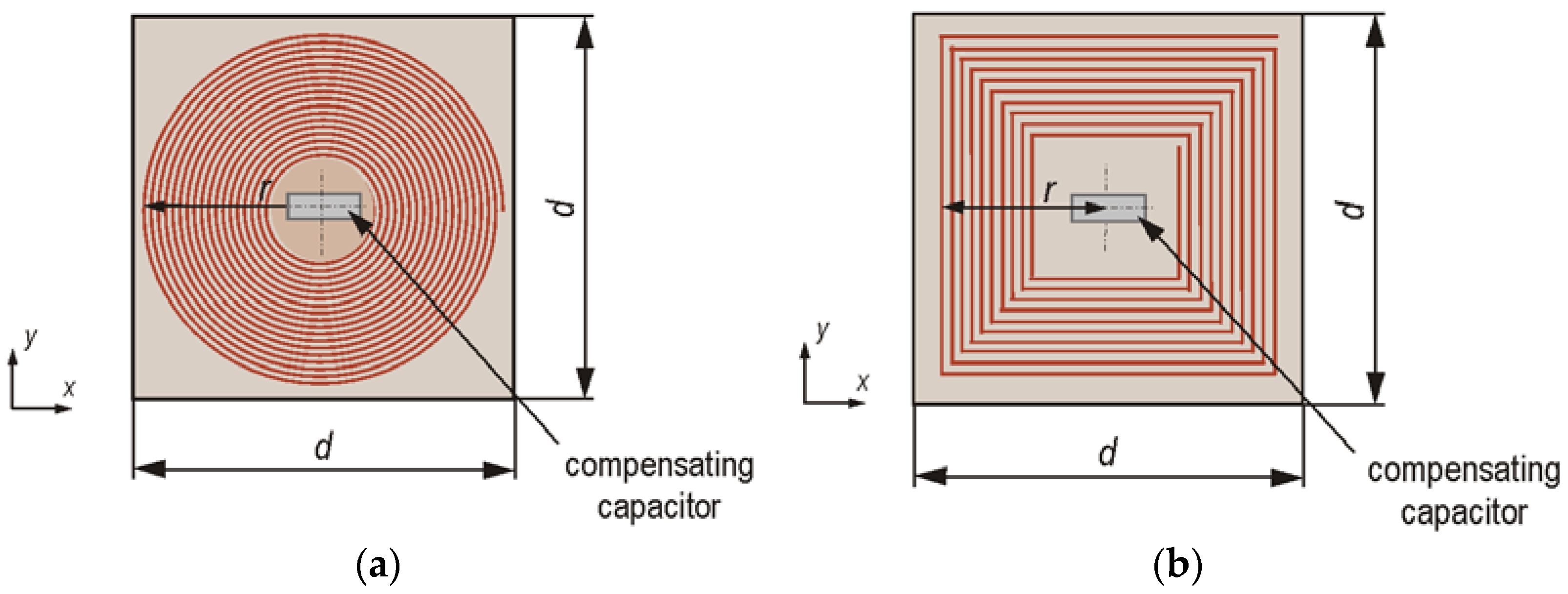
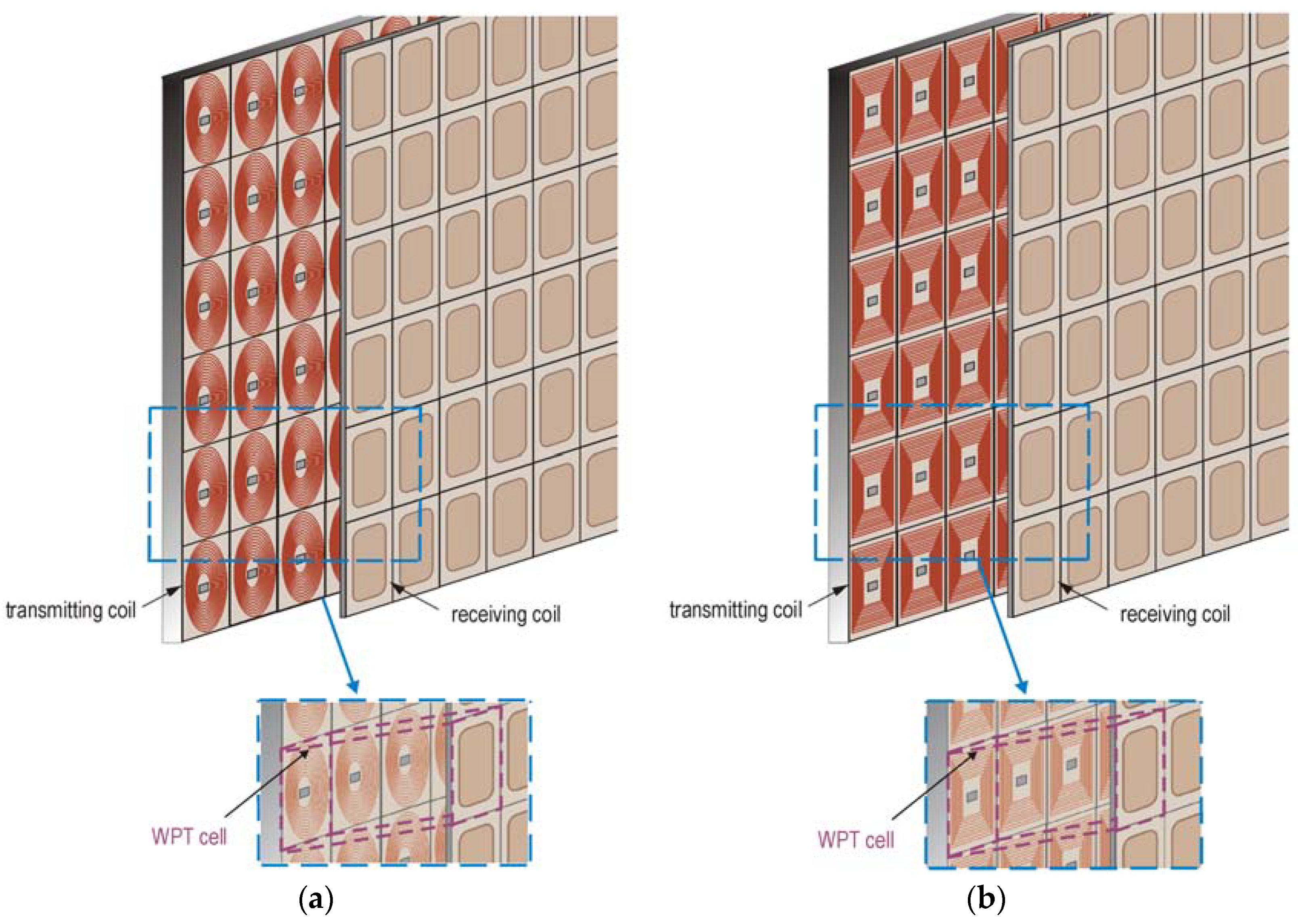
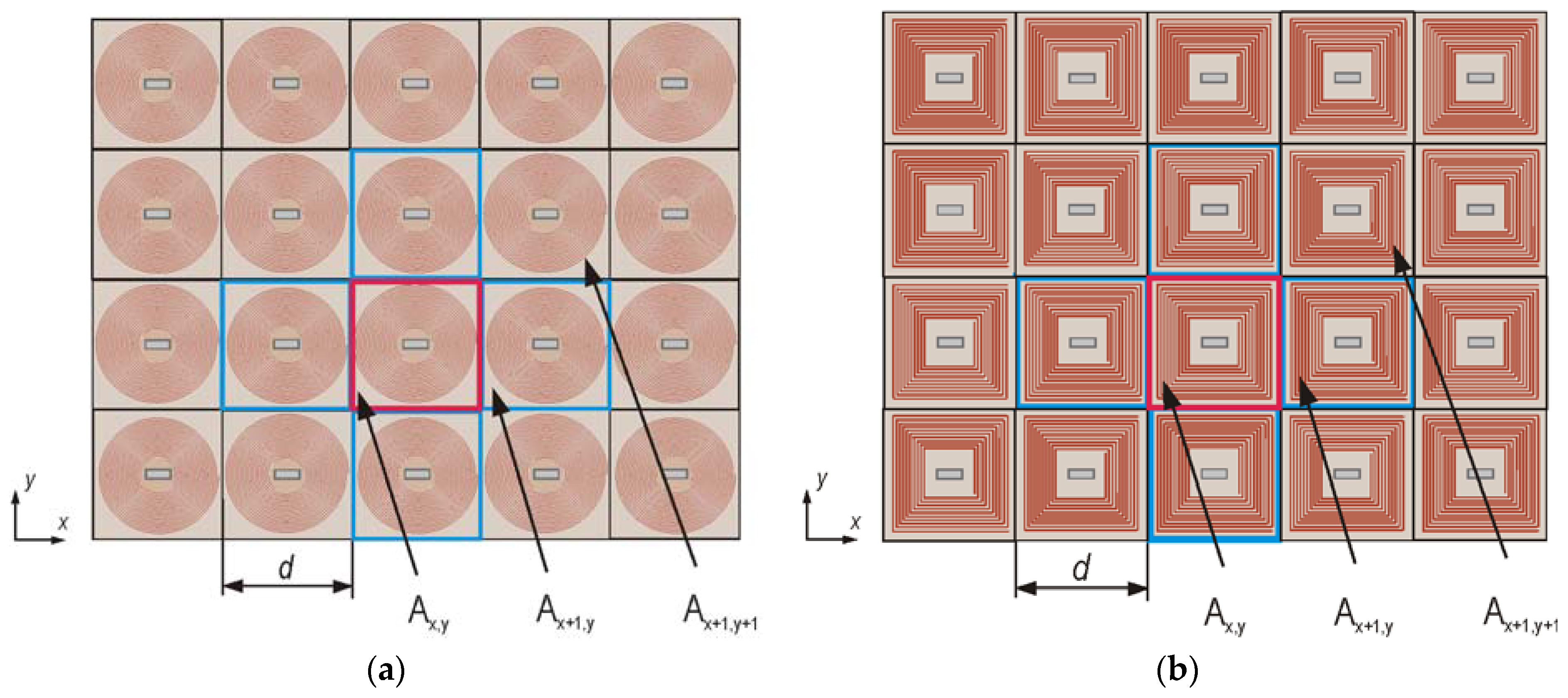
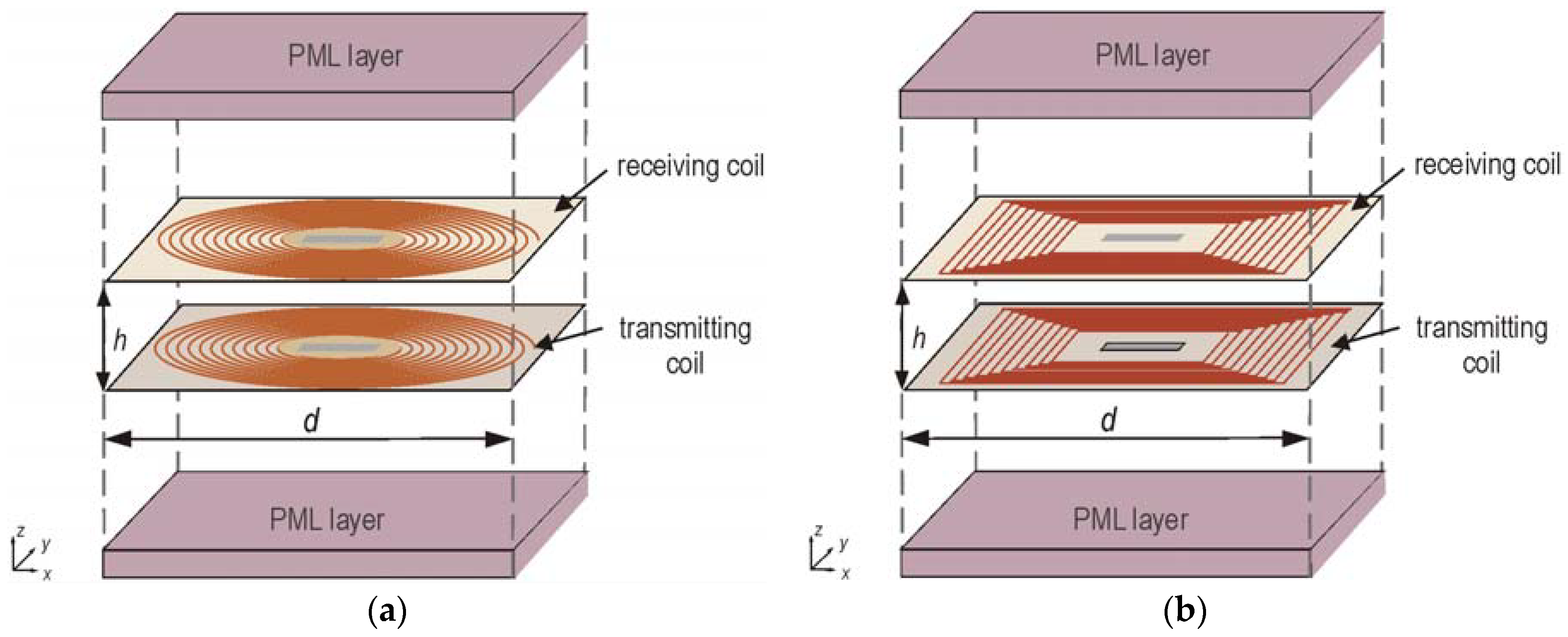
2.1. Description of the Analyzed Models of Wireless Power Transfer System

The analyzed WPT system is composed of periodically arranged pairs of transmitting (Tx) and receiving (Rx) coils. Each pair is called the WPT cell with outer dimensions d × d (Figure 1). Both planar coils in WPT cell are identical and possess the same radius (r) and number of turns (n) wounded around a dielectric carcass. Each coil has an additional compensating capacitor. The distribution of WPT cells results in a transmitting surface consisting of many Tx and sinusoidal voltage source (U_t), while the Rx coils of a receiving surface are connected to loads (Z_l).

Two models of WPT system were analyzed. The first one was made of circular coils with smaller (r = 10 mm) and larger (r = 25 mm) radius (Figure 2a). The second system had identical radii but consisted of square planar coils (Figure 2b). The compensating capacitors were connected in series with the coils.

In the two proposed WPT models, it is possible to select the power conditions in each cell depending on the imposed requirements, e.g., to supply multiple independent receivers simultaneously. The periodic WPT structure consists of two main surfaces: transmitting and receiving, presented in Figure 3. Each surface (composed of Tx or Rx coils) includes a group of planar coils with the same winding direction. The considered cell A_x+j,y+k is an element of an array with identical inductors, where j is the number of column and k is the number of row in a grid (j, k ∈ N and N is the group of integers). Adjacent coils of the element A_x,y (e.g., A_x+1,y or A_x+1,y+1) are separated by the distance d where d ≈ 2r.

Every transmitter Tx is connected in parallel with a sinusoidal voltage source (U_t). The coils creating the receiving surface are linked to a separate load (Z_l). The discussed models of the WPT system guarantee an increase in density of transmitted power in the area between the receiving and transmitting surfaces. This approach also allows the selection of power conditions depending on the requirements.

2.2. Numerical Approach to the Analysis of the Periodic WPT System

The proposed WPT systems were analyzed by using two approaches: 3D numerical model and equivalent circuit. The usage of simpler circuit model renders it possible to easily determine power flow at the design stage or initial analysis of the WPT system. Numerical methods (e.g., FEM, FDTD and FDFD) [35,36,37] allow for the creation of a complex model and determination of the magnetic field distribution. In this typical approach, it is necessary to prepare the 3D model and to impose suitable boundary conditions. However, the efficiency and accuracy of the solution depends on the model size (number of degrees of freedom, NDOF). Increasing NDOF will result in greater accuracy of the solution but also longer computation time. For an open boundary problem, the compromise between numerical methods and circuit approaches is the partial equivalent electrical circuit method (PEEC) [38,39]. It permits modeling geometry and analyzing electric and magnetic phenomena, however, NDOF is significantly reduced due to partitioning of the 3D structure by using larger and, thus, fewer finite elements, which become the coupled nodes in a peculiar kind of electrical circuit [39]. Then, lumped parameters, e.g., self-inductance, mutual inductance and resistance are calculated by an application of integral form of Maxwell’s equations instead of their differential form typical for FDTD or FEM.

The proposed numerical analysis of the system composed of many WPT cells requires taking into account the following: coil geometry (size and shape), number of turns (n), number of WPT cells and elements of the electrical circuit connected to each coil. The wounds of coils can be made of an ultra-thin wire with diameter (w) and covered with insulation of a thickness (i). A compensating capacitor can be modeled as an element with lumped capacity (C) in series with an inductor. The voltage source with given amplitude (U_t) and specified frequency (f) is connected with Tx coil, while the load (Z_l) is connected with Rx coil.

In order to reduce the model to the single cell A_x,y filled with air and containing only a pair of Tx and Rx coils (Figure 4), an infinite array of resonators was modeled by using periodic boundary conditions (PBC) [36,37] imposed on the four lateral surfaces of the cell. A perfectly matched layer (PML) was placed at the top and bottom of the model to imitate an infinite dielectric background. The model was made in the Comsol Multiphysics software. We have performed an analysis in the frequency domain, utilizing Magnetic fields physics in conjugation with the fragmentary Equivalent circuit. The coils were modeled by using a built-in current sheet approximation of the planar inductors (Multi-turn coil boundary condition), while the lumped voltage source (U_t), capacitors (C) and load (Z_l) were attached to the coils by internal coupling with fragmentary Equivalent circuit. NDOF varied for different cases from 200.000 to 400.000 degrees of freedom.

The energy transport in the presented model and the magnetic field phenomena in the frequency domain can be solved by using the Helmholtz equation:

$$\nabla \times \left({\mu }_0^{-1}\nabla \times A\right)-\mathrm{j}\omega \sigma A=J_{ext}$$

(1)

where A denotes magnetic vector potential (Wb/m), ω denotes angular frequency (rad/s), μ₀ denotes permeability of an air (H/m), σ denotes electrical conductivity (S/m), and J_ext denotes external current density (A/m²). Periodic boundary conditions on four external surfaces were defined as magnetic insulation:

$$n_{surf}\times A=0,$$

(2)

where n_surf is the surface normal vector.

The external current density (J_ext) results from the value of the voltage supply (U_t) connected to the transmitting coil. Equation (1) with Equation (2) and PML conditions can be solved by using the Finite Element Method (FEM) [37]. The aim is to find the unknown spatial distribution of the magnetic vector potential A in 3D Cartesian space at specified frequency f.

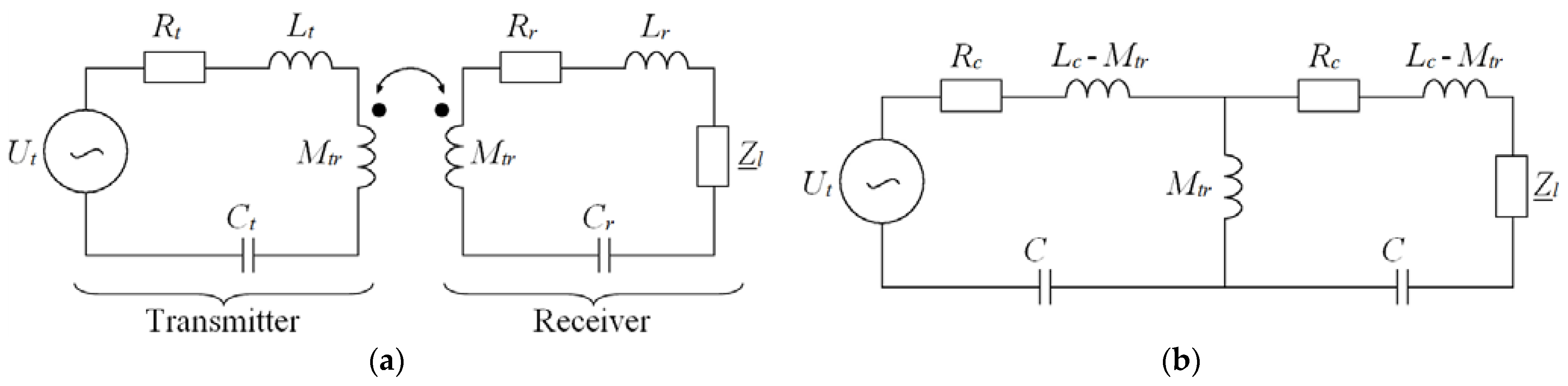
2.3. Analytical Approach to the Analysis of WPT System

Despite the availability of the computational units, it is always a more difficult task to make and solve the numerical model than the equivalent circuit in which there is no need to use boundary conditions. Therefore, in many cases, a simpler model is more desirable if it still provides a similar scope of analysis but less complexity and much faster modeling and calculation processes. Based on the proposed structure of WPT system, two grids (transmitting and receiving surface) with an infinite number of identical resonators have to be considered. In the electrical circuit, the analysis of the infinite periodic network can be reduced to the single cell A_x,y.

The system included identical coils stacked coaxially at the distance h, and they are made of thin wire with electrical conductivity σ. The length of all windings in the circular coil is described by Equation (3), while of the square coil is described by Equation (4)

$$l_{sum,c}=2\pi n\left[r-0.5\left(n-1\right)\left(w+i\right)\right],$$

(3)

$$l_{sum,s}=4n\left[2r-n\left(w+i\right)\right].$$

(4)

If Tx and Rx coils are identical, then their resistances are equal; thus, R_t = R_r = R_c. Taking into account Equation (3), the formula for the resistance R_c of circular coil is as follows.

$$R_c=\frac{l_{sum,c}}{\sigma \pi w^2/4}=\frac{8\pi n\left[r-0.5\left(n-1\right)\left(w+i\right)\right]}{\sigma \pi w^2},$$

(5)

Based on Equation (4), the R_c of the square coil is as follows.

$$R_c=\frac{l_{sum,s}}{\sigma \pi w^2/4}=\frac{16n\left[2r-n\left(w+i\right)\right]}{\sigma \pi w^2}.$$

(6)

In an infinite periodic grid where each coil has identical electrical parameters and magnetic coupling occurs with its neighbors, it is possible to reduce an analysis to the single WPT cell (Figure 5). Mutual inductances between coil in the cell A_x,y and coils in cells A_x+i,y+j affect the internal inductance of the coil in A_x,y, which can be expressed for both types of the coils as follows.

$$L_c=L_{self}+{\displaystyle \sum _i{\displaystyle \sum _j\left(M_{x+i,y+j}\right)}},$$

(7)

The following components of Equation (7) are as follows: L_c—effective inductance in (H); M_x+i,y+j—mutual inductance in (H) between coils adjacent in horizontal plane, for i ≠ 0 and j ≠ 0; L_self—self-inductance of the planar coil in (H).

Self-inductance is calculated using equation [40]:

$$L_{self}=\frac{{\mu }_0{c}_1{d}_m{n}^2}{2}\left[\ln \left(\frac{c_2}{\nu }\right)+c_3\nu +c_4{\nu }^2\right],$$

(8)

where d_m is mean diameter and ν is a fill coefficient.

$$d_m=2r-n\left(w+i\right),$$

(9)

$$\nu =\frac{n\left(w+i\right)}{2r-n\left(w+i\right)}.$$

(10)

In Equation (8) coefficients c₁, c₂, c₃ and c₄ are dependent on the shape of the coil [40]. The values of the coefficients for circular and square inductors are presented in

Table 1. Geometrical coefficients for circular and square coils [40].

Type of Coil	Coefficient
	c1	c2	c3	c4
Circular coil	1.0	2.5	0	0.2
Square coil	1.46	1.9	0.18	0.13

.

From Equation (7), an inductance of the considered coil in a segment A_x,y takes the following form:

$$L_c=L_{self}-M_{pe},$$

(11)

where M_pe is sum of mutual inductances in the periodic grid. Since these mutual inductances reduce the effective inductance of the coil, the inductance M_pe is written with a minus. For the case when loads Z_l = ∞ and there is no capacitor in series with Tx coils, at the arbitrary frequency f, one may find M_pe as follows [11]:

$$M_{pe}=\frac{\left|\frac{U_t}{{\underset{\_}{I}}_{t,\infty }}-R_c\right|}{2\pi f}-L_{self},$$

(12)

where I_t,∞=|I_t,∞|e^jψ is the source current in (A); |I_t,∞| is the RMS value of the source current in (A); ψ is the phase angle between the source voltage and current in (rad). The underlined quantities, e.g., the current I_t,∞ in Equation (12), denotes the complex number.

According to the equivalent circuit shown in Figure 5b, instead of calculating inductances M_tr,x+i,y+j, the mutual inductance M_tr between Tx and Rx can be found as [11].

$$M_{tr}=\left|\frac{{\underset{\_}{U}}_{r,\infty }}{2\pi f{\underset{\_}{I}}_{t,\infty }}\right|,$$

(13)

where U_r,∞=|U_r,∞|e^jθ is the voltage induced in the receiving coil in (V), |U_r,∞| is the RMS value of the induced voltage in (V) and θ is the phase angle between the source voltage and induced voltage in (rad).

After calculations of self-inductance (L_self), mutual inductance of periodically adjacent coils (M_pe) and mutual inductance between Tx and Rx (M_tr), it is possible to find the compensating capacity (C) at a specified frequency.

$$C\left(f\right)=\frac{1}{4{\pi }^2{f}^2{L}_c}=\frac{1}{4{\pi }^2{f}^2\left(L_{self}-M_{pe}\right)}.$$

(14)

3. Analytical and Numerical Results

3.1. Analyzed Models

By the utilization of the proposed analytical and numerical models, many variants of the periodic WPT system were analyzed (

Table 2. Geometrical parameters of the two types of the analyzed coils.

r (mm)	n	h (mm)
		0.5 r	r
10	15	5.0	10.0
	25	5.0	10.0
	35	5.0	10.0
	45	5.0	10.0
25	40	12.5	25.0
	50	12.5	25.0
	60	12.5	25.0
	70	12.5	25.0
	80	12.5	25.0

). The shapes of the coils (circular or square), radius (r), number of turns (n) and distance between Tx and Rx coils (h) were changed.

Based on the results obtained for several exemplary periodic WPT systems, the correctness of the proposed analytical model was verified by comparing the active power of the receiver:

$$P_o=Z_l{\left|{\underset{\_}{I}}_r\right|}^2,$$

(15)

where I_r is the current flowing through receiving coil in (A). The power of the transmitter is represented by the following:

$$P_z=U_t{\underset{\_}{I}}_t,$$

(16)

where I_t is the current flowing through transmitting coil in (A). By using Equations (15) and (16), the power transfer efficiency was calculated as follows.

$$\eta =\frac{P_o}{P_z}100\%.$$

(17)

The comparison concerned the determination of the powers P_o and P_z and also efficiency η. Additionally, the analysis was divided into two cases:

-

Operation with maximum efficiency, where the optimal load impedance was described as follows.

$$Z_e=\sqrt{R_c{}^2+{\left(2\pi f{M}_{tr}\right)}^2},$$

(18)

-

Operation with maximum transferred power, where the optimal load impedance was described as follows.

$$Z_p=R_c+\frac{{\omega }^2{M}_{tr}{}^2}{R_c}.$$

(19)

The discussed unit cell A_x,y was subjected to analysis where it was assumed that the system was made of the infinite number of WPT cells. Each WPT cell consisted of pair of identical coaxial coils (Tx and Rx). The parameters regarding windings (wires) of the coils, which were used in models, are presented in

Table 3. Parameters of the wire used to form the coils.

Parameter	Symbol	Value
Diameter of the wire	w	200 µm
Thickness of the wire insulation	i	5 µm
Conductivity of the wire (copper)	σ	5.6 × 107 S/m

. The analysis was performed in the frequency domain for the frequencies from f_min = 100 kHz to f_max = 1000 kHz. The amplitude of the voltage source was set to U_t = 1 V.

The numerical model was created in the Comsol Multiphysics software and was solved by using FEM. We utilized built-in, multi-turn coils approximation (current sheet approximation) and the electrical circuit connected with the 3D model. The lumped parameters of the electrical circuit from Figure 5b (

Table 4. Self and mutual inductances as well as compensating capacities and load impedance (at f_max) for circular coils and r = 10 mm.

n	Lself (μH)	C at fmax (nF)	Ze (Ω) at fmax		Zp (Ω) at fmax		Mtr (μH)
			h = 0.5 r	h = r	h = 0.5 r	h = r	h = 0.5 r	h = r
15	6.29	5.07	5.27	1.28	61	3.56	0.84	0.19
25	11.72	2.64	12.23	2.90	222	12.53	1.94	0.45
35	15.40	1.96	17.46	4.12	374	20.81	2.78	0.64
45	16.70	1.79	19.12	4.49	414	22.84	3.04	0.70

,

Table 5. Self and mutual inductances as well as compensating capacities and load impedance (at f_max) for circular coils and r = 25 mm.

n	Lself (μH)	C at fmax (pF)	Ze (Ω) at fmax		Zp (Ω) at fmax		Mtr (μH)
			h = 0.5 r	h = r	h = 0.5 r	h = r	h = 0.5 r	h = r
40	107	293	93	21.37	2881	152	14.79	3.37
50	143	219	137	31.54	5219	279	21.71	4.99
60	175	178	180	41.71	7951	428	28.59	6.61
70	204	154	218	50.75	10627	575	34.73	8.04
80	227	139	249	57.78	12798	691	39.56	9.16

,

Table 6. Self and mutual inductances as well as compensating capacities and load impedance (at f_max) for square coils and r = 10 mm.

n	Lself (μH)	C at fmax (nF)	Ze (Ω) at fmax		Zp (Ω) at fmax		Mtr (μH)
			h = 0.5 r	h = r	h = 0.5 r	h = r	h = 0.5 r	h = r
15	8.33	4.73	4.26	1.03	31.41	1.85	0.67	0.14
25	15.22	2.45	11.24	2.59	149	7.94	1.78	0.39
35	19.66	1.82	16.98	3.94	283	15.17	2.70	0.60
45	20.95	1.66	18.93	4.38	325	17.43	3.01	0.68

and

Table 7. Self and mutual inductances as well as compensating capacities and load impedance (at f_max) for square coils and r = 25 mm.

n	Lself (μH)	C at fmax (pF)	Ze (Ω) at fmax		Zp (Ω) at fmax		Mtr (μH)
			h = 0.5 r	h = r	h = 0.5 r	h = r	h = 0.5 r	h = r
40	142	277	76	15.97	1507	67	12.03	2.47
50	187	205	118	25.52	3106	144	18.84	4.00
60	228	164	164	36.01	5222	252	26.07	5.67
70	264	140	207	46.15	7556	375	32.94	7.29
80	292	124	244	54.76	9716	491	38.77	8.66

) for circular and square coils were found using preliminary numerical calculations and Equations (8), (13), (14), (18) and (19).

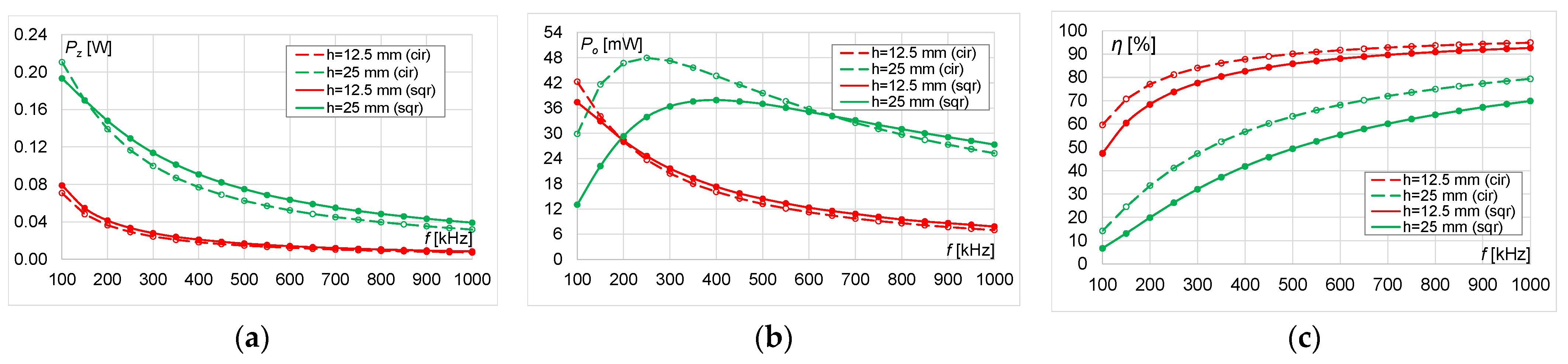
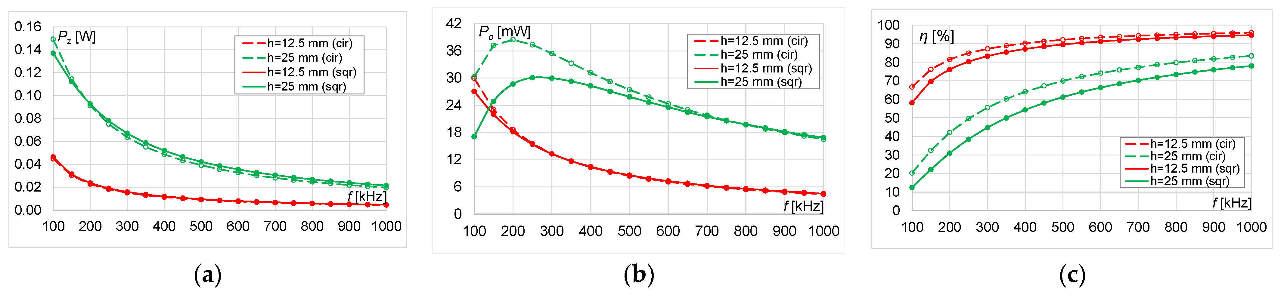
3.2. System Operating with Maximum Efficiency

The calculation results of the proposed WPT system, received by the numerical and analytical method, were compared. The structure of the WPT system was taken into account (radius and shape of the coil, number of turns and distance between coils), and the transmitter and receiver powers were calculated based on both analytical and numerical models.

The first operating mode was related with maximum efficiency. Impedances of the load (Z_e) were calculated based on Equation (18) for different number of turns and distance between Tx and Rx and presented in Figure 6 for the coil with r = 10 mm and in Figure 7 for the coil with r = 25 mm. The analysis showed that the values of impedances (Z_e) were always higher for the circular coil. An increase in the number of turns causes a nonlinear increase in the impedance. Doubling the distance h results in an over four times decrease in the impedance for both coil sizes and types of the coils.

In

Table 8. A list of maximum values of power transfer efficiency at f_max for all calculated cases.

n	η (%) at fmax
	Circular Coil		Square Coil
	h = 0.5 r	h = r	h = 0.5 r	h = r
15 (r = 10 mm)	83.99	47.16	76.12	28.32
25 (r = 10 mm)	89.57	62.36	86.00	50.79
35 (r = 10 mm)	91.09	66.97	88.66	58.81
45 (r = 10 mm)	91.18	67.15	88.99	59.81
40 (r = 25 mm)	93.75	75.37	90.44	61.55
50 (r = 25 mm)	94.90	79.68	92.65	69.92
60 (r = 25 mm)	95.58	82.39	93.92	75.01
70 (r = 25 mm)	95.98	83.77	94.67	78.10
80 (r = 25 mm)	96.19	84.57	95.11	79.92

, the maximum power transfer efficiency values depending on the type of the coils, the number of turns and the distance between Tx and Rx were compared. In each case, higher power transfer efficiency values were obtained for the circular coil than for the square one.

In order to compare the results obtained with the analytical and numerical methods, the calculated absolute error is shown in

Table 9. Values of absolute error calculated for power transfer efficiency at all frequencies and cases.

n	δ (%)
	Circular Coil		Square Coil
	h = 0.5 r	h = r	h = 0.5 r	h = r
15 (r = 10 mm)	0.16	0.17	0.02	0.01
25 (r = 10 mm)	0.13	0.07	0.02	0.02
35 (r = 10 mm)	0.14	0.19	0.01	0.02
45 (r = 10 mm)	0.19	0.11	0.01	0.02
40 (r = 25 mm)	0.02	0.37	0.00	0.02
50 (r = 25 mm)	0.01	0.30	0.01	0.02
60 (r = 25 mm)	0.04	0.13	0.01	0.02
70 (r = 25 mm)	0.06	0.27	0.01	0.02
80 (r = 25 mm)	0.04	0.40	0.01	0.02

. The results are consistent and do not exceed 0.4%.

The exact characteristics of the source power, receiver power and power transfer efficiency are presented on the graph in the following subsections: small cell (r = 10 mm) in Section 3.2.1 and large cell (r = 25 mm) in Section 3.2.2. The results of the numerical analysis are shown as dashed lines for circular coils and solid lines for square coils. The results of the analytical analysis, based on the previously presented formulas (Section 2.3), are marked with dots for each type of the coil and the distance between Tx and Rx.

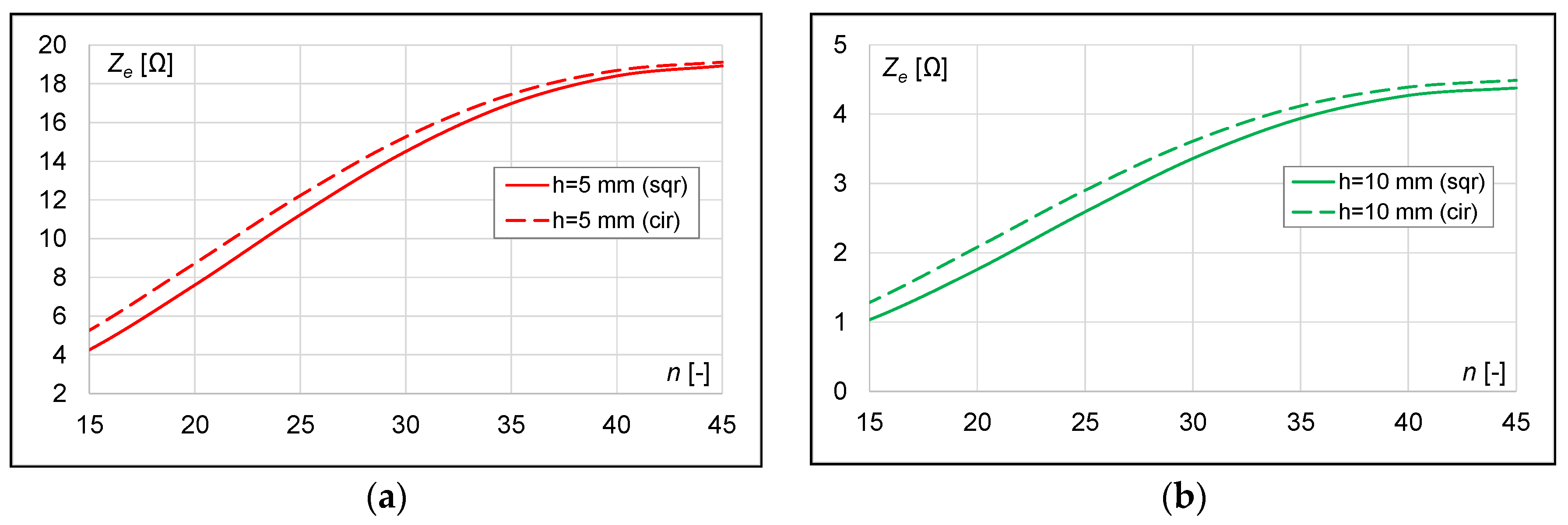
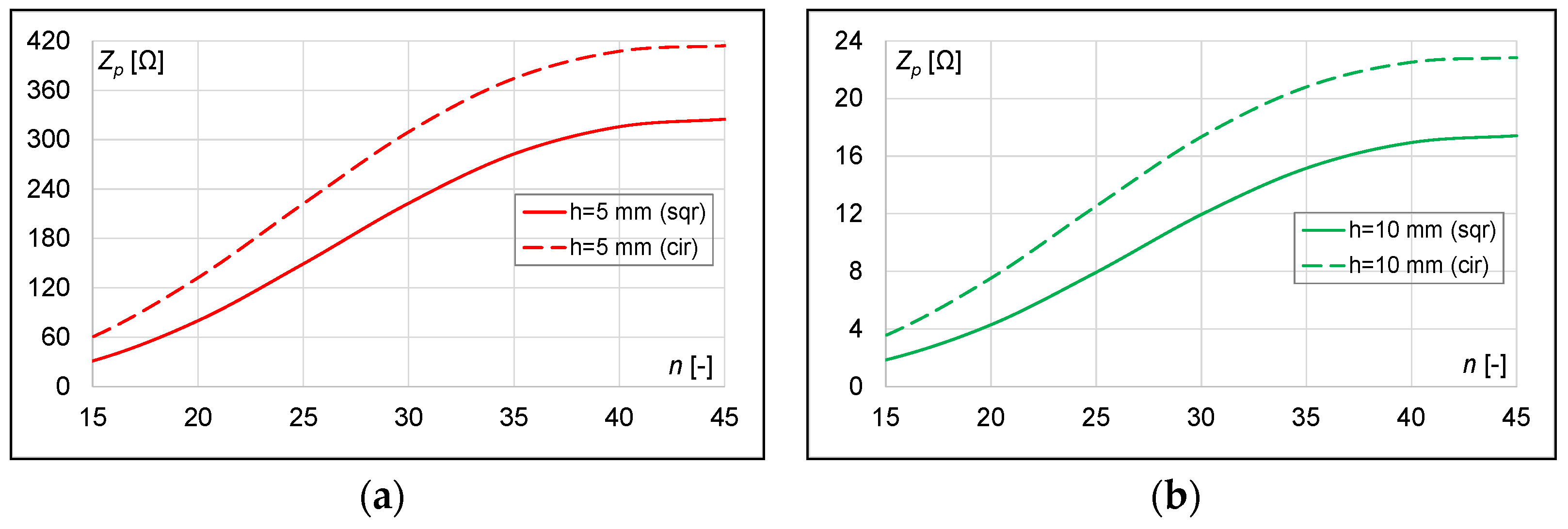
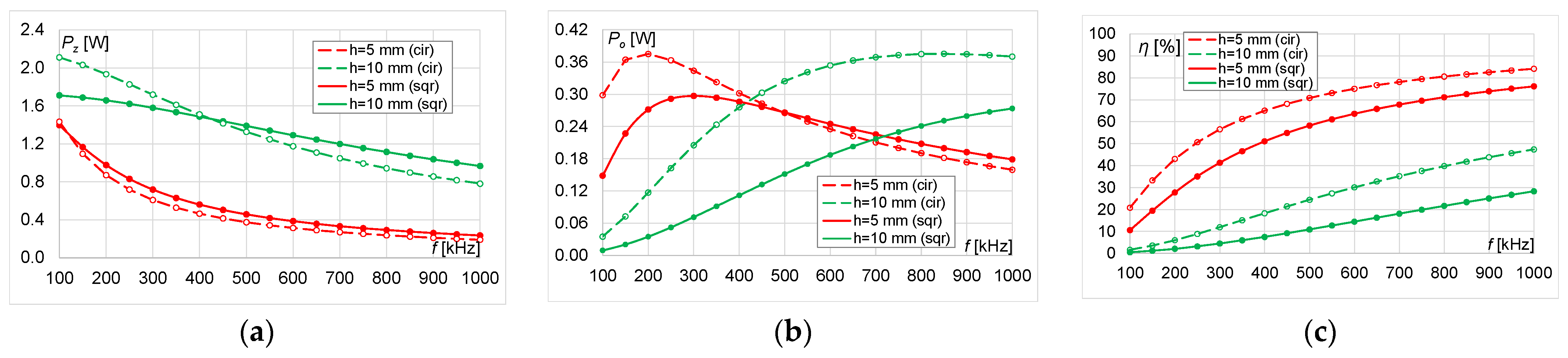
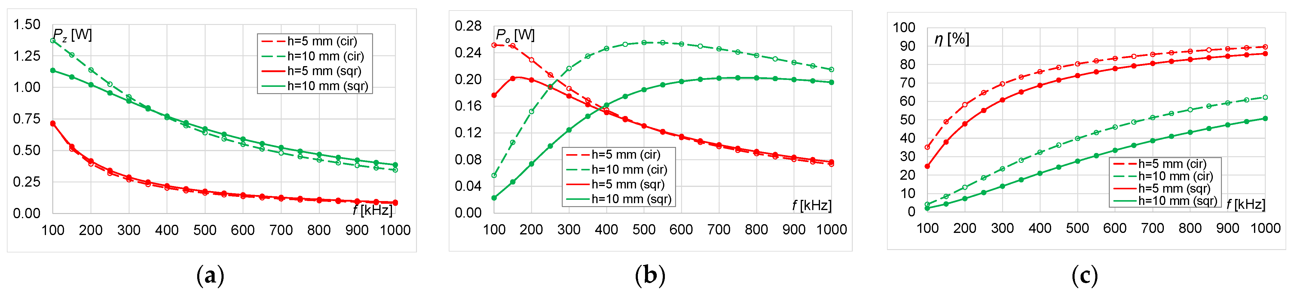
3.2.1. Maximum Power Transfer Efficiency for Small Coil (r = 10 mm)

Figure 8, Figure 9, Figure 10 and Figure 11 show the characteristics of the following: power (transmitter and receiver) and efficiency at the distance h = r/2 = 5 mm and h = r = 10 mm between coils for circular and square planar spiral coils.

The transmitter power (P_z) decreases over the entire frequency range, regardless of the type and size of the coil and the number of turns (Figure 8a, Figure 9a, Figure 10a and Figure 11a). The transmitter power is almost the same for the circular and square coil at the distance h = r/2. For the distance h = r, P_z is greater for the circular coil in the initial frequency range (from 100 kHz to about 450 kHz), and P_z values are greater for the square coil with increasing frequency.

For all characteristics (Figure 8b, Figure 9b, Figure 10b and Figure 11b), it can be noted that when the efficiency reaches approximately 50%, the receiver power (P_o) reaches its maximum value. Then, the receiver power decreases as efficiency exceeded 50%. Despite the nonlinear frequency dependency of power and efficiency, the number of turns also has a significant impact. By increasing the number of turns, the receiver power will fall. The shape of the receiver power characteristics for both types of the coils is very similar. Maximum receiver power is achieved for h = 5 mm in the range 100 kHz ÷ 200 kHz and for h = 10 mm in the range 450 kHz ÷ 800 kHz.

The greatest difference in efficiency between circular and square coils occurs at n = 15 and reaches almost 20% (at f = 1MHz, h = 10 mm) and almost 15% (at f = 300 kHz, h = 5 mm) (Figure 8c). As the number of turns increases, this difference decreases and at n = 45 it does not exceed 8% regardless of the distance between the coils h (Figure 11c). For h = 5 mm and n = 35, the number of turns n = 45 had minor impact on the efficiency, which reached almost 90% at 1 MHz for both types of the coils (Figure 10c and Figure 11c). For h = 10 mm, efficiency reached 67% for circular coils and 60% for square coils (Figure 11c). Doubling the distance between the coils caused the efficiency to decrease by 20–40%.

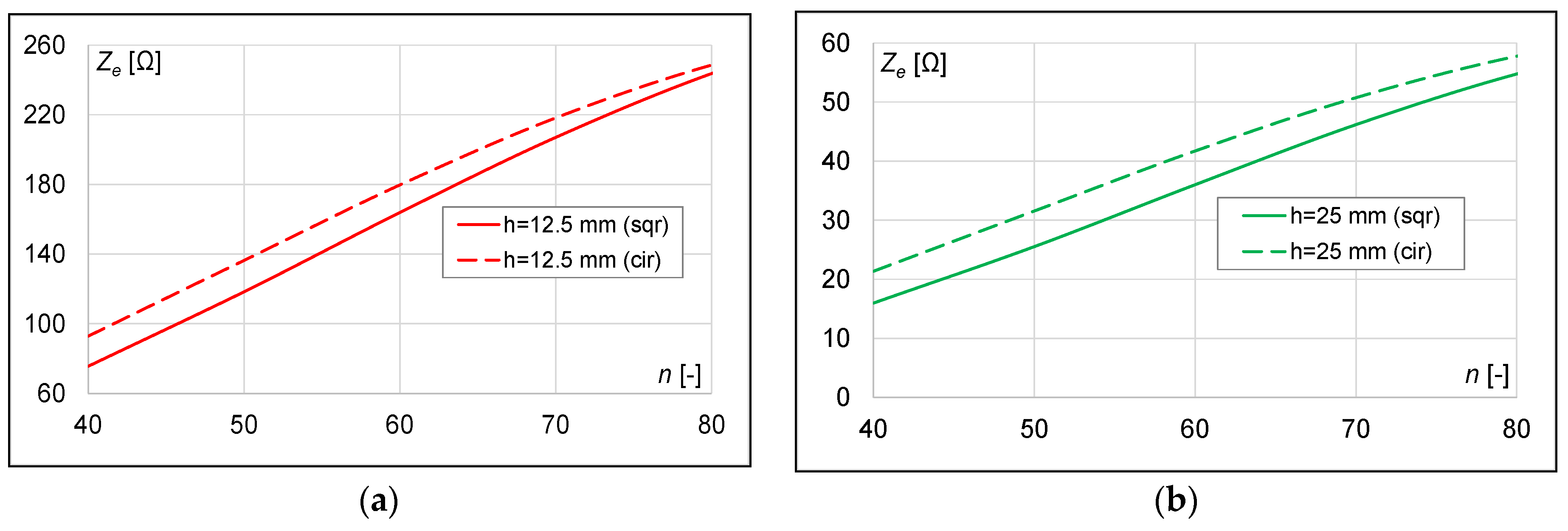
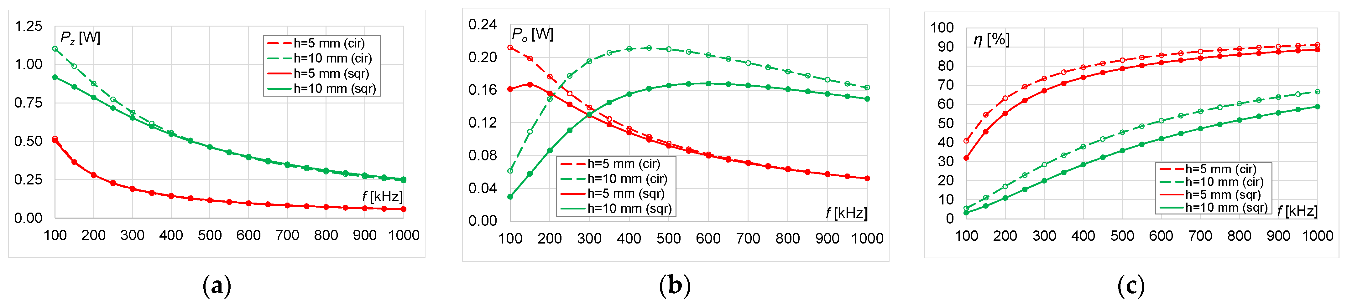
3.2.2. Maximum Power Transfer Efficiency for Large Coil (r = 25 mm)

Figure 12, Figure 13, Figure 14, Figure 15 and Figure 16 show the characteristics of the following: power (transmitter and receiver) and efficiency at the distance h = r/2 = 12.5 mm and h = r = 25 mm for circular and square planar spiral coils.

Regardless of the type of the coil and the number of turns, the transmitter power (P_z) decreases over the entire frequency range (Figure 12a, Figure 13a, Figure 14a, Figure 15a and Figure 16a). For the large coil (r = 25 mm) and the h = 12.5 mm distance between the coils, the transmitter power is almost the same for the circular and square coil. However, for the distance h = 25 mm, P_z is greater for the circular coil in the initial frequency range, and it is greater for the square coil with increasing frequency. For the distance h = r, P_z is greater for the circular coil in the initial frequency range 100 kHz ÷ 300 kHz, and the P_z values became greater for the square coil with increasing frequency.

On all characteristics, it can be noted that when the efficiency reaches approximately 50%, the receiver power P_o reaches its maximum value. Then, the receiver power decreases as efficiency exceeded 50%. Maximum receiver power is achieved for h = 12.5 mm at f = 100 kHz and for h = 25 mm in the range 200 kHz ÷ 250 kHz. For larger distances between coils h = r = 25 mm, the values of the receiver power for the circular coils are greater than for the square coils up to the frequency of about 700 kHz, and the relationship is inverse.

Regardless of the size of the coils, the number of turns and the distance between the coils, the efficiency is always greater for circular coils than for square ones (Figure 12c, Figure 13c, Figure 14c, Figure 15c and Figure 16c). The efficiency of the analyzed system increases with increasing frequency and the number of turns. Regardless of the number of turns, doubling the distance between the coils caused the efficiency to decrease by 20–50% in lower frequency range and by 10–40% in higher frequency range. The greatest differences in efficiency between the circular and square coils occurred at n = 40 and reached almost 20% (h = 25 mm, f = 400 kHz) and almost 15% (h = 12.5 mm, f = 100 kHz) (Figure 12c). For large distances (h = 25 mm), as the number of turns increases, the difference in efficiency between the circular and square coils becomes smaller.

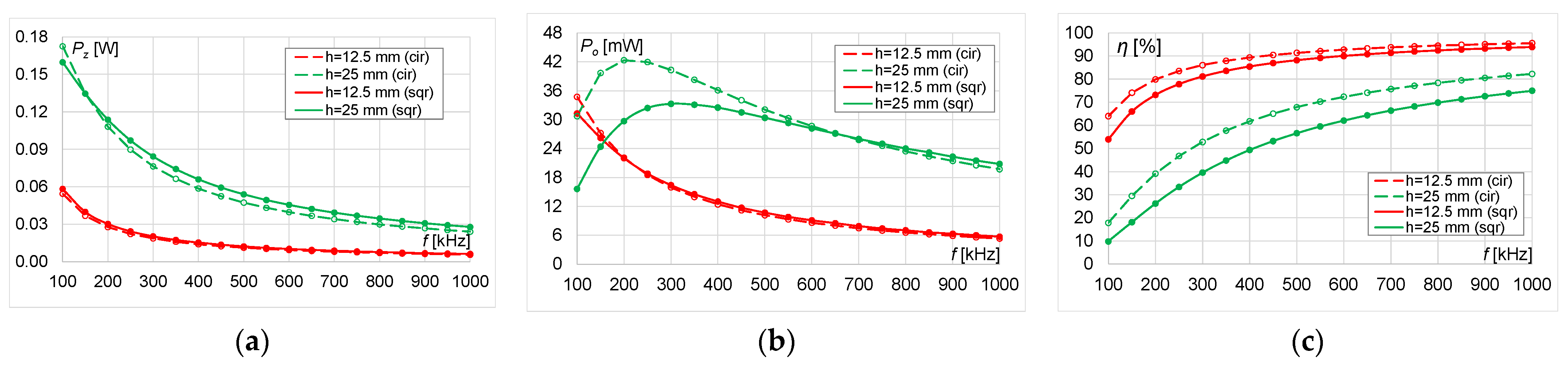
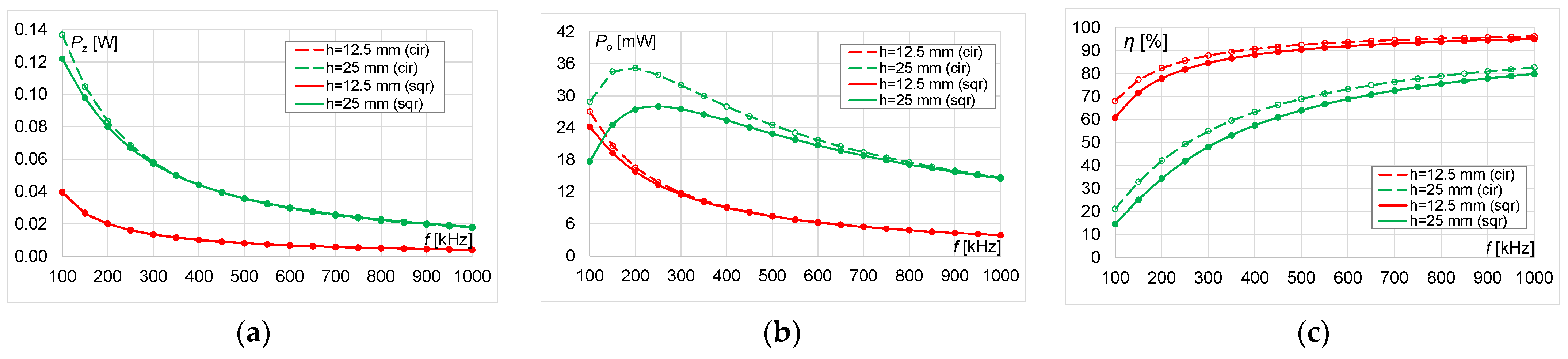
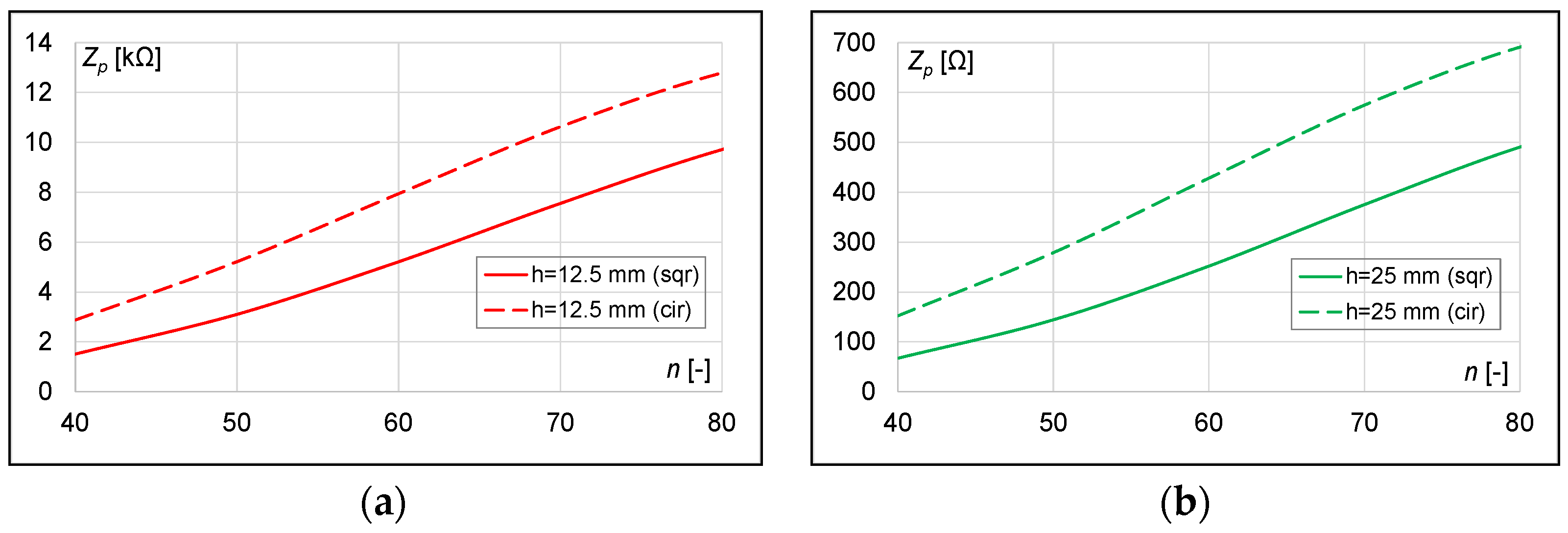
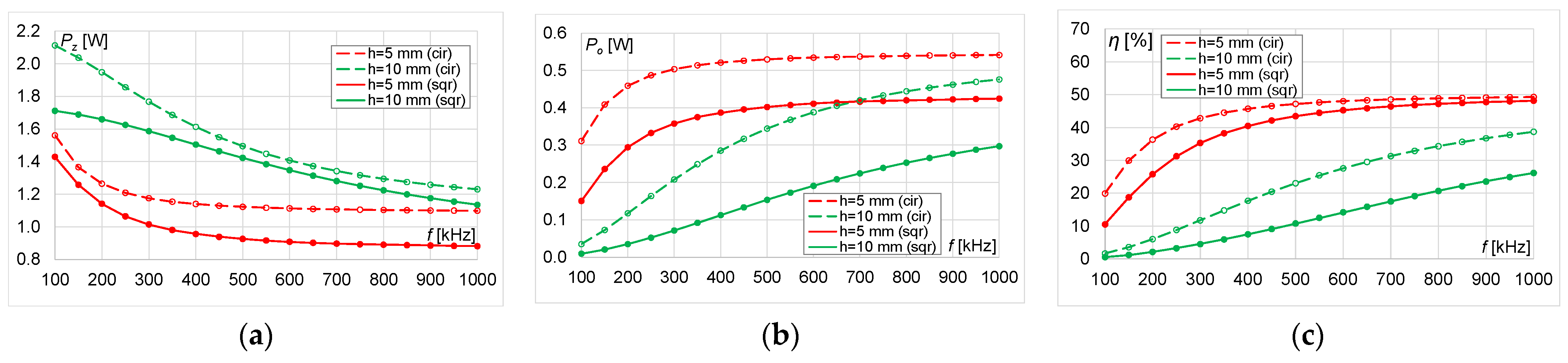
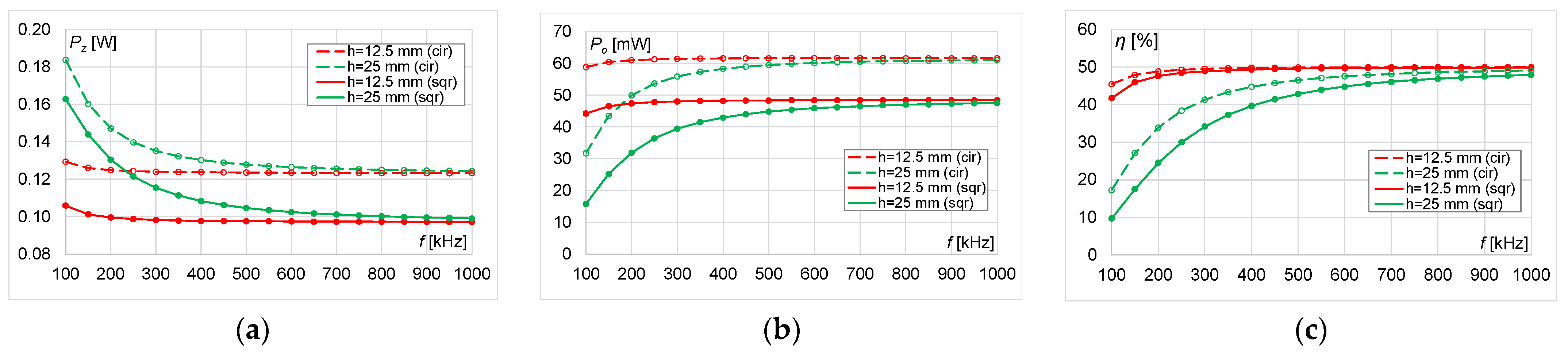
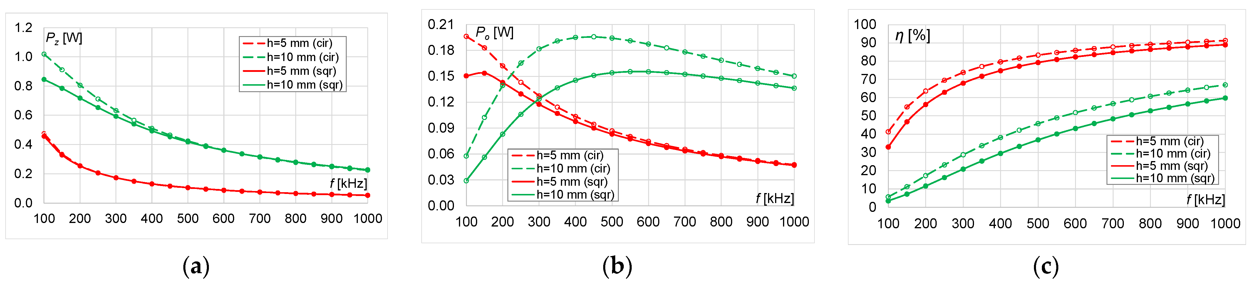
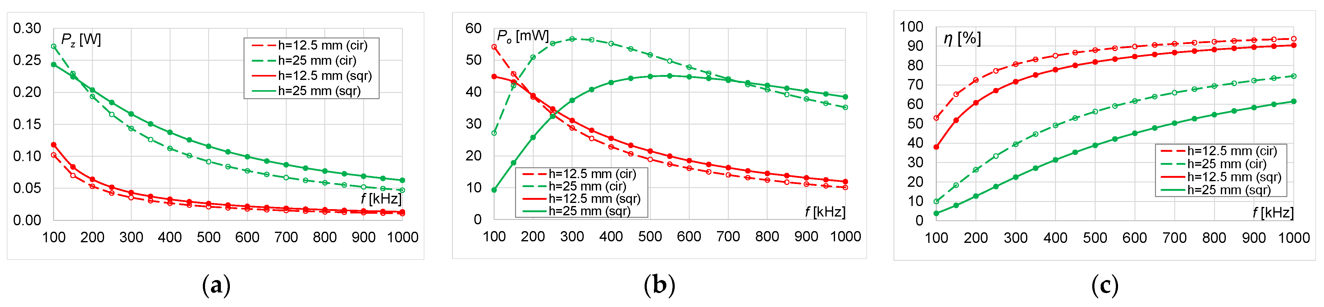
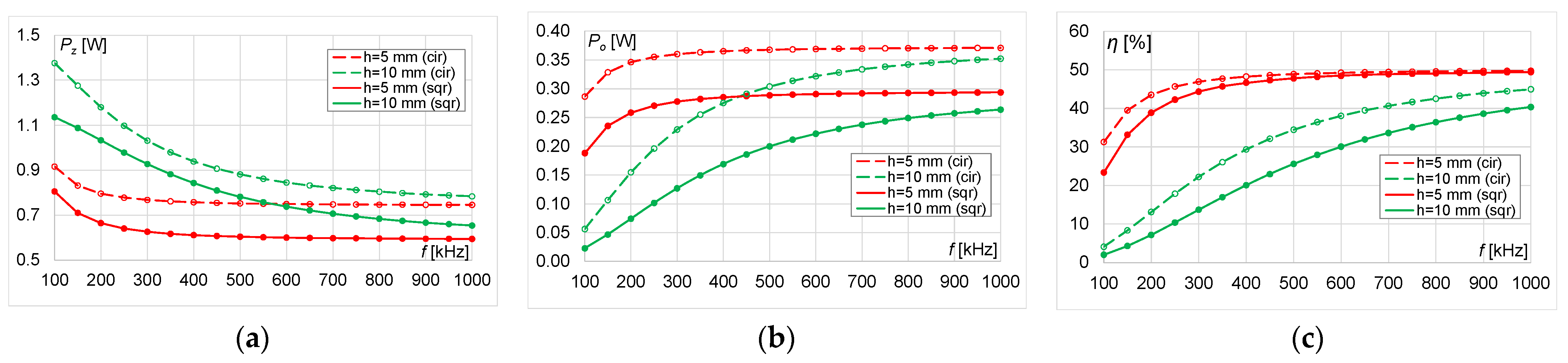
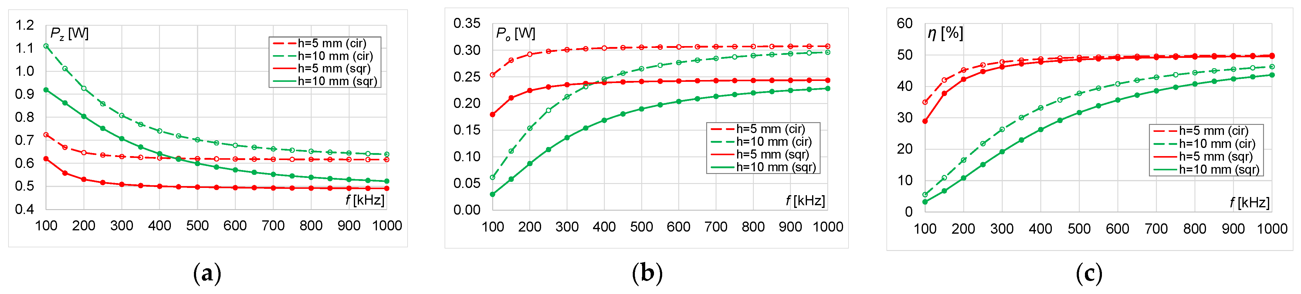
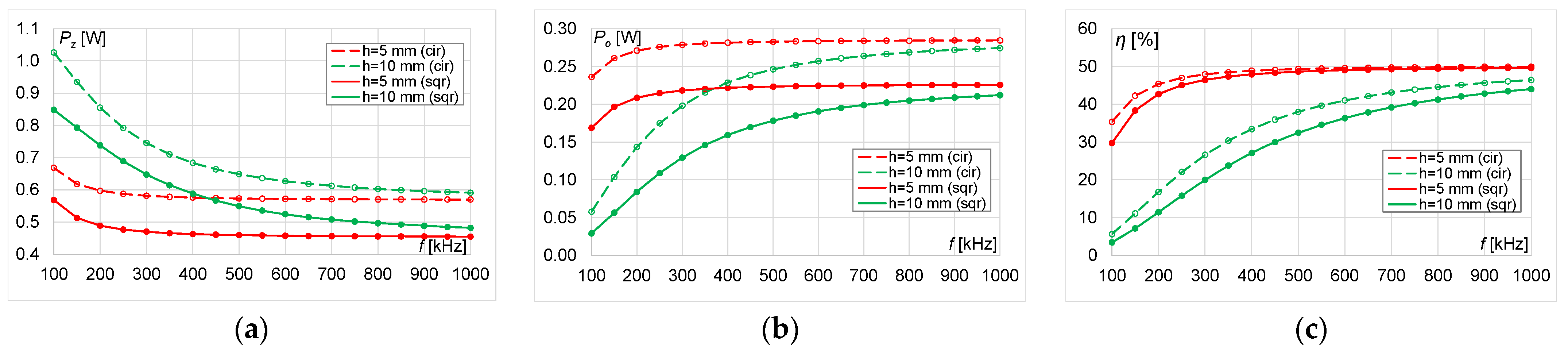
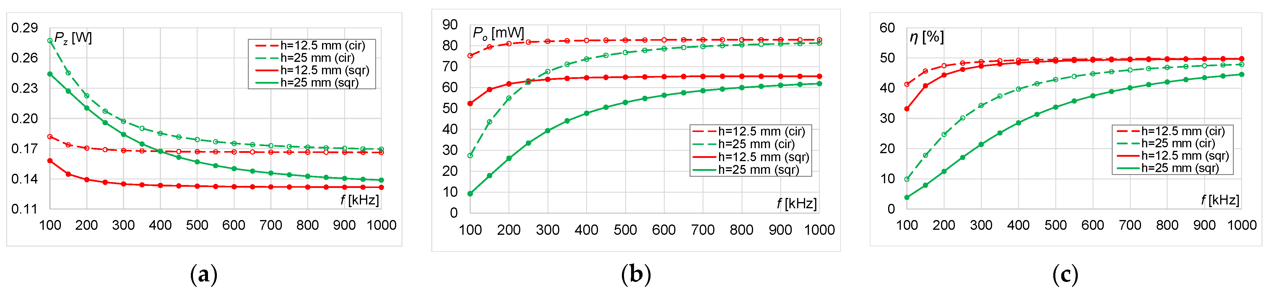
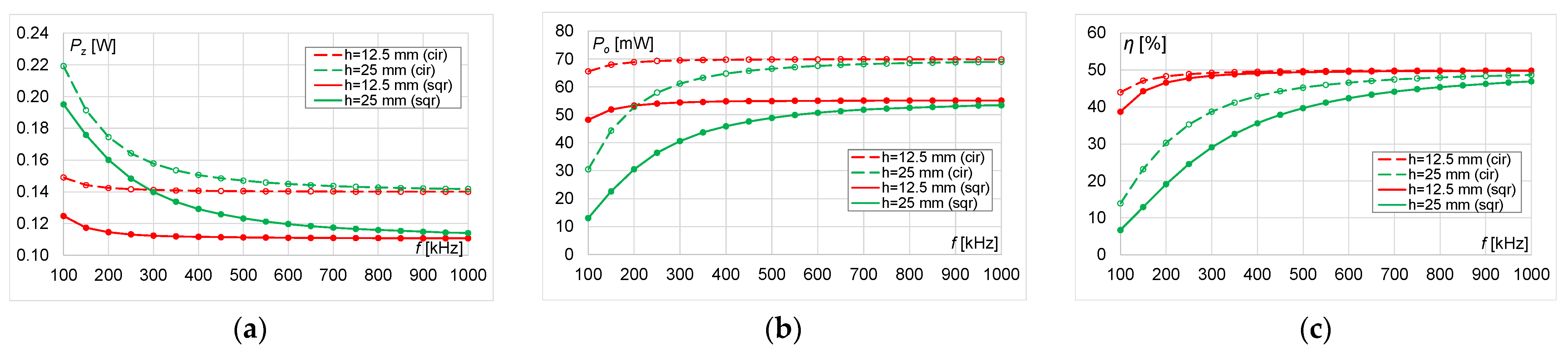
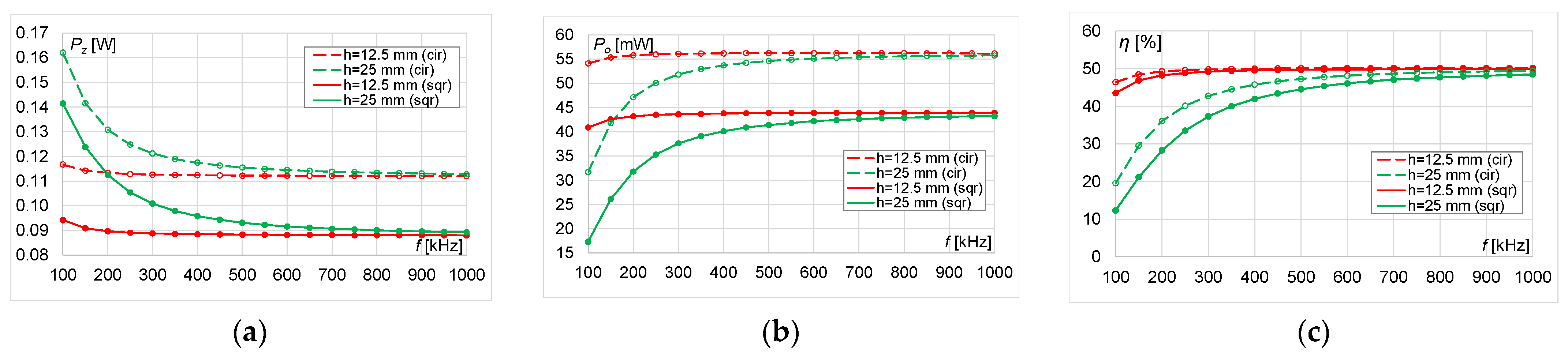
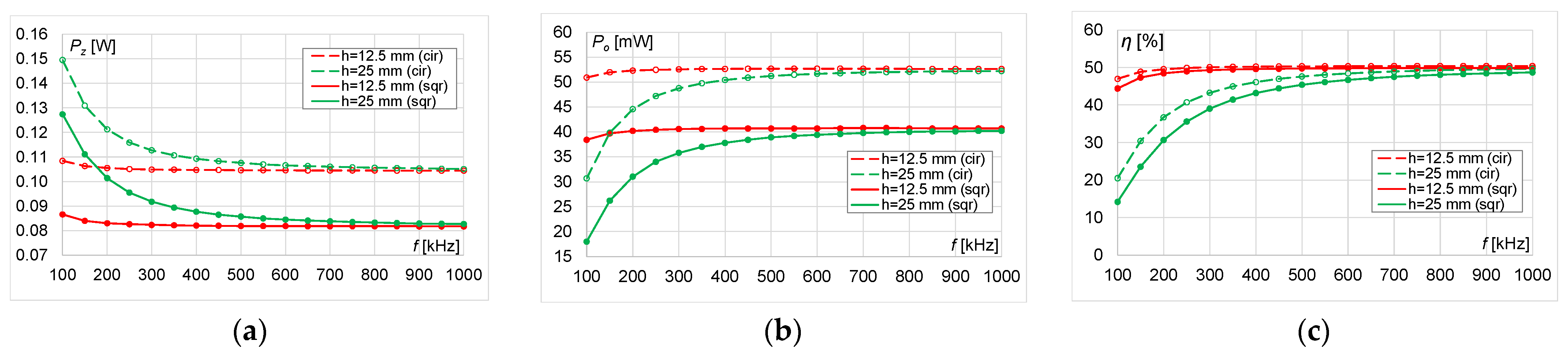
3.3. System Operating with Maximum Load Power

The second operating mode was related with the maximum load power. In order to determine the maximum power transferred to the receiver, the values of load impedance (Z_p) were calculated by taking into account the number of turns, distance between the coils and mutual inductance for circular and square planar spiral coils for the following: r = 10 mm (Figure 17) and r = 25 mm (Figure 18). As with the previous approach (Section 3.2), it can be observed that impedance values are greater for circular coils than square coils. In both types of the coils, doubling the distance h results in an over seventeen-times decrease in the impedance (for r = 10 mm) but more than a twenty-times decrease in Z_p for square coils (for r = 25 mm).

The maximum load power values depending on the type of the coils, the number of turns and the distance (h) are presented in

Table 10. Maximum load power values at f_max for all analyzed cases.

n	Po (mW) at fmax
	Circular Coil		Square Coil
	h = 0.5 r	h = r	h = 0.5 r	h = r
15 (r = 10 mm)	541	475	425	298
25 (r = 10 mm)	370	351	294	264
35 (r = 10 mm)	306	295	244	229
45 (r = 10 mm)	283	272	226	212
40 (r = 25 mm)	83	82	66	62
50 (r = 25 mm)	70	69	55	54
60 (r = 25 mm)	62	61	49	48
70 (r = 25 mm)	56	55	44	43
80 (r = 25 mm)	52	51	41	40

. In each case, higher power transfer efficiency values were obtained for the circular coil than for the square one. The maximum load power at the receiver is about 20% greater for the circular coil than for the square one.

The compared values obtained with proposed circuit and FEM methods were performed by calculation of the absolute error for all frequencies and all cases (

Table 11. Values of absolute error calculated for transferred power.

n	δ (mW)
	Circular Coil		Square Coil
	h = 0.5 r	h = r	h = 0.5 r	h = r
15 (r = 10 mm)	0.88	1.57	0.77	0.46
25 (r = 10 mm)	0.83	1.05	0.41	0.33
35 (r = 10 mm)	1.15	1.21	0.31	0.27
45 (r = 10 mm)	1.99	2.10	0.26	0.25
40 (r = 25 mm)	0.31	0.38	0.10	0.08
50 (r = 25 mm)	0.12	0.14	0.08	0.12
60 (r = 25 mm)	0.15	0.16	0.10	0.09
70 (r = 25 mm)	0.24	0.25	0.08	0.09
80 (r = 25 mm)	0.32	0.26	0.12	0.09

). The results are consistent and do not exceed 2.1 mW.

All characteristics of the source power, receiver power and power transfer efficiency are presented on the figures in the following subsections: Section 3.3.1—for small coil (r = 10 mm) (Figure 19, Figure 20, Figure 21 and Figure 22); and Section 3.3.2—for large coil (r = 25 mm) (Figure 23, Figure 24, Figure 25, Figure 26 and Figure 27). The results of the numerical analysis are shown as dashed lines for circular coils and solid lines for square coils. The results of the analytical analysis, based on the previously presented formulas (Section 2.3), are marked with dots for each type of coil and the distance between Tx and Rx.

3.3.1. Results of the Maximum Load Power for Small Coil (r = 10 mm)

Figure 19, Figure 20, Figure 21 and Figure 22 show the characteristics of the following: power (transmitter and receiver) and power transfer efficiency for two distances (5 mm and 10 mm) between Tx and Rx coils for both type of the coils.

The transmitter power values (P_z) are always greater for circular coils than square coils, regardless of the number of turns and the size of the coils. P_z also decreases with the increasing number of turns (Figure 19a, Figure 20a, Figure 21a and Figure 22a). For the distance between the coils h = r, the transmitter power decreases in the entire frequency range. For the distance between the coils h = 0.5 r, the transmitter power decreases in the initial frequency range 100 kHz ÷ ~500 kHz and then stabilizes.

The receiver power (P_o) for h = 0.5 r (Figure 19b, Figure 20b, Figure 21b and Figure 22b) increases with increasing frequency in the range 100 kHz ÷ 500 kHz, and this range decreases with increasing n, e.g., 100 kHz ÷ 300 kHz for n = 45. Then, the receiver power values stabilize when reaching the maximum value. However, for h = r, the receiver power increases in the whole range of analyzed frequencies. Regardless of the number of turns and the distance between the coils, the receiver power is always greater for circular coils than for square ones, e.g., the difference is almost 25% for n = 15 and f = 1 MHz (Figure 19b). The receiver power stabilizes faster for distance h = 0.5 r.

At the considered operation mode, the efficiency of the system tended to maximize at 50%; then, the maximum power is emitted on the receiver. For the circular coils, the system achieves 50% efficiency at lower frequency compared to the square coils. Regardless of the number of turns and the distance between the coils, the efficiency is always greater for circular coils than for square ones (Figure 19c, Figure 20c, Figure 21c and Figure 22c). For distance h = 5 mm, along with an increase in the number of turns, the efficiency values are comparable for both types of coils, whereas the efficiency is always higher for the circular coils for h = 10 mm.

3.3.2. Results of the Maximum Load Power for Large Coil (r = 25 mm)

The transmitter power (P_z) is always greater for circular coils than for square coils, regardless of the number of turns and the size of the coils. The trend of all P_z characteristics is similar to the graphs for smaller coils (r = 10 mm), but the values are lower. P_z also decreases when increasing the number of turns (Figure 19a, Figure 20a, Figure 21a and Figure 22a). For the distance between the coils h = r, the transmitter power decreases in the entire frequency range. For the distance between the coils h = 0.5 r, the transmitter power decreases in the initial frequency range and then stabilizes with increasing frequency. As with in the case of smaller coils (r = 10 mm), as the frequency increases, the P_z values are similar for the smaller (h = 0.5 r) and larger (h = r) distance between Tx and Rx regardless of the type of coils. The same relationship also occurs for the receiver power (P_o) (Figure 23b, Figure 24b, Figure 25b, Figure 26b and Figure 27b).

For the large coil r = 25 mm (Figure 23b, Figure 24b, Figure 25b, Figure 26b and Figure 27b), the power of the receiver P_o increases with increasing frequency, and then it stabilizes when reaching the maximum value, regardless of the distance between the coils. The P_o values stabilize faster than for smaller distance between the coils (h = 12.5 mm). As the number of turns increases, the maximum power at the receiver is already achieved at lower frequencies. Receiver power decreases as the number of turns increases, regardless of the type of the coils. Similarly, as in the case of smaller coils (r = 10 mm), regardless of the number of turns and the distance between the coils, the receiver power is always greater for circular coils than for square ones.

In this approach, the efficiency of the system tended to maximize at 50%; then, the maximum power is emitted on the receiver. Similarly, as in the case of smaller coils (r =10 mm), the efficiency is greater for the circular coils than for the square ones, regardless of the n and h (Figure 23c, Figure 24c, Figure 25c, Figure 26c and Figure 27c). Moreover, for both the larger coil and circular coil, the system achieves 50% efficiency at a lower frequency compared to the square coils. For both types of the coils at smaller distance (h = 12.5 mm), the system reaches maximum efficiency faster than at h = 25 mm (in the frequency range 100 kHz ÷ 500 kHz).

4. Conclusions

Most of the modern electronic devices still use cables and plugs for charging. When the battery runs out, these devices become useless and must be recharged. The reality of wireless powering is to have power wherever it is needed and used. If all these efforts bring progress, we can expect wireless power technology to become widespread and have an impact on our daily lives. Now it is possible to use batteryless devices that are powered all the time by the WPT system within their defined area of work. However, research into different and better solutions is still ongoing. Currently, many electronic companies are developing the essential components of WPT in order to accelerate the execution of WPT technology into more cost-limited applications. If all these efforts bring progress, we hope that wireless power technology will become widespread and will have an impact on our daily lives.

In the article, a wireless charging system with the use of periodically arranged planar coils was presented. The discussed system contains periodically arranged planar circular or square coils. The maximum efficiency and maximum load power in the proposed periodic WPT system were solved based on exemplary structures with many magnetic couplings between element inductors. The models used for solving proposed structures, arranged by many circular or square planar coils, were developed. The main goal was to quickly estimate the parameters (e.g., power and efficiency), both with 3D numerical model and by using its equivalent circuit. The use of the electrical circuit represented by single cell of the WPT system eliminated the need to make very complex models, which are solved using numerical methods. In the article, the construction of the 3D numerical model and conditions that allow reducing the complexity of the numerical model was presented.

The presented solutions, which were adopted in the analytical and numerical models, permits the study of the influence of the type of coils, their geometry and the distance between the transmitter and receiver upon power transmission. Calculations were performed over a wide frequency range. Taking into account an appropriate selection of the load resistance, the system was considered at two following optimum modes of operation: with the maximum possible efficiency and with the highest power transmitted to the load. By easy adjustment of the number of turns and increasing the frequency of the current, it was possible to obtain high efficiency in power transmission (about 95% for both types of the coils) for the loads supplied by using the proposed system, without the use of intermediate coils or iron cores. Even at distances equal to the radius of the coil, the system was still able to reach near 85% efficiency for circular coils and near 80% for square ones. In addition, the results have shown that by using the periodically arranged planar coils system, better efficiency can be obtained with the circular coils than with the square ones:

(1)

For small coil (r = 10 mm):

• n = 15: 8% (h = 0.5 r), 19% (h = r);
• n = 25: 4% (h = 0.5 r), 12% (h = r);
• n = 35: 3% (h = 0.5 r), 8% (h = r);
• n = 45: 2% (h = 0.5 r), 7% (h = r).

(2)

For large coil (r = 25 mm):

• n = 40: 3% (h = 0.5 r), 13% (h = r);
• n = 50: 2% (h = 0.5 r), 10% (h = r);
• n = 60: 2% (h = 0.5 r), 7% (h = r);
• n = 70: 1% (h = 0.5 r), 5% (h = r);
• n = 80: 1% (h = 0.5 r), 5% (h = r).

The results from the equivalent circuit were comparable with results from the numerical model. The maximum absolute error did not exceed 0.4%. The obtained characteristics confirmed the correctness of the assumptions and proved that the analysis of an extensive grid of periodic resonators can be simplified to the single WPT cell and modelled as a two-port circuit with lumped parameters. Both proposed methods of the analysis are suitable for evaluating the properties of the proposed WPT system.

References

1. Sołjan, Z.; Hołdyński, G.; Zajkowski, M. Balancing reactive compensation at three-phase four-wire systems with a sinusoidal and asymmetrical voltage source. Bull. Pol. Acad. Sci. Tech. Sci. 2020, 68, 71–79. [Google Scholar]
2. Sun, L.; Ma, D.; Tang, H. A review of recent trends in wireless power transfer technology and its applications in electric vehicle wireless charging. Renew. Sustain. Energy Rev. 2018, 91, 490–503. [Google Scholar] [CrossRef]
3. Luo, Z.; Wei, X. Analysis of Square and Circular Planar Spiral Coils in Wireless Power Transfer System for Electric Vehicles. IEEE Trans. Ind. Electron. 2018, 65, 331–341. [Google Scholar] [CrossRef]
4. Li, X.; Zhang, H.; Peng, F.; Li, Y.; Yang, T.; Wang, B.; Fang, D. A wireless magnetic resonance energy transfer system for micro implantable medical sensors. Sensors 2012, 12, 10292–10308. [Google Scholar] [CrossRef] [PubMed]
5. Fitzpatrick, D.C. Implantable Electronic Medical Devices; Academic Press: San Diego, CA, USA, 2014; pp. 7–35. [Google Scholar]
6. Wei, X.; Wang, Z.; Dai, H. A critical review of wireless power transfer via strongly coupled magnetic resonances. Energies 2014, 7, 4316–4341. [Google Scholar] [CrossRef] [Green Version]
7. Barman, S.D.; Reza, A.W.; Kumar, N.N.; Karim, M.E.; Munir, A.B. Wireless powering by magnetic resonant coupling: Recent trends in wireless power transfer system and its applications. Renew. Sustain. Energy Rev. 2015, 51, 1525–1552. [Google Scholar] [CrossRef]
8. Li, S.; Mi, C.C. Wireless power transfer for electric vehicle applications. IEEE J. Emerg. Sel. Top. Power Electron. 2015, 3, 4–17. [Google Scholar]
9. Zhong, W.; Lee, C.K.; Hui, S.Y.R. General analysis on the use of Tesla’s resonators in domino forms for wireless power transfer. IEEE Trans. Ind. Electron. 2013, 60, 261–270. [Google Scholar] [CrossRef] [Green Version]
10. Alberto, J.; Reggiani, U.; Sandrolini, L.; Albuquerque, H. Fast calculation and analysis of the equivalent impedance of a wireless power transfer system using an array of magnetically coupled resonators. PIER B 2018, 80, 101–112. [Google Scholar] [CrossRef] [Green Version]
11. Stankiewicz, J.M.; Choroszucho, A.; Steckiewicz, A. Estimation of the Maximum Efficiency and the Load Power in the Periodic WPT Systems Using Numerical and Circuit Models. Energies 2021, 14, 1151. [Google Scholar] [CrossRef]
12. Wang, B.; Yerazunis, W.; Teo, K.H. Wireless Power Transfer: Metamaterials and Array of Coupled Resonators. Proc. IEEE 2013, 101, 1359–1368. [Google Scholar] [CrossRef]
13. IEEE. IEEE Standard for Safety Levels with Respect to Human Exposure to Radio Frequency Electromagnetic Fields, 3 kHz to 300 GHz. IEEE Std C95.1™-2005, April; IEEE: Piscataway, NJ, USA, 2006. [Google Scholar]
14. Christ, A.; Douglas, M.G.; Roman, J.M.; Cooper, E.B.; Sample, A.P.; Waters, B.H.; Smith, J.R.; Kuster, N. Evaluation of wireless resonant power transfer systems with human electromagnetic exposure limits. IEEE Trans. Electromagn. Compat. 2013, 55, 265–274. [Google Scholar] [CrossRef]
15. Madawala, U.K.; Thrimawithana, D.J. A bidirectional inductive power interface for electric vehicles in V2G systems. IEEE Trans. Ind. Electron. 2011, 58, 4789–4796. [Google Scholar] [CrossRef]
16. Zhang, W.; Wong, S.-C.; Tse, C.K.; Chen, Q. Analysis and comparison of secondary series-and parallel-compensated inductive power transfer systems operating for optimal efficiency and load-independent voltage-transfer ratio. IEEE Trans. Power Electron. 2014, 29, 2979–2990. [Google Scholar] [CrossRef]
17. Kurs, A. Power Transfer through Strongly Coupled Resonances; MIT: Cambridge, MA, USA, 2007; pp. 38–40. [Google Scholar]
18. Kurs, A.; Karalis, A.; Moffatt, R.; Joannopoulos, J.D.; Fisher, P.; Soljačić, M. Wireless power transfer via strongly coupled magnetic resonances. Science 2007, 317, 83–86. [Google Scholar] [CrossRef] [PubMed] [Green Version]
19. Kurs, A.; Moffatt, R.; Soljačić, M. Simultaneous mid-range power transfer to multiple devices. Appl. Phys. Lett. 2010, 96, 044102. [Google Scholar] [CrossRef]
20. Yoon, I.-J.; Ling, H. Investigation of near-field wireless power transfer in the presence of lossy dielectric materials. IEEE Trans. Antennas Propag. 2013, 61, 482–488. [Google Scholar] [CrossRef]
21. Imura, T.; Hori, Y. Maximizing air gap and efficiency of magnetic resonant coupling for wireless power transfer using equivalent circuit and Neumann formula. IEEE Trans. Ind. Electron. 2011, 58, 4746–4752. [Google Scholar] [CrossRef]
22. Cheon, S.; Kim, Y.-H.; Kang, S.-Y.; Lee, M.L.; Lee, J.-M.; Zyung, T. Circuit-model-based analysis of a wireless energy-transfer system via coupled magnetic resonances. IEEE Trans. Ind. Electron. 2011, 58, 2906–2914. [Google Scholar] [CrossRef]
23. Hoang, H.; Lee, S.; Kim, Y.; Choi, Y.; Bien, F. An adaptive technique to improve wireless power transfer for consumer electronics. IEEE Trans. Consum. Electron. 2012, 58, 327–332. [Google Scholar] [CrossRef]
24. Cannon, B.L.; Hoburg, J.F.; Stancil, D.D.; Goldstein, S.C. Magnetic resonant coupling as a potential means for wireless power transfer to multiple small receivers. IEEE Trans. Power Electron. 2009, 24, 1819–1825. [Google Scholar] [CrossRef] [Green Version]
25. Sample, A.P.; Meyer, D.A.; Smith, J.R. Analysis, experimental results, and range adaptation of magnetically coupled resonators for wireless power transfer. IEEE Trans. Ind. Electron. 2011, 58, 544–554. [Google Scholar] [CrossRef]
26. Hoang, H.; Bien, F. Maximizing efficiency of electromagnetic resonance wireless power transmission systems with adaptive circuits. Wirel. Power Transf. Princ. Eng. Explor. 2011, 11, 207–225. [Google Scholar]
27. Duong, T.P.; Lee, J.-W. Experimental results of high-efficiency resonant coupling wireless power transfer using a variable coupling method. IEEE Microw. Wirel. Compon. Lett. 2011, 21, 442–444. [Google Scholar] [CrossRef]
28. Park, B.-C.; Lee, J.-H. Adaptive impedance matching of wireless power transmission using multi-loop feed with single operating frequency. IEEE Trans. Antennas Propag. 2014, 62, 2851–2856. [Google Scholar]
29. Beh, T.C.; Kato, M.; Imura, T.; Oh, S.; Hori, Y. Automated impedance matching system for robust wireless power transfer via magnetic resonance coupling. IEEE Trans. Ind. Electron. 2013, 60, 3689–3698. [Google Scholar] [CrossRef]
30. Awai, I.; Komori, T. A simple and versatile design method of resonator-coupled wireless power transfer system. In Proceedings of the 2010 International Conference on Communications, Circuits and Systems, ICCCAS 2010—Proceedings, Chengdu, China, 28–30 July 2010; pp. 616–620. [Google Scholar]
31. Lee, W.-S.; Son, W.-I.; Oh, K.-S.; Yu, J.-W. Contactless energy transfer systems using antiparallel resonant loops. IEEE Trans. Ind. Electron. 2013, 60, 350–359. [Google Scholar] [CrossRef]
32. Steckiewicz, A.; Stankiewicz, J.M.; Choroszucho, A. Numerical and Circuit Modeling of the Low-Power Periodic WPT Systems. Energies 2020, 13, 2651. [Google Scholar] [CrossRef]
33. Alberto, J.; Reggiani, U.; Sandrolini, L.; Albuquerque, H. Accurate calculation of the power transfer and efficiency in resonator arrays for inductive power transfer. PIER 2019, 83, 61–76. [Google Scholar] [CrossRef] [Green Version]
34. Wang, B.; Teo, K.H.; Yamaguchi, S.; Takahashi, T.; Konishi, Y. Flexible and Mobile Near-Field Wireless Power Transfer Using an Array of Resonators. IEICE Technical Report, WPT2011-16. 2011. Available online: https://citeseerx.ist.psu.edu/viewdoc/download?doi=10.1.1.375.3846&rep=rep1&type=pdf (accessed on 11 August 2021).
35. Steckiewicz, A. High-frequency cylindrical magnetic cloaks with thin layer structure. J. Magn. Magn. Mater. 2021, 534, 168039. [Google Scholar] [CrossRef]
36. Taflove, A.; Hagness, S.C. Computational Electrodynamics: The Finite—Difference Time—Domain Method; Artech House: Boston, MA, USA, 2005. [Google Scholar]
37. Zienkiewicz, O.C.; Taylor, R.L.; Zhu, J.Z. The Finite Element Method: It’s Basis & Fundamentals, 7th ed.; Butterworth-Heinemann: Oxford, UK, 2013. [Google Scholar]
38. Crimele, V.; Torchio, R.; Villa, J.L.; Freschi, F.; Alotto, P.; Codecasa, L.; di Rienzo, L. Uncertainty Quantification for SAE J2954 Compliant Static Wireless Charge Components. IEEE Access 2020, 8, 171489–171501. [Google Scholar] [CrossRef]
39. Crimele, V.; Torchio, R.; Virgillito, A.; Freschi, F.; Alotto, P. Challenges in the Electromagnetic Modeling of Road Embedded Wireless Power Transfer. Energies 2019, 12, 2677. [Google Scholar] [CrossRef] [Green Version]
40. Mohan, S.S.; del Mar Hershenson, M.; Boyd, S.P.; Lee, T.H. Simple Accurate Expressions for Planar Spiral Inductances. IEEE J. Solid-State Circuits 1999, 34, 1419–1424. [Google Scholar] [CrossRef] [Green Version]
Figure 1. The proposed periodic WPT system with two types of planar coils: (a) circular and (b) square.
Energies 14 04975 g001
Figure 2. The coils considered in the models: (a) circular coil and (b) square coil.
Energies 14 04975 g002
Figure 3. A two-dimensional fragment of the transmitting/receiving surface group of WPT system for the following: (a) circular coils (Ax,y—the WPT cell) and (b) square coils.
Energies 14 04975 g003
Figure 4. A numerical three-dimensional model of the WPT cell with the following: (a) circular coils, (b) square coils.
Energies 14 04975 g004
Figure 5. Equivalent circuit of the cell in the periodic WPT system: (a) model with indicated magnetic coupling; (b) two-port network model of the cell with identical Tx and Rx coils.
Energies 14 04975 g005
Figure 6. Load impedance at fmax for obtaining a maximum efficiency for coil with r = 10 mm at the following distances: (a) h = 0.5 r; (b) h = r.
Energies 14 04975 g006
Figure 7. Load impedance at fmax for obtaining a maximum efficiency for coil with r = 25 mm at the following distances: (a) h = 0.5 r; (b) h = r.
Energies 14 04975 g007
Figure 8. Results for circular and square coils with r = 10 mm and number of turns n = 15 at different distances (h = 5 mm and h = 10 mm): (a) transmitter power, (b) receiver power and (c) power transfer efficiency.
Energies 14 04975 g008
Figure 9. Results for circular and square coils with r = 10 mm and number of turns n = 25 at different distances (h = 5 mm and h = 10 mm): (a) transmitter power, (b) receiver power and (c) power transfer efficiency.
Energies 14 04975 g009
Figure 10. Results for circular and square coils with r = 10 mm and number of turns n = 35 at different distances (h = 5 mm and h = 10 mm): (a) transmitter power, (b) receiver power and (c) power transfer efficiency.
Energies 14 04975 g010
Figure 11. Results for circular and square coils with r = 10 mm and number of turns n = 45 at different distances (h = 5 mm and h = 10 mm): (a) transmitter power, (b) receiver power and (c) power transfer efficiency.
Energies 14 04975 g011
Figure 12. Results for circular and square coils with r = 25 mm and number of turns n = 40 at different distances (h = 12.5 mm and h = 25 mm): (a) transmitter power, (b) receiver power and (c) power transfer efficiency.
Energies 14 04975 g012
Figure 13. Results for circular and square coils with r = 25 mm and number of turns n = 50 at different distances (h = 12.5 mm and h = 25 mm): (a) transmitter power, (b) receiver power and (c) power transfer efficiency.
Energies 14 04975 g013
Figure 14. Results for circular and square coils with r = 25 mm and number of turns n = 60 at different distances (h = 12.5 mm and h = 25 mm): (a) transmitter power, (b) receiver power and (c) power transfer efficiency.
Energies 14 04975 g014
Figure 15. Results for circular and square coils with r = 25 mm and number of turns n = 70 at different distances (h = 12.5 mm and h = 25 mm): (a) transmitter power, (b) receiver power and (c) power transfer efficiency.
Energies 14 04975 g015
Figure 16. Results for circular and square coils with r = 25 mm and number of turns n = 80 at different distances (h = 12.5 mm and h = 25 mm): (a) transmitter power, (b) receiver power and (c) power transfer efficiency.
Energies 14 04975 g016
Figure 17. Load impedance at fmax to obtain maximum load power for coil with r = 10 mm at distances: (a) h = 0.5 r; (b) h = r.
Energies 14 04975 g017
Figure 18. Load impedance at fmax to obtain maximum load power for coil with r = 25 mm at distances: (a) h = 0.5 r; (b) h = r.
Energies 14 04975 g018
Figure 19. Results for circular and square coils with r = 10 mm and number of turns n = 15 at different distances (h = 5 mm and h = 10 mm): (a) transmitter power, (b) receiver power and (c) power transfer efficiency.
Energies 14 04975 g019
Figure 20. Results for circular and square coils with r = 10 mm and number of turns n = 25 at different distances (h = 5 mm and h = 10 mm): (a) transmitter power, (b) receiver power and (c) power transfer efficiency.
Energies 14 04975 g020
Figure 21. Results for circular and square coils with r = 10 mm and number of turns n = 35 at different distances (h = 5 mm and h = 10 mm): (a) transmitter power, (b) receiver power and (c) power transfer efficiency.
Energies 14 04975 g021
Figure 22. Results for circular and square coils with r = 10 mm and number of turns n = 45 at different distances (h = 5 mm and h = 10 mm): (a) transmitter power, (b) receiver power and (c) power transfer efficiency.
Energies 14 04975 g022
Figure 23. Results for circular and square coils with r = 25 mm and number of turns n = 40 at different distances (h = 12.5 mm and h = 25 mm): (a) transmitter power, (b) receiver power and (c) power transfer efficiency.
Energies 14 04975 g023
Figure 24. Results for circular and square coils with r = 25 mm and number of turns n = 50 at different distances (h = 12.5 mm and h = 25 mm): (a) transmitter power, (b) receiver power and (c) power transfer efficiency.
Energies 14 04975 g024
Figure 25. Results for circular and square coils with r = 25 mm and number of turns n = 60 at different distances (h = 12.5 mm and h = 25 mm): (a) transmitter power, (b) receiver power and (c) power transfer efficiency.
Energies 14 04975 g025
Figure 26. Results for circular and square coils with r = 25 mm and number of turns n = 70 at different distances (h = 12.5 mm and h = 25 mm): (a) transmitter power, (b) receiver power and (c) power transfer efficiency.
Energies 14 04975 g026
Figure 27. Results for circular and square coils with r = 25 mm and number of turns n = 80 at different distances (h = 12.5 mm and h = 25 mm): (a) transmitter power, (b) receiver power and (c) power transfer efficiency.
Energies 14 04975 g027