Article

A Combustion Regime-Based Model for Large Eddy Simulation

Laboratory of Processes and Systems Engineering for Energy Decarbonisation, ENEA, 00124 Rome, Italy
*
Author to whom correspondence should be addressed.
Energies 2021, 14(16), 4934; https://doi.org/10.3390/en14164934
Submission received: 19 July 2021 / Revised: 6 August 2021 / Accepted: 10 August 2021 / Published: 12 August 2021
(This article belongs to the Special Issue Combustion and Propulsion Systems)

Abstract

:
The aim of this work is to propose a unified (generalized) closure of the chemical source term in the context of Large Eddy Simulation able to cover all the regimes of turbulent premixed combustion. Turbulence/combustion scale interaction is firstly analyzed: a new perspective to look at commonly accepted combustion diagrams is provided based on the evidence that actual turbulent flames can experience locally several combustion regimes although global non-dimensional numbers would locate such flames in a single specific operating point of the standard combustion diagram. The deliverable is a LES subgrid scale model for turbulent premixed flames named Localized Turbulent Scales Model (LTSM). This is founded on the estimation of the local reacting volume fraction of a computational cell that is related to the local turbulent and laminar flame speeds and to the local flame thickness.

1. Introduction

Combustion regimes have been theoretically investigated for many years [1,2,3,4,5,6,7,8] by simply assuming the turbulence integral length scale, L, the associated turbulent velocity fluctuation, u r m s , the laminar flame speed, S L , and the flame front thickness, δ L , as the main quantities characterizing turbulence–chemistry interaction. Such analysis, strictly valid for premixed flames but extendable to non-premixed flames too [9], leads to an order of magnitude definition of the combustion regimes in the so-called Klimov–Williams combustion diagram [1] that reports l o g u r m s / S L vs. l o g L / δ L . A brief history of combustion diagrams is provided in the Supplementary Materials.
The standard combustion diagram and its spectral evolution [10] do not include the effect of important flame physics such as heat losses, flame curvature, viscous dissipation, and transient dynamics, all affecting quenching. The effect of the Lewis number on quenching produced by stretching is also not considered [11]. In the literature, there are several numerical simulations [12,13] and experimental studies [14,15,16] on the effect of aerodynamic stretch on a laminar flame front (often a stagnation-point laminar flame [17]). These studies predict stretch factors that produce extinction (and therefore are called critical stretch factors), showing that quenching is favored by L e > 1 and by flame non-adiabaticity.
In addition, it is observed that there can be several local sources of turbulence even for a simple single jet configuration, thus providing different and local turbulent macro-scales. For example, turbulence can be modified or produced by acoustic waves [18]. It can be damped by the flame front, but it can also be locally produced or enhanced by the flame front itself: the dilatational effects due to the heat release may even result into a non-negligible energy backscatter from small to large scales in combustion regimes in which the flame–transit time is long enough to allow for activation of the nonlinear convective mechanisms of the energy cascade, as recently confirmed through DNS data analysis [19] and revealed by some previous energy spectra [20]. In flames, there is also a spectrum of chemical times, depending on the local state of the flow in terms of pressure, temperature, and composition. This spectrum of chemical times is necessarily reduced just to one chemical time if S L and δ L are assumed constant in the analysis of combustion diagrams [21]; this also implies to neglect the effect of conductivity (or diffusivity more generally) on local laminar flame speed [22]. Furthermore, standard theory assumes unity Prandtl number.
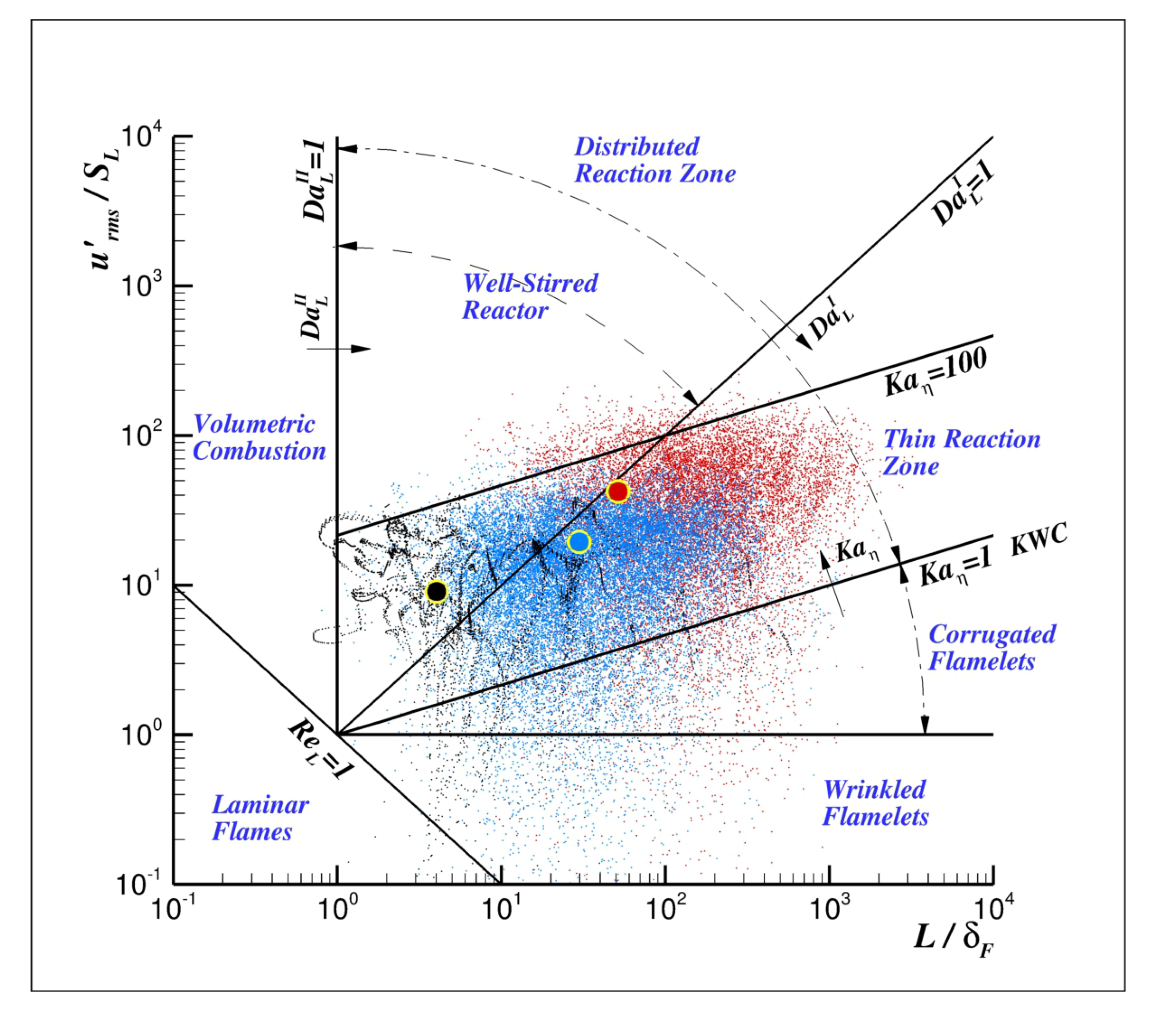
As a matter of fact, a real flame can experience several regimes depending on the local turbulent and chemical conditions. For example, Figure 1 reports on the standard combustion diagram the global states (the three big yellow marked points) of three CH 4 / H 2 / Air (equivalence ratio 0.7) premixed flames at 1, 10, and 40 bar, derived by DNS simulation data [23]. On the same diagram, combustion regimes associated with an instantaneous flowfield of the three flames are also reported; for these clouds of points, the quantities along the axis now have to be read as instantaneous quantities. Instantaneous local turbulent velocity and correlation length scales were calculated in the fresh mixture at the c = 0.1 value of the progress variable; the instantaneous local laminar flame speed was estimated according to the expression of Bougrine [24]; the instantaneous local flame thickness was calculated as the path length normal to the iso-c surfaces from 0.1 to 0.99. It is observed how the actual combustion regimes are spread around the global state point, covering different regions of the combustion map. It is also observed that the instantaneous distributions of the Prandtl number (not reported) exhibit P r 1 in every flames, and the distribution becomes wider by increasing pressure [23].
A central point in turbulent combustion modeling is the closure of the filtered chemical source term. Some models were designed to work in specific combustion regimes, e.g., Zimont [25,26,27] and Peters [21,28] developed turbulent flame speed ( S T ) models for a highly turbulent premixed combustion regime characterized by “flamelets” thickened by small-scale turbulent eddies penetrating into their preheating zone; Bray proposed how to estimate the domain of countergradient transport through his own characteristic number [29,30,31] and specific models for this mechanism mainly associated with weak, medium-scale turbulence were suggested [32,33]; Clavin introduced the effect of flame front stretch rate and curvature on flame speed for weakly perturbed laminar flames [34,35], later extended by Matalon to the weak turbulence (Markstein) regime [36]; Minamoto suggested a closure for the filtered reaction rate in LES of MILD combustion [37]. An important feature of the models adopted for such turbulent combustion closure would be their self-adaptation to the local combustion regime.
Upon the above literature review, it is clear that there exist different models specific for each combustion regime. A unified model covering all the regimes is currently missing. This motivates the present work whose final objectives are to build such a general framework, here called Localised Turbulent Scales Model (LTSM), and to develop a subgrid Large Eddy Simulation model for the chemical source terms, self-adapting to the local combustion regimes.
To reach its objectives, this work will be based on theoretical analysis of turbulent combustion and some well known results in specific combustion regimes. The article consists of two parts: in the first one, a methodology to identify the different combustion regimes locally exhibited by turbulent premixed flames will be presented (LTSM); in the second one, a subgrid scale model for the filtered chemical source terms will be provided and validated.

2. LTSM Theoretical Framework

The methodology adopted for the development of the theoretical framework of the Localised Turbulent Scales Model (LTSM) is presented here. The goal of the first part of the present article is the identification of premixed combustion regimes based on comparison of orders of magnitude (comparing the physical length and velocity scales involved in the process and reckoning on their possible interaction) and some assumptions. In particular, it is aimed at identifying combustion regimes by specifying their boundaries in terms of the turbulent Reynolds and Damköhler numbers and removing the unity Prandtl number assumption. In fact, actual local Prandtl number distributions in flames show values lower than one in ideal gas conditions; values greater than one are also possible in real gas conditions [38].
Identification of combustion regimes means to understand the spatial structure and morphology of the reacting flow resulting from the interaction of turbulent and chemical scales. Hence, the methodology adopted will consist of identifying when the flame can be considered locally laminar or turbulent, when combustion can be assumed to be volumetric or distributed, how eddies smaller or larger than the flame front can affect it, and then which eddies may survive to a flame front without being dissipated before combustion can take place at their scale, and among these ”survived” eddies which may wrinkle, thicken, or quench the flame front.

2.1. The Combustion Regime Identification Strategy

The analysis will take into account characteristic times at the generic eddy scale ; this eddy is assumed to belong to the Kolmogorov’s inertial range, η , Δ ( Δ being the local macro-scale and η the local dissipative scale) and thus it will have a characteristic velocity u = u Δ / Δ 1 / 3 . Characteristic times of different processes will be considered, such as the turbulent time τ t = / u , the viscous time τ ν = 2 / ν , the chemical time τ c h = δ L / S L = α / S L 2 = δ L 2 / α (the Mallard–Le Chatelier theory is adopted), α = κ / ( ρ C p ) being the thermal diffusivity, κ the thermal conductivity, ρ the density, and C p the specific heat at constant pressure. As a reminder, the laminar flame speed in the Mallard–Le Chatelier theory is estimated as follows:
S L α τ c h 1 / 2 ,
the laminar flame thickness as follows:
δ L α τ c h 1 / 2 ,
and that these two expressions imply the following equation:
δ L S L α = 1 .
The Prandtl number, the turbulent Reynolds, and Damköhler (first and second species) numbers will be defined from characteristic times and used to identify the boundaries of combustion regimes.
In the following sections, the scale * of the smallest “surviving” eddy (not dissipated by the flame front) will be firstly identified, and then checked if it may wrinkle the flame front, thus becoming a “wrinkling” eddy of scale w * . Then, it will be investigated if “survived” eddies of scale < δ L may thicken the flame front itself. Finally, comparing the newly defined length scales, combustion regimes will be naturally identified.

2.2. The Combustion Closure Strategy

The Favre filtered chemical source term in the energy and single species transport equations is modeled here as ω i ˜ γ * ω i * , γ * and ω i * being the local reacting volume fraction of the computational cell and the reaction rate of the i t h chemical species.
Let us consider a local control volume V Δ with characteristic dimension Δ = V Δ 1 / 3 and assume that it contains a flame front having an actual surface area A F and an actual thickness δ F and hence a reacting volume V F . It is possible to define the fraction γ * of the local reacting volume V F as follows:
γ * = V F V Δ A F δ F V Δ S T S L A L δ F V Δ S T S L Δ 2 δ F Δ 3 = S T S L δ F Δ .
This expression has been obtained with two main assumptions. The first is that, within a wrinkled flame front, the iso-surfaces of the progress variable are parallel [39]. The second assumption is that the ratio between the turbulent and the laminar flame surface areas scales as the ratio between the associated flame speeds and is expressed as follows:
A F A L A T A L S T S L .
Subgrid flame front physics is synthesized in this ratio: the subgrid flame may be laminar or turbulent, wrinkled or not, thickened by turbulence or not, depending on the local conditions of the flow. The γ * estimation becomes the problem of estimating the characteristics of the local flame front (turbulent flame speed, laminar flame speed and thickness, turbulent or laminar) from the filtered conditions of the flow and depending on the related local premixed combustion regime.
An extinction or flame stretch factor G e x t 1 , introduced in Section 4, is also included in Equation (4) to take into account flame quenching due to subgrid scales. Hence, the local reacting volume fraction is finally modeled as follows:
γ * = G e x t S T S L δ F Δ .

3. Vortices/Flame Front Interaction

This section aims to answer two fundamental questions related to the interaction problem between vortices and a flame front. What is the smallest eddy with a life-time longer than the characteristic chemical time? In addition, then, among the surviving scales, what is the smallest eddy able to locally wrinkle a flame front? Answering the first question allows for defining the range of scales that can interact with a flame front, and eventually enter into it and produce local flame thickening. Answering the second question allows instead for defining the smallest turbulent scales that apply the highest strain rate and curvature onto the flame front.

3.1. The Smallest Surviving Eddy

The interaction between a premixed flame front and eddies has been widely analyzed in the literature. Results clearly show that the dissipative Kolmogorov scales η cannot quench a flame front [22]. An estimate of the smallest turbulent scale that can affect a laminar flame front without being dissipated can be obtained by imposing that the turbulent scale Damköhler number of second species be greater than one, i.e.,
D a I I = τ ν τ c h = P r 1 δ L 2 1 ,
where τ ν = 2 / ν is the lifetime of the vortex of scale , τ c h = δ L / S L = δ L 2 / α is the chemical time, and P r = ν / α the Prandtl number.
It is stressed that the present analysis removes the P r = 1 assumption. Hence, the smallest surviving scale l * is estimated as follows:
* = P r 1 / 2 δ L = Δ D a Δ I R e Δ 1 / 2 = Δ D a Δ I I 1 / 2 ,
where R e Δ = u Δ Δ / ν is the turbulent Reynolds number defined in terms of the local length and velocity macro-scales, Δ and u Δ ; D a Δ I = Δ / u Δ τ c h is the turbulent Δ scale Damköhler number of the first species.
The smallest surviving scale * [ η , Δ ] for whatever Prandtl number if the following condition is met:
Δ * η R e Δ 1 D a Δ I R e Δ 1 / 2 D a Δ I R e Δ 1 ,
with * = Δ for D a Δ I = R e Δ 1 and * = η for D a Δ I = R e Δ 1 / 2 . It is observed that, for P r = 1 , it is always * δ L . Eddies * will not be dissipated by the flame front: for whatever Prandtl number, no eddies will survive for D a Δ I < R e Δ 1 , while the whole spectrum of eddies will for D a Δ I R e Δ 1 / 2 .
An important observation, of course valid in the present order of magnitude framework, is as follows:
* δ L P r 1 ,
and this means that, only for P r 1 , typical of ideal gas combustion, eddy-scales smaller than the flame thickness may survive and affect the flame itself, e.g., entering into it (although this has not been proved yet) and thickening it.
Another observation is that the Taylor micro-scale, λ g = Δ R e Δ 1 / 2 , could be used to estimate the local strain of the flow as u Δ / λ g in the eddy–flame interaction (flame strain modeling), according to the equation:
λ g * D a Δ I 1 .
This relation is always verified in the range of existence of * in (9) since 1 > R e Δ 1 (assuming the flow locally turbulent, i.e., R e Δ > 1 ).

3.2. The Smallest Wrinkling Eddy

Looking at the vortices/flame front interaction problem, some eddies will be destroyed by viscous dissipation before combustion can take place. The range of the surviving eddy-scales has been defined in Section 3.1. Among these scales, those smaller than the local flame front thickness may locally enter into it and thicken it, provided that u Δ S L , u Δ being the local r m s velocity fluctuation. The “surviving” condition is not sufficient for an eddy to locally wrinkle a flame front. Extending this concept to the generic scale l, only eddies with characteristic (tangential) velocity u S L will be able to locally wrinkle a flame front.
Given the smallest surviving eddy * = Δ D a Δ I R e Δ 1 / 2 within the inertial cascade, the smallest surviving and wrinkling eddy w * will be given by the following condition:
u * S L 1 u Δ S L * Δ 1 / 3 = P r 1 / 2 R e Δ D a Δ I 2 1 / 3 1 ,
Hence, the smallest surviving scale * becomes w * only if the following condition is met:
D a Δ I P r 3 / 4 R e Δ 1 / 2 u S L P r 1 / 6 Δ δ L 1 / 3 .
For higher Damköhler numbers, the smallest surviving scale * = Δ D a Δ I R e Δ 1 / 2 decreases but is unable to wrinkle the flame front; in this higher D a Δ I range, the smallest surviving and wrinkling scale becomes constant and equal to the minimum value w * m i n reached at D a Δ I = P r 3 / 4 R e Δ 1 / 2 . Substituting this maximum Damköhler number for the smallest surviving and wrinkling scale into Equation (8), the minimum w * is obtained as follows:
w * m i n = P r 3 / 8 η η .
Since inner cut-off scales are generally expressed in terms of the Karlovitz number, defined in Equation (26), the relation (14) can be rewritten as follows:
w * m i n / δ L = P r 3 / 8 K a t 1 / 2 .
This expression has the same K a t dependence as in [40], with P r 3 / 8 as the proportionality coefficient.
In summary, w * decreases as Δ D a Δ I R e Δ 1 / 2 by increasing D a Δ I up to D a Δ I = P r 3 / 4 R e Δ 1 / 2 . Then, w * maintains its minimum value P r 3 / 8 η for whatever D a Δ I P r 3 / 4 R e Δ 1 / 2 , implying that the highest local flame front curvature can be of the order w * 1 = P r 3 / 8 / η .
From what was found above and considering u * m i n = S L , the minimum scale Reynolds number for flame front wrinkling will be as follows:
R e w * m i n = S L * ν S L w * m i n ν = P r 1 / 2 1 .
It is observed that simple chemistry DNS calculations [22,40] showed the following equation:
w * m i n δ L = 0.2 + 5.5 ε δ L S L 3 1 / 6 R e w * m i n 5 . 5 3 / 2 D a I 1 / 2 P r 1 ,
with ε = u 3 / . Experimental work [41,42] instead showed the following equation:
u w * m i n S L = 2.5 w * m i n δ L 1 R e w * m i n 2.5 P r 1 .
Large differences are expected between experiments, simple chemistry DNS calculations, and theoretical results. However, the trends of these three approaches are qualitatively well reproduced, looking at the R e w * m i n = f P r dependence.

3.3. The T urbulence- T hickened R egime

In Section 3.1, it was shown that some scales smaller than the flame thickness may not be dissipated. These scales may affect the flame front itself thickening it. In particular, it was theorized that eddies * δ L exist only for P r 1 and hence the T urbulence- T hickened R egime cannot be experienced when P r > 1 .
In the literature, there is a well known model for the turbulence-thickened regime: it is the Zimont’s model [25,26,27]. According to this model, the chemical time does not change through the whole thickening process: considering the flame front composed of a reaction layer, δ r , and a thermal (preheating) layer, δ t l , a constant τ c h implies that δ r is not affected by the flow, while δ t l may be thickened by the survived eddies.
The thickening process can be modeled via a turbulent thermal diffusivity α * u * t k * , u * being the characteristic velocity of the scale t k * u * τ c h that is the survived and thickening turbulent scale obtained via Equation (7) with a turbulent viscosity ν * u * t k * . With these assumptions, the thickened flame front δ F * can be estimated as follows:
δ F * α * τ c h 1 / 2 u * t k * τ c h 1 / 2 u * τ c h Δ D a Δ I 3 / 2 ,
having obtained u * via the turbulence energy cascade, u * u Δ ( t k * / Δ ) 1 / 3 u Δ D a Δ I 1 / 2 . It is observed that t k * has to be larger than or equal to * given by Equation (8) and, in particular, it comes out that t k * δ F * . The same result for δ F * is obtained, as in Zimont’s model [25,27], by assuming α * u * t k * u * δ F * , i.e., that the smallest surviving scale is of the order of the thickened flame front.
From Equation (19), the laminar thickened flame speed is as follows:
S L * α * τ c h 1 / 2 u * δ F * τ c h 1 / 2 u Δ D a Δ I 1 / 2 u * .
Assuming S T / S L A T / A L and assuming the ratio between the turbulent and laminar flame surface areas, A T / A L D a Δ I 3 / 4 [25,27], the turbulent thickened flame speed can be scaled as
S T Z A Z S L * A T A L A Z S L * D a Δ I 3 / 4 A Z u Δ D a Δ I 1 / 4 ,
A Z = 0.5 being an empirical constant [26,43]. Assuming that the chemical time is unchanged, i.e., δ F T / S T Z = τ c h , the thickness of the turbulence-thickened flame front is as follows:
δ F T Z S T Z τ c h A Z Δ D a Δ I 3 / 4 .
In terms of Prandtl and turbulent Reynolds numbers, S T / S L Z becomes the following equation:
S T S L Z A Z P r R e Δ 1 / 2 D a Δ I 1 / 4 .
Imposing the conditions reported in Table 1, the T u r b u l e n c e - T h i c k e n e d flame R e g i m e validity ranges are obtained in terms of the local Damköhler number, D a Δ I . It is observed that the Zimont constant A Z was not considered in this analysis, specifically in conditions 9–12.
In particular, the constraint number 12 in Table 1 requires that the volume fraction γ * in Equation (4) be less than one. Having adopted a model for the reacting volume fraction, subgrid flame front wrinkling and curvature effects are synthesized in the quantity γ * . Considering the Zimont’s model [25,26,27], the expression for the local reacting volume fraction γ * in the turbulent thickened flame regime becomes as follows:
γ * = S T S L δ F Δ = S T S L Z δ F * Δ ,
with δ F * and S T / S L Z given by Equations (19) and (21), respectively.
Imposing the constraints in Table 1, the T u r b u l e n c e - T h i c k e n e d flame R e g i m e validity ranges are obtained in terms of the local Damköhler number, D a Δ I , according to the following equation:
P r 1 / 2 R e Δ 1 / 2 D a Δ I P r 2 / 7 R e Δ 2 / 7 f o r 1 P r R e Δ 1 .

4. The Extinction Factor

The wrinkling scales, and in particular the smallest one w * that imposes the highest strain onto the flame front, can stretch a flame front up to local quenching, thus becoming quenching scales.
To have local quenching, the thickness of the flame front has to be smaller than the local integral macroscale. Hence, if δ L Δ ( V o l u m e t r i c R e g i m e ) no quenching due to eddy flame stretching is possible: no q * exist for D a Δ I P r 1 R e Δ 1 (see Section 5). This is a first boundary of the quenching region in the combustion diagram: this boundary seems to be confirmed by the quenching model described below that compares well with experimental and DNS numerical data.
The Karlovitz number is related to the effect of aerodynamic stretching on the flame front and is defined as the ratio between the chemical time and the stretching time and is presented as follows:
K a t = τ c h τ s t K a η t = δ L / S L η / u η = P r δ L η 2 δ L η 2 .
By defining the Karlovitz number as in Equation (26), it is assumed that the η scales are the most important or effective in stretching a flame. The smallest wrinkling eddy applies the highest strain on the flame front, hence it may be the most effective to produce quenching. Considering that the Karlovitz number defined in Equation (26) can also be expressed as K a η = R e Δ 1 / 2 / D a Δ I , the existence condition for the smallest wrinkling scale in Equation (13) can be rewritten as K a η P r 3 / 4 that is only a bit higher than the Klimov–Williams criterion.
This existence condition of the smallest wrinkling eddy is a necessary but not sufficient condition for quenching. In fact, Peters [6] observed that actual flames resist strain more than predicted by the Klimov–Williams (Karlovitz) criterion.
In the literature, there are some models that provide an extinction or stretch factor G e x t 1 that can be effectively used to “damp” locally the reaction rate, thus mimicking the effect of subgrid flame stretching.
An extinction or stretch factor G e x t was firstly introduced by Bray [44] and then adopted in models [26,27,
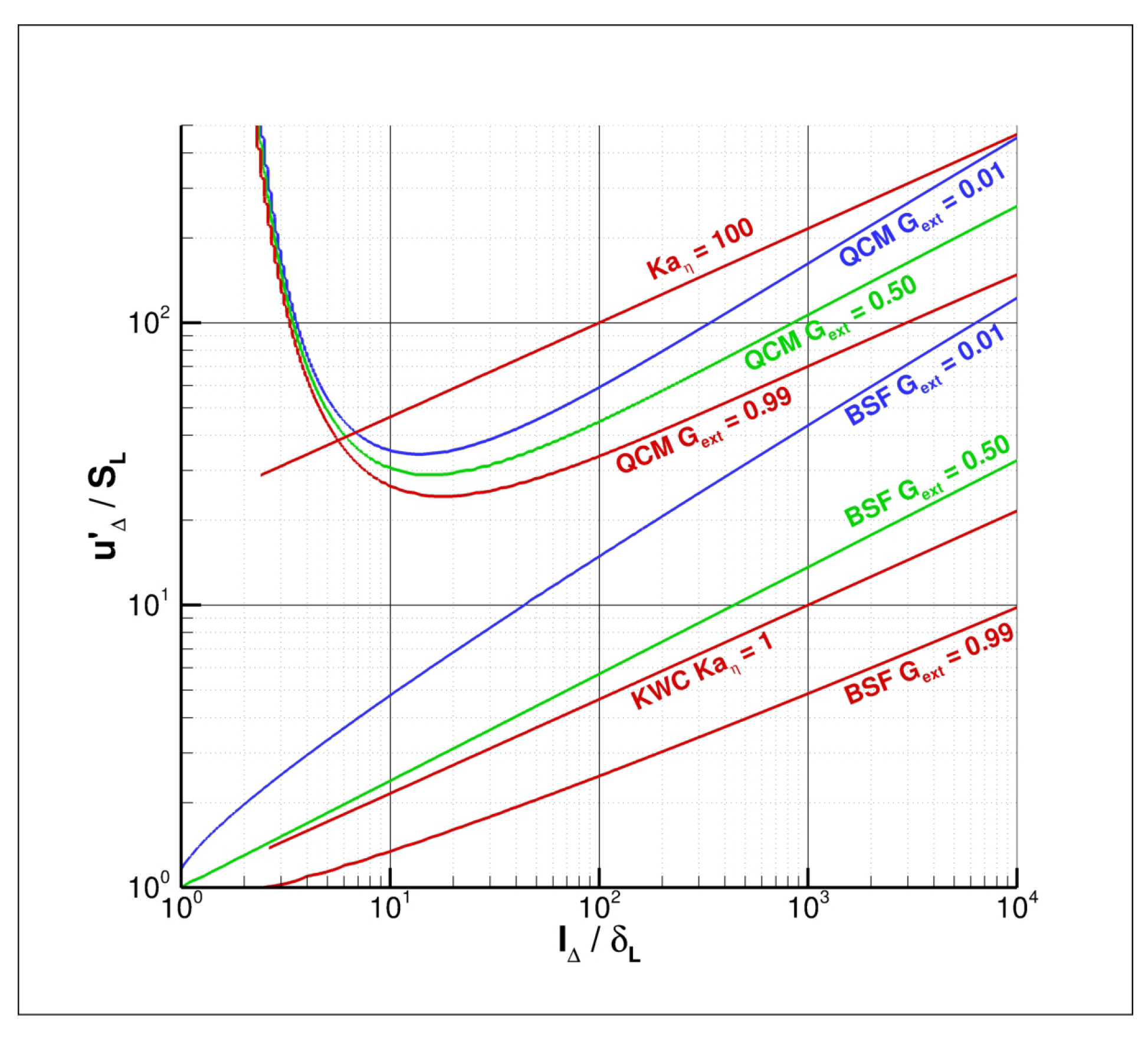
45]. However, quenching predictions based on the Bray’s stretch factor (BSF curves in Figure 2) or on the Klimov–Williams criterion discussed in Section 1 (KWC line) both do not agree with those found from both experiments and direct numerical simulations that provide, in fact, similar trends [22,42,46].
A model that can be more effectively used to predict quenching is the so-called quenching cascade model [46] that compares quite well with experimental and direct numerical simulation data on quenching ([42], pp. 212–214). The main assumptions at the base of the model are:
1
However strong the vortex strain may be, the time required to quench the flame is the same and it is given by τ c h = δ F / S L ;
2
Only eddies with large characteristic velocity u (at least S L ) are able to quench the flame;
3
If the mean eddy life-time is smaller than the chemical time τ c h , such eddies cannot quench the flame;
4
A temporal sequence of approximately τ c h / τ consecutive eddies of size with large u must exist to induce actual quenching;
5
The mean eddy time-scale τ is estimated considering a multifractal description of turbulence with intermittency;
6
A discrete set of scales is recursively generated.
With these assumptions, the quenching cascade model estimates the total fraction of flame surface undergoing quenching during a time τ c h .
Three G e x t isolines of the quenching cascade model are shown in Figure 2, where they are compared with the associated isolines of Bray’s stretch factor, the Klimov–Williams criterion K a η = 1 and the K a η = 100 line suggested by Peters. In particular, the four red lines should be compared. Above them, extinction is predicted at different levels by these models. Since the extinction region predicted by the quenching cascade model has been validated with experimental data [22,42,46], it is assumed as a reference model: hence, high velocity fluctuations are required to produce localized flame quenching. While the Bray’s stretch factor and the Klimov–Williams criterion underestimate extinction, the Peters’ criterion seems to overpredict the flames’ capability of resisting strain.

5. Premixed Combustion Regimes

Thinking about the interaction between a flame front and turbulent eddies, it is possible to identify different combustion regimes through the comparison of the previously defined length scales ( Δ , η , * , w * , t k * , δ L ) involved in the process.
At first, the local laminar flame front δ L , the turbulent macro-scale Δ , and the turbulent dissipative scale η are compared. The regime associated with δ L Δ is named V o l u m e t r i c R e g i m e , V R . The regime associated with δ L < η is named W r i n k l e d R e g i m e , W R . These two combustion regimes are experienced, respectively, for low and high Damköhler numbers of first species, as shown in Table 2.
Between V R and W R , there is a more complex regime consisting of other subregimes. In fact, when Δ > δ L η , some eddies may not be dissipated by the flame front, some may corrugate it, and in particular conditions of the Prandtl number, some may even thicken it: the role played by these scales is shown in Figure 3. The subregime characterized by w * > * is here called C o r r u g a t e d R e g i m e , C R . The subregime characterized by w * = * is named T h i c k e n e d R e g i m e , T R . As discussed in Section 3.3, in certain ranges of the Prandtl number, the flame front may be even thickened by some eddies: this subregime is here named T u r b u l e n c e T h i c k e n e d R e g i m e , TT R . The intermediate combustion regime in Table 2 is named TTC R (since it includes both the TT R and C R regimes), and it nearly corresponds to the pocket flames region defined by Barrère [2]: the region with D a 1 corresponds to the W ell- S tirred R eactor; the region including the T h i c k e n e d and the T u r b u l e n c e - T h i c k e n e d regimes corresponds to the Distributed Reaction Zone.
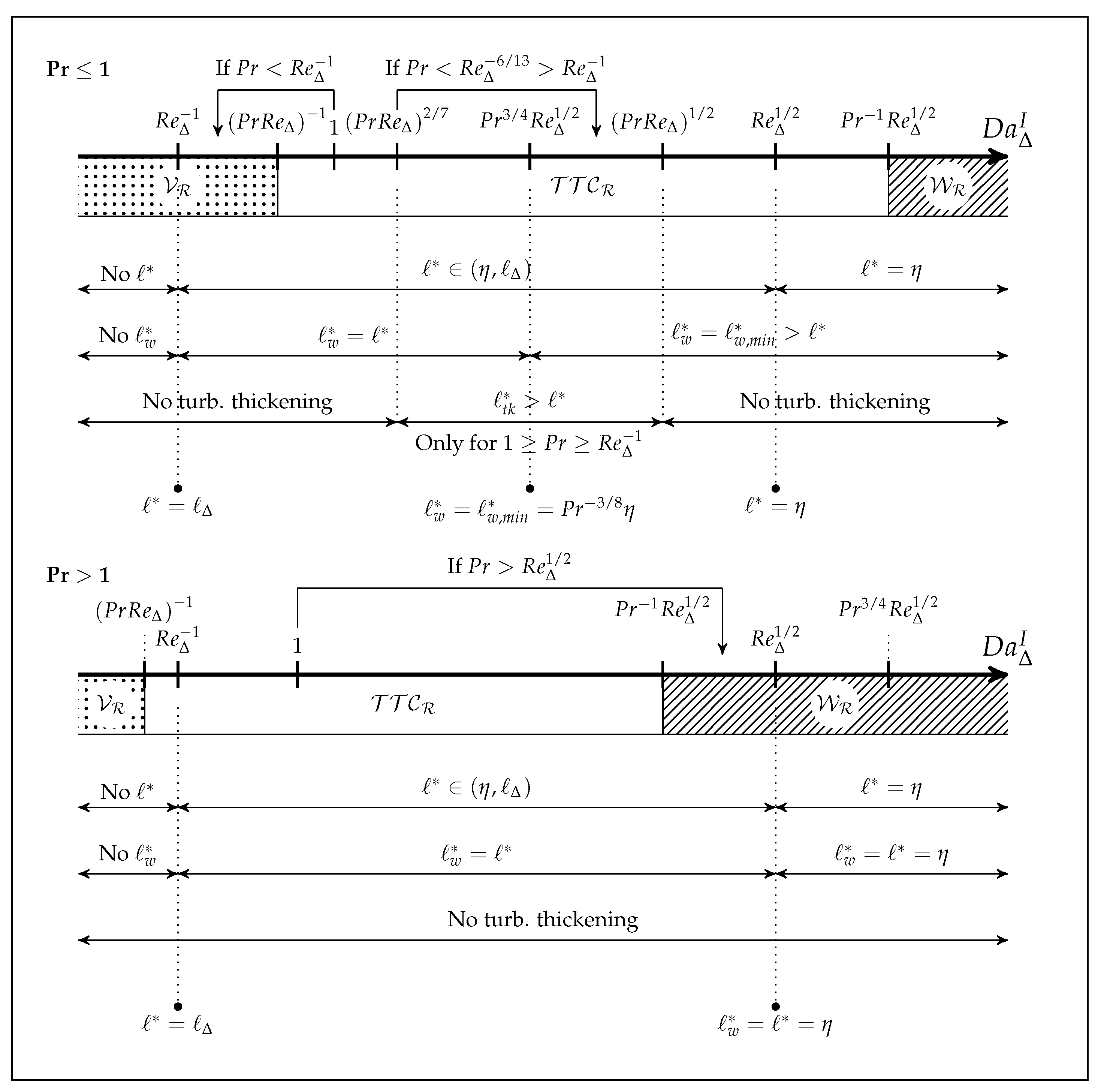
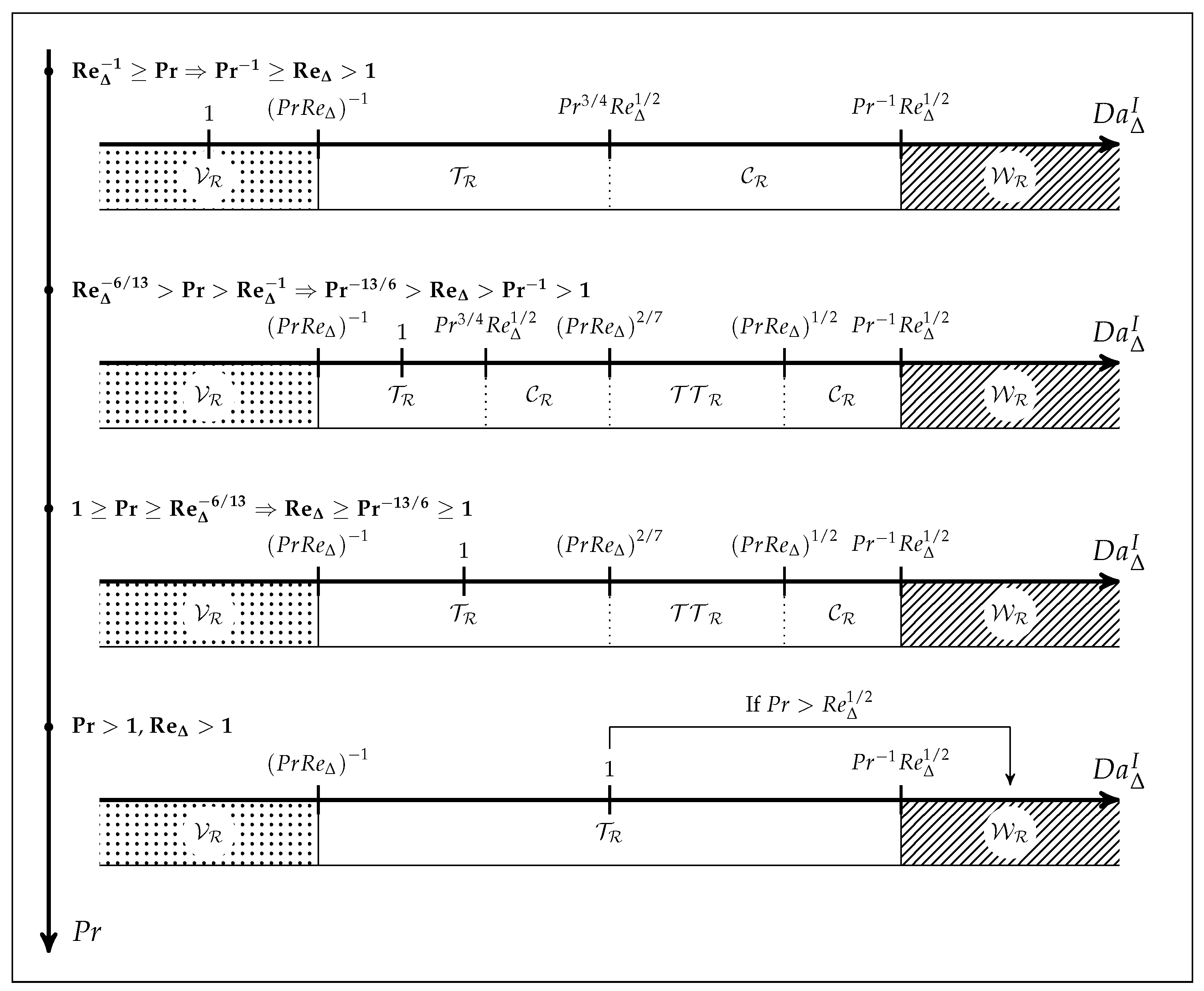
The premixed combustion regimes described in Table 2 are described with more details in Figure 4. Depending on the local Prandtl number, there can be four possible conditions: three of them relating to P r 1 and only one to P r > 1 .

The Most Probable Condition for P r 1

Considering that common gases have P r [ 0.2 , 1 ] and that a sufficiently high Reynolds number is required (i.e., Δ / η 10 at least) to experience turbulence/combustion interaction, among the three conditions characterized by P r 1 , the third one is the most physical. In fact, in the first case, the Prandtl number would be very low even for high Reynolds; in the second case, the Prandtl number would be too low for gaseous combustion at sufficiently high Reynolds numbers. For this reason, and since the condition with P r > 1 appears “simpler”, the condition 1 P r R e Δ 6 / 13 will be analyzed in more detail in the following. The condition 1 P r R e Δ 6 / 13 implies that turbulence/combustion interaction will be assumed to happen for R e Δ P r 13 / 6 , being P r 1 . For R e Δ P r 13 / 6 , the flame will be considered locally laminar.
The boundary lines of each regimes are reported in Table 3. Such information is used to build the LTSM combustion diagram in Figure 5 for 1 P r R e Δ 6 / 13 both in the u Δ / S L v s . Δ / δ L and D a Δ I v s . P r R e Δ logarithmic planes. As a reminder, in the LTSM framework, these diagrams refer to local quantities and not to global ones as in the standard combustion diagram (in fact, the turbulent scales considered are u Δ and Δ instead of u r m s and L).
In the u Δ / S L v s . Δ / δ L plane, there are two boundaries that can change depending on the local Prandtl number: the first is the laminar region boundary, R e Δ = P r 13 / 6 , that corresponds to the R e Δ = 1 line of the standard combustion diagram but shifted upwards depending on the P r < 1 value; the second is the lower boundary of the C o r r u g a t e d R e g i m e (that is also the top boundary of the W r i n k l e d R e g i m e ), that shifts downwards depending on the P r < 1 value (the C R regime disappears for P r = 1 ). The lower boundary of the T u r b u l e n c e T h i c k e n e d R e g i m e (that is also the upper boundary of the C o r r u g a t e d R e g i m e ) is the K a η t = 1 line with P r = 1 (that is the quenching line in the Klimov–Williams criterion).
Figure 6 shows the main scales of turbulence and combustion and the regimes for 1 P r R e Δ 6 / 13 , i.e., for R e Δ P r 13 / 6 , with P r 1 . It is observed that, in this range of Prandtl number, the conditions * = λ g and w * = w , m i n * reported in the top frame of Figure 6 cannot be reached since R e Δ 1 < R e Δ 6 / 13 . Focusing on the eddy length scales and considering that the flame front destroys eddies smaller than * , it is observed that the turbulent energy cascade is not fully active everywhere: where * > η the energy cascade stops at scale * .

6. Modeling the Reacting Volume Fraction

In the Large Eddy Simulation framework, the local turbulent macro-scale Δ will be assumed equal to the characteristic size of the computational cell (filter size), estimated through its volume, i.e., Δ = V Δ 1 / 3 ; its associated velocity, u Δ , will be assumed equal to the subgrid velocity derived through the specific eddy viscosity model adopted in the simulation. In Section 2.2, the strategy adopted for turbulent combustion closure was introduced: the Favre filtered chemical source term in the energy and single species transport equations is modeled as ω i ˜ γ * ω i * , where the local reacting volume fraction of the computational cell is modeled as in Equation (6).
In Equation (6), the laminar flame speed is estimated as S L α / τ c h 1 / 2 . The turbulent flame speed and the flame front thickness will be modeled depending on the combustion regimes. In particular, the laminar flame thickness will be estimated as δ L α τ c h 1 / 2 but not in the T u r b u l e n c e - T h i c k e n e d R e g i m e where its thickened counterpart defined in Equation (19) will be assumed. The local filtered chemical time required to estimate laminar quantities can be calculated as τ c h = ρ C p T / Δ H R , where Δ H R = i = 1 N s H i ω i ˙ is the heat of reaction, N s being the number of chemical species, H i = h f i 0 ( T r ) + Δ h s i ( T ) the enthalpy of the i-th chemical species, h f i 0 ( T r ) its formation enthalpy at the reference temperature T r = 298.15 K , Δ h s i = T r T C p i ( T ) d T its sensible enthalpy, and ω i ˙ its reaction rate.
In conclusion, the local P r , R e Δ , D a Δ I are first calculated. Based on these characteristic numbers, subgrid turbulent combustion is taken into account by modeling γ * by means of the expressions summarized in Table 4. These expressions guarantee γ * 1 ; the identity Δ Δ was assumed in deriving their non-dimensional number dependence. It is observed that the Zimont expression for S T has been assumed not only in the T u r b u l e n c e - T h i c k e n e d R e g i m e but also in the C o r r u g a t e d R e g i m e , due to the lack of reliable experimental data [43] and the superiority of the Zimont model with respect to other models [43]. In the W r i n k l e d R e g i m e , subgrid hydrodynamic effects and Lewis number effects on S T have been neglected for the time being. However, it is observed that this regime appears to be of minor importance in industrial applications [43]. Work is currently going on by the present authors to define, in this low strain regime (Markstein regime), a X factor taking into account thermo-diffusive effects (induced by reactants’ Lewis number) that increase or decrease the turbulent flame speed and flame wrinkling: S T / S L = 1 X , with X > 0 or X < 0 depending on local curvature, strain, and Markstein number sign.

7. Model Validation

The Localised Turbulent Scale Model is validated here against data coming from a Direct Numerical Simulation performed by these authors [47]. In particular, the time average and rms fluctuation of some quantities resulted from the LES simulation were compared with their DNS counterpart.

7.1. The Test Case

The test case consists of an unconfined and atmospheric Bunsen flame developing along the streamwise direction (z). This premixed flame is produced by three adjacent rectangular slot burners whose size is undefined in the spanwise direction (x) (due to the periodic boundary conditions imposed in the simulation) and that are separated along the transversal direction (y) by means of two 0.17 mm thick walls. The central slot burner injects a fresh mixture of methane, hydrogen, and air, while the two side burners inject hot combustion products of the same central mixture.
The reactant mixture, with an equivalence ratio Φ = 0.7 and with 0.2 mole fraction of hydrogen, is injected from the central slot with a bulk velocity of 100 m s 1 and at 600 K . The velocity of the coflow stream is 25 m s 1 . The central jet Reynolds number is 2253, based on the width of the jet, 1.2 mm , its bulk velocity, and the kinematic viscosity 5.327 · 10 5 m 2 s 1 . Homogeneous isotropic turbulence is forced at the inlet. Such turbulence is artificially produced by means of a synthetic turbulence generator implemented from [48]. In particular, the spatial correlation length scales and velocity fluctuations provided as input to this generator are: L z z = 0.8 mm , L x x = L y y = L z z / 2 = 0.4 mm , u z = u x = u y = 12 m s 1 with no shear stresses (the Reynolds stress tensor is diagonal) [49].

7.2. The Numerical Set-Up

The computational domain is three-dimensional with 61 nodes in the spanwise direction (x), extending from −1.5 to 1.5 mm , and along which periodic boundary conditions are forced. The computational domain has four zones: a central injection zone extending from 4 mm to 0 in the streamwise direction (z) with a width (along y) of 1.2 mm and with 60 × 35 nodes ( z y ); two surrounding zones extending from 0.4 mm to 0 in the streamwise direction and from the central slot external wall (wall thickness 0.17 mm ) up to 18 mm outward in the transversal direction (y) with 8 × 89 nodes ( z y ); a main mixing and reacting zone downstream of the injection extending from 0 to 24 mm in the streamwise direction and from 18 mm to 18 mm in the transversal direction with 241 × 221 nodes ( z y ). The whole computational domain has 56,785 × 61 = 3,463,885 nodes.
Since the LES results are going to be compared against DNS numerical data, it is useful to quantify how much the LES computational grid is coarser than the DNS grid. Here, we simply report the main quantities of the two grids: the Δ y L E S / Δ y D N S spacing ratio is in the range 1.42–6.25, and the Δ z L E S / Δ z D N S is in the range 3.14–8.21, with the higher values reached in the flame front region; the ratio between the aspect ratios, ( Δ y L E S / Δ z L E S ) / ( Δ y D N S / Δ z D N S ) , is in the range of 0.17–2.00.
The simulation was performed using the same in-house HeaRT code previously used for the DNS, which solves the fully compressible reactive Navier–Stokes equations in their conservative formulation. The fully explicit third-order accurate TVD low-storage Runge–Kutta scheme of Shu and Osher [50] is used for temporal integration. A staggered formulation of the transported quantities is adopted for the spatial integration: a second-order centered scheme is used for all diffusive fluxes and momentum convective terms, while scalar convective terms are modeled through the AUSM method coupled to a third-order QUICK interpolation. No artificial damping or filtering was necessary for ensuring a stable solution.
The ideal gas equation of state is assumed. The same models adopted to estimate molecular transport properties in the DNS calculations are here adopted. The Hirschfelder and Curtiss [51] approximate formula is adopted to model molecular transport in a multicomponent mixture, taking into account preferential diffusion effects. The Soret thermo-diffusive effect is also considered. Molecular transport properties for individual species, except their binary mass diffusivities, are accurately calculated through kinetic theory by using a priori the software library provided by A. Ern (EGlib) [52,53]. The calculated values are stored in a look-up table from 200 to 5000 K every 100 K. Values at intermediate temperatures are calculated at run-time by linear interpolation and then used to derive mixture-average properties through the Wilke’s formula with Bird’s correction for viscosity ([54], pp. 23–29) and Mathur’s expression for thermal conductivity ([54], pp. 274–278). Binary mass diffusion coefficients are calculated by means of kinetic theory expressions ([54], pp. 525–528) at run-time. Thermo-diffusion coefficients required to model the Soret effect are calculated at run-time by using the EGlib routines. The chemical mechanism adopted is a skeletal mechanism having 17 transported species and 58 reactions; in particular, the transported species are: CH 4 , H 2 , O 2 , N 2 , OH , O , H , HO 2 , H 2 O 2 , CH 3 , CH 2 , CH , CH 2 O , HCO , CO , CO 2 , H 2 O [55].
The walls are assumed viscous and adiabatic. Velocity, temperature, and mass fractions are fixed at the inlet, with turbulent velocity fluctuations artificially generated [48]. Periodic boundary conditions are applied in the spanwise direction, while improved partially non-reflecting outflow boundary conditions are imposed at the other open boundaries of the computational domain [56,57]. The subgrid scale model adopted for the turbulence closure is the dynamic Smagorinsky model [58]. This is used not only to calculate the eddy viscosity μ t , but also the instantaneous and local subgrid velocity fluctuation required in the LTSM model, i.e., u Δ = μ t / C S ρ Δ where C S is the Smagorinsky constant calculated dynamically.

7.3. The Results

The actual velocity fluctuation at the end of the injection channel is u 12 m s 1 , and the turbulent length scale is L t 1.05 mm . Using these quantities and the kinematic viscosity of the fresh mixture, the central jet turbulent Reynolds number is 236, and the Kolmogorov length scale is η 17.42 μ m. The adiabatic flame temperature is 2072 K . The laminar flame speed and flame front thickness (estimated from kinetics simulations including the Soret effect) at these conditions are S L = 1.01 m s 1 and δ F = 0.378 mm , respectively. Hence, u r m s / S L = 11.88 and L t / δ F = 2.78 ; K a η = 471 , D a L t I = 0.24 , thus ideally locating this flame into the broken reaction regime of the standard combustion diagram, well above the Peter’s boundary K a η = 100 of the thin reaction zone and where turbulence is expected to strongly influence premixed flame structure.
However, such a conclusion based on this commonly accepted procedure is wrong. In fact, the distribution of reacting cells reported for an instantaneous DNS flowfield in Figure 7. To build this diagram, a progress variable was defined as the normalized sum of CO 2 , CO , H 2 O , and H 2 mass fractions. Then, the iso-surface c = 0.1 (in the fresh mixture) was selected; on this surface, the auto-correlation length scales Δ and rms velocity fluctuations u Δ were calculated: these quantities characterize the local eddies interacting with the local flame front. On the same surface, the local laminar flame speed S L was also estimated through the method developed in [24]; the local flame front thickness δ L was estimated as the curvilinear length of the curvilinear segment normal to the iso-c surfaces starting from c = 0.1 and ending at c = 0.99 . shows that the flame experiences all the combustion regimes depicted within the LTSM framework. Most of the flame belongs to the thin reaction zone and only the reacting regions close to the flame tip ( z > 1.5 cm ) enter the quenching region with an increased probability of localized extinctions for the farthest regions from the inlet.
The comparison between LES and DNS data are very good in terms of averaged data, and good in terms of rms fluctuations. In fact, the average streamwise velocity and temperature flowfields look very similar. For brevity reasons, only a brief analysis comparing transversal and axial distributions of main quantities is provided in the following; more results are provided in the Supplementary Materials.
In the LES case, the temporal statistics were calculated by means of 22,033 transversal planes, sampled in 4.4 ms . Since the DNS is more computationally expensive, it was run for an admissible CPU time collecting 152 time-samples of the complete three-dimensional flowfields in 1.73 ms ; to enhance the convergence of the otherwise poor temporal statistics, every single plane (140) in the spanwise direction of the 152 3D-samples was assumed as an independent event, thus increasing the number of samples to 21,280. Inspecting contour maps of rms velocity fluctuations (not show here) built according to this strategy, it was observed that the profiles of the DNS data exhibit less symmetry with respect to the central jet axis than LES data, and this was more visible moving downstream. This was attributed to the lack of a fully converged statistics of the DNS rms data: since the tip of the flame is the most unstable region of the flow, exhibiting strong transversal oscillations and localized extinctions, more samples would be required. Hence, since the flow is topologically symmetric with respect to the central axis of the jet, the two transversal half-planes were considered as independent events in both LES and DNS, thus doubling the number of samples. However, these statistics are not still fully converged for the whole transversal plane, especially for rms fluctuations far downstream from injection. This is clear comparing the LES and DNS average and rms fluctuation of the streamwise velocity and temperature distributions along the central jet axis (see Supplementary Materials). This suggests to limit the comparison of transversal profiles up to 6 h, i.e., 7.50 mm , above the injection: the heights 2 h and 5 h are reported in the paper, while the others are available in the Supplementary Materials.
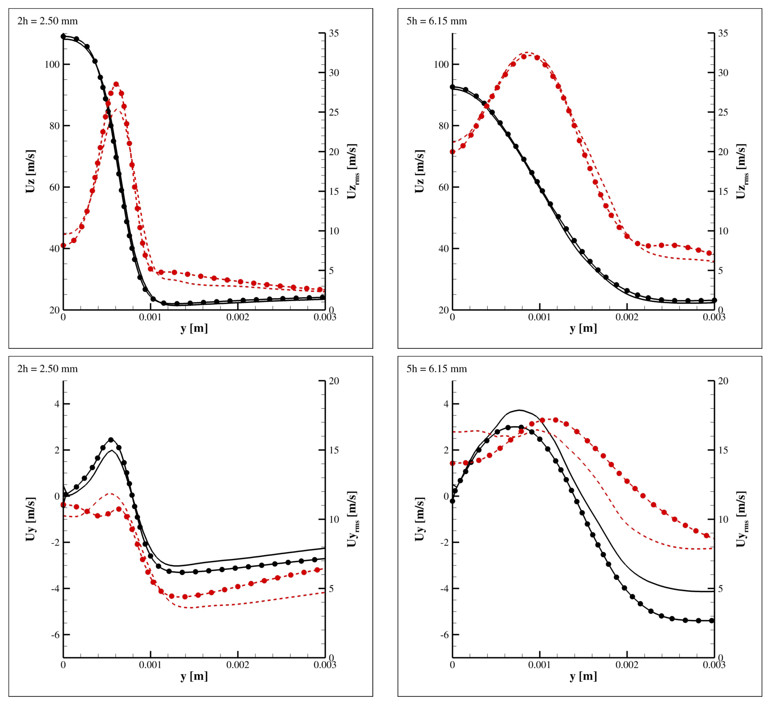
Looking at streamwise velocity profiles in Figure 8 (top), it is observed that the average turbulent flat profiles quickly evolves into the one characteristic of a free jet, with peak velocity fluctuation located in the two shear-layers. The agreement between LES and DNS average data are very good, while that of rms fluctuations is good, showing lower LES peaks in the shear-layers up to 4 h and an LES profile translated towards a bit higher values at 6 h. Similar comments can be drawn for the transversal velocity profiles in Figure 8 (bottom) that, in general, exhibit a worse agreement.
Looking at temperature profiles in Figure 9 (top), it is observed that the agreement between averaged LES and DNS data are also very good, with a maximum error of ∼50 K over temperatures of the order of 1000 K along the central axis in the most downstream sections. The location of rms temperature peaks is well predicted, but the amplitude of the LES peaks exhibits an error of ∼70 K over temperatures of the order of 600 K in the middle sections, 3 h and 4 h. Along the central axis, the rms agreement deteriorates starting from the 4 h section and increases moving more downstream.
Mass fraction of main species are then compared in terms of their time averages at the same locations in Figure 9 (bottom), showing a good agreement too. It is observed that the H 2 O profiles are not reported since they are very similar to the CO 2 profiles, both in shape and value. The worst agreement is achieved for the OH radical species.
It is observed that both temperature and velocity (especially the transversal one) profiles at the first two heights reveal that the dynamics of the flow downstream of the two walls separating the central jet from the side hot jets is not well captured by the LES simulation. This disagreement can be attributed to the poor spatial resolution of the LES grid to describe the thin wake regions of the two separating walls. Despite this, it is concluded that the transversal spreading of the flame is well reproduced at different heights from the injection, both in terms of velocity and temperature distributions. This implies that the coupling between the adopted turbulence and combustion models, i.e., the dynamic Smagorinsky and LTSM models, is effective in capturing the correct behavior of the present jet flame.

8. Discussion

This work provided a brief overview on how combustion regimes are introduced in standard and spectral combustion diagrams. Evidence that different regimes are experienced locally by the same turbulent flame has been given, reporting actual combustion diagrams for different DNS flame simulations. The actual combustion diagrams derived by DNS data are built on local quantities: auto-correlation length scales, rms velocity fluctuations, laminar flame speed, and flame front thickness. In particular, for one of these DNS cases, it is shown that the actual turbulent flame not only experiences several combustion regimes, but also that the global nominal combustion regime predicted according to the common methodology based on the global Karlovitz and Damköhler numbers is completely wrong.
Hence, a new perspective to look at combustion diagrams has been suggested. The analysis adopted consists of the identification of the main scales involved in turbulent combustion physics, in defining their role and their possible interaction. The result of this reckoning is a model describing combustion regimes in terms of turbulence and combustion scale interaction: this theoretical framework has been named LTSM, Localized Turbulence Scales Model. Adopting such a model as a subgrid scale model for Large Eddy Simulation implies assuming the local LES filter size as the local macro-scale Δ , and the subgrid velocity fluctuation derived by the specific eddy viscosity model adopted as its associated local velocity scale.
Based on this framework, a closure for the filtered chemical source term in the context of Large Eddy Simulation has been suggested. The turbulent combustion subgrid scale model consists of modeling the local reacting volume fraction γ * as in the Eddy Dissipation Concept, but the model depends on the combustion regime locally experienced. More specifically, γ * depends on the turbulent and laminar flame speeds ratio, and on the flame thickness; in terms of non-dimensional numbers, it depends on the Prandtl, Reynolds, and first species Damköhler numbers.
Finally, the suggested subgrid model has been validated by comparing LES and DNS data related to an unconfined and atmospheric slot burner flame with two adjacent hot coflows. Average, rms velocity and temperature fluctuations, and average mass fractions ( CH 4 , H 2 , CO 2 , CO , OH ) compare very well against DNS data. This, coupled with the interesting LES/DNS grid ratios adopted, confirms the goodness of the suggested subgrid model for the filtered chemical source term.

9. Conclusions

This work is an attempt to respond to the lack of a unified subgrid turbulent combustion model for Large Eddy Simulation, as shown from the literature review reported in Section 1, and this represents the novelty and value of the contribution of the paper. The Localised Turbulent Scales Model (LTSM) with its closure of filtered chemical source terms is the suggested model, able to self-adapt to the local combustion regimes taking into account the different conditions of the flow (turbulence, thermodynamics, composition, diffusive transport, acoustics). Although its reported validation against DNS data reveals it as a promising subgrid model, further comparison against experimental data and other combustion models would contribute to its robustness, applicability, and reliability; this will be the objective of future works.

Supplementary Materials

The following are available online at https://www.mdpi.com/article/10.3390/en14164934/s1: Section S1: History of Combustion Diagrams, Section S1.1: The Standard Combustion Diagram, Section S1.2: The Spectral Combustion Diagram, Section S2: Other Results for the Model Validation, Figure S1: Combustion regime identification on the standard and spectral combustion diagrams, Figure S2: Average streamwise velocity and temperature fields, Figure S3: Average and rms fluctuation of streamwise velocity and temperature along the central jet axis, Figure S4: Transversal average and rms streamwise velocity profiles at several heights, Figure S5: Transversal average and rms transversal velocity profiles at several heights, Figure S6: Transversal average and rms temperature profiles at several heights, Figure S7: Transversal average mass fraction profiles of several species at several heights.

Author Contributions

Conceptualization, E.G.; methodology, E.G.; software, E.G. and D.C.; validation, E.G. and D.C.; formal analysis, E.G. and D.C.; investigation, E.G. and D.C.; resources, E.G. and D.C.; data curation, E.G. and D.C.; writing—original draft preparation, E.G. and D.C.; writing—review and editing, E.G. and D.C.; visualization, E.G. and D.C.; supervision, E.G.; project administration, E.G; funding acquisition, E.G. All authors have read and agreed to the published version of the manuscript.

Funding

This research was funded by the Italian Ministry of Economic Development, Electric System Research project “Theme 1.2”. The APC was funded by the same project.

Data Availability Statement

Data supporting reported results can be asked to the authors.

Acknowledgments

The computing resources and the related technical support used for this work have been provided by CRESCO/ENEAGRID High Performance Computing infrastructure and its staff [59]. CRESCO/ENEAGRID High Performance Computing infrastructure is funded by ENEA, the Italian National Agency for New Technologies, Energy and Sustainable Economic Development and by Italian and European research programs (see http://www.cresco.enea.it/english, 11 August 2021).

Conflicts of Interest

The authors declare no conflict of interest. The funders had no role in the design of the study; in the collection, analyses, or interpretation of data; in the writing of the manuscript, or in the decision to publish the results.

References

  1. Williams, F.A. Combustion Theory, 2nd ed.; Addison-Wesley Publishing Company: Boston, MA, USA, 1985. [Google Scholar]
  2. Barrere, M. Modeles de Combustion. Rev. Gen. Therm. 1974, 148, 295. [Google Scholar]
  3. Bray, K.N.C. Turbulent Flows with Premixed Reactants in Turbulent Reacting Flows. In Topics in Applied Physics; Libby, P.A., Williams, F.A., Eds.; Springer: Berlin/Heidelberg, Germany, 1980; Volume 44, p. 115. [Google Scholar]
  4. Borghi, R. On the Structure and Morphology of Turbulent Premixed Flames. In Recent Advances in Aerospace Science; Bruno, C., Casci, C., Eds.; Plenum: New York, NY, USA, 1985; p. 117. [Google Scholar]
  5. Borghi, R. Turbulent Combustion Modelling. Prog. Energy Combust. Sci. 1988, 14, 245–292. [Google Scholar] [CrossRef]
  6. Peters, N. Laminar Flamelet Concepts in Turbulent Combustion. In Twenty First Symposium (International) on Combustion; The Combustion Institute; Elsevier: Pittsburg, PA, USA, 1986; p. 1231. [Google Scholar]
  7. Abdel-Gayed, R.G.; Bradley, D. Criteria for Turbulent Propagation Limits of Premixed Flames. Combust. Flame 1985, 62, 61. [Google Scholar] [CrossRef]
  8. Abdel-Gayed, R.G.; Bradley, D. Combustion Regimes and the Straining of Turbulent Premixed Flames. Combust. Flame 1989, 76, 213. [Google Scholar] [CrossRef]
  9. Borghi, R.; Destriau, M. La Combustion et les Flammes; Editions OPHRYS: Paris, France, 1995. [Google Scholar]
  10. Poinsot, T.; Veynante, D.; Candel, S. Diagrams of Premixed Turbulent Combustion Based on Direct Numerical Simulation. In Twenty-Third Symposium (International) on Combustion; The Combustion Institute; Elsevier: Pittsburg, PA, USA, 1990; pp. 613–619. [Google Scholar]
  11. Chomiak, J. Combustion: A study in Theory, Fact and Application; Abacus Press; Gordon and Breach Science Publishers: New York, NY, USA, 1990; pp. 56–59. [Google Scholar]
  12. Darabiha, N.; Candel, S.; Marble, F. The Effect of Strain Rate on a Premixed Laminar Flame. Combust. Flame 1986, 64, 203. [Google Scholar] [CrossRef]
  13. Giovangigli, V.; Smooke, M.D. Extinction of Strained Premixed Laminar Flames with Complex Chemistry. Combust. Sci. Technol. 1987, 53, 23. [Google Scholar] [CrossRef]
  14. Ishizuka, S.; Law, C.K. An Experimental Study on Extinction of Stretched Premixed Flames. In Nineteenth Symposium (International) on Combustion; The Combustion Institute; Elsevier: Pittsburg, PA, USA, 1982; p. 327. [Google Scholar]
  15. Sato, J. Effects of Lewis Number on Extinction Behavior of Premixed Flames in a Stagnation Flow. In Nineteenth Symposium (International) on Combustion; The Combustion Institute; Elsevier: Pittsburg, PA, USA, 1982; p. 1541. [Google Scholar]
  16. Law, C.K.; Zhu, D.L.; Yu, G. Propagation and Extinction of Stretched Premixed Flames. In Twenty First Symposium (International) on Combustion; The Combustion Institute; Elsevier: Pittsburg, PA, USA, 1986; p. 1419. [Google Scholar]
  17. Libby, P.; Linan, A.; Williams, F. Strained Premixed Laminar Flames with Non-Unity Lewis Number. Combust. Sci. Technol. 1983, 34, 257. [Google Scholar] [CrossRef] [Green Version]
  18. Pagliaroli, T.; Giacomazzi, E.; Romano, G. Interactions between Forced Acoustic Waves and Turbulent Premixed Flames. In Proceedings of the Turbulence Heat and Mass Transfer 6, the Sixth International Symposium On Turbulence Heat and Mass Transfer, Rome, Italy, 14–18 September 2009. [Google Scholar]
  19. O’Brien, J.; Towery, C.A.Z.; Hamlington, P.E.; Ihme, M.; Poludnenko, A.Y.; Urzay, J. The cross-scale physical-space transfer of kinetic energy in turbulent premixed flames. Proc. Combust. Inst. 2017, 36, 1967–1975. [Google Scholar] [CrossRef]
  20. Giacomazzi, E.; Battaglia, V.; Bruno, C. The Coupling of Turbulence and Chemistry in a Premixed Bluff-Body Flame as Studied by LES. Combust. Flame 2004, 138, 320–335. [Google Scholar] [CrossRef]
  21. Peters, N. Turbulent Combustion; IOP Publishing Ltd.: Bristol, UK, 2000. [Google Scholar]
  22. Poinsot, T.; Veynante, D.; Candel, S. Quenching Processes and Premixed Turbulent Combustion Diagrams. J. Fluid Mech. 1991, 228, 561–606. [Google Scholar] [CrossRef]
  23. Cecere, D.; Giacomazzi, E.; Picchia, F.R.; Arcidiacono, N.M. Direct Numerical Simulation of High Pressure Turbulent Lean Premixed CH4/H2-Air Slot Flames. Int. J. Hydrogen Energy 2018, 43, 5184–5198. [Google Scholar] [CrossRef]
  24. Bougrine, S.; Richard, S.; Nicolle, A.; Veynante, D. Numerical study of laminar flame properties of diluted methane-hydrogen-air flames at high pressure and temperature using detailed chemistry. Int. J. Hydrogen Energy 2011, 36, 12035–12047. [Google Scholar] [CrossRef]
  25. Zimont, V.L. The Theory of Turbulent Combustion at High Reynolds Numbers. Combust. Explos. Shock Waves 1979, 15, 305–311. [Google Scholar] [CrossRef]
  26. Zimont, V.L.; Lipatnikov, A.N. A Numerical Model of Premixed Turbulent Combustion of Gases. Chem. Phys. Rep. 1995, 14, 993–1025. [Google Scholar]
  27. Zimont, V.L.; Biagioli, F.; Syed, K. Modelling Turbulent Premixed Combustion in the Intermediate Steady Propagation Regime. Prog. Comput. Fluid Dyn. 2001, 1, 14–28. [Google Scholar] [CrossRef] [Green Version]
  28. Peters, N. The Turbulent Burning Velocity for Large-Scale and Small-Scale Turbulence. J. Fluid Mech. 1999, 384, 107–132. [Google Scholar] [CrossRef]
  29. Libby, P.A.; Bray, K.N.C. Countergradient diffusion in premixed turbulent flames. AIAA J. 1981, 19, 205–213. [Google Scholar] [CrossRef]
  30. Bray, K.N.C. Turbulent Transport in Flames. Proc. R. Soc. Lond. 1995, 451, 231. [Google Scholar]
  31. Veynante, D.; Trouvé, A.; Bray, K.N.C.; Mantel, T. Gradient and Counter-Gradient Scalar Transport in Turbulent Premixed Flames. J. Fluid Mech. 1997, 332, 263–293. [Google Scholar] [CrossRef]
  32. Bailly, P.; Champion, M. Counter-gradient diffusion in a confined turbulent premixed flame. Phys. Fluids 1997, 9, 766. [Google Scholar] [CrossRef]
  33. Luo, K.H. On local countergradient diffusion in turbulent diffusion flames. Proc. Combust. Inst. 2000, 28, 489–495. [Google Scholar] [CrossRef]
  34. Clavin, P.; Williams, F.A. Effects of Molecular Diffusion and Thermal Expansion on the Structure and Dynamics of Premixed Flames in Turbulent Flows of Large Scale and Low Intensity. J. Fluid Mech. 1982, 116, 251–282. [Google Scholar] [CrossRef]
  35. Clavin, P. Dynamic Behaviour of Premixed Flame Fronts in Laminar and Turbulent Flows. Prog. Energy Combust. Sci. 1985, 11, 1–59. [Google Scholar] [CrossRef]
  36. Matalon, M. Flame Dynamics. Proc. Combust. Inst. 2009, 32, 57–82. [Google Scholar] [CrossRef]
  37. Minamoto, Y.; Swaminathan, N. Subgrid scale modeling for MILD combustion. Proc. Combust. Inst. 2015, 35, 3529–3536. [Google Scholar] [CrossRef] [Green Version]
  38. Giacomazzi, E.; Cecere, D.; Arcidiacono, N.M.; Picchia, F.R.; Rossi, G.; Cutrone, L.; Mastellone, A. Numerical Simulations of High-Pressure Mixing and Combustion. In Proceedings of the AIAA Propulsion and Energy Forum, AIAA 2017, AIAA-2017-2707218, Atlanta, GA, USA, 10–12 July 2017. [Google Scholar]
  39. Domingo, P.; Vervisch, L.; Payet, S.; Hauguel, R. DNS of a premixed turbulent V flame and LES of a ducted flame using a FSD-PDF subgrid scale closure with FPI-tabulated chemistry. Combust. Flame 2005, 143, 566–586. [Google Scholar] [CrossRef]
  40. Gulder, O.L.; Smallwood, G.J. Inner cutoff scale of flame surface wrinkling in turbulent premixed flames. Combust. Flame 1995, 103, 107–114. [Google Scholar] [CrossRef]
  41. Roberts, W.L.; Driscoll, J.F.; Drake, M.C.; Goss, L.P. Images of the quenching of a flame by a vortex: To quantify regimes of turbulent combustion. Combust. Flame 1993, 94, 58–69. [Google Scholar] [CrossRef] [Green Version]
  42. Poinsot, T.; Veynante, D. Theoretical and Numerical Combustion, 2nd ed.; Edwards: Philadelphia, PA, USA, 2005. [Google Scholar]
  43. Lipatnikov, A.N.; Chomiak, J. Turbulent Flame Speed and Thickness: Phenomenology, Evaluation, and Apllication in Multi-Dimensional Simulations. Prog. Energy Combust. Sci. 2002, 28, 1–74. [Google Scholar] [CrossRef]
  44. Bray, K.N.C. Methods of Including Realistic Chemical Reaction Mechanisms in Turbulent Combustion Models. In Complex Chemical Reactions Systems. Mathematical Modelling and Simulation; Jager, W., Ed.; Springer: Berlin/Heidelberg, Germany, 1987; pp. 356–375. [Google Scholar]
  45. Sathiah, P.; van Haren, S.; Komen, E.; Roekaerts, D. The role of CFD combustion modeling in hydrogen safety management—II: Validation based on homogeneous hydrogen—Air experiments. Nucl. Eng. Des. 2012, 252, 289–302. [Google Scholar] [CrossRef]
  46. Meneveau, C.; Poinsot, T. Stretching and quenching of flamelets in premixed turbulent combustion. Combust. Flame 1991, 86, 311–332. [Google Scholar] [CrossRef]
  47. Cecere, D.; Giacomazzi, E.; Picchia, F.R.; Arcidiacono, N.M. Direct Numerical Simulation of a Turbulent Lean Premixed CH4/H2-Air Slot Flames. Combust. Flame 2016, 165, 384–401. [Google Scholar] [CrossRef]
  48. Klein, M.; Sadiki, A.; Janicka, J. A digital filter based generation of inflow data for spatially developing direct numerical or large eddy simulations. J. Comput. Phys. 2003, 186, 652–665. [Google Scholar] [CrossRef]
  49. Gence, J.N. Homogeneous Turbulence. Annu. Rev. Fluid Mech. 1983, 15, 201–222. [Google Scholar] [CrossRef]
  50. Shu, C.W.; Osher, S. Efficient implementation of essentially non-oscillatory shock-capturing schemes. J. Comput. Phys. 1988, 77, 439–471. [Google Scholar] [CrossRef] [Green Version]
  51. Hirschfelder, J.O.; Curtiss, C.F.; Bird, R.B.; Spotz, E.L. The Molecular Theory of Gases and Liquids; John Wiley & Sons: New York, NY, USA, 1954. [Google Scholar]
  52. Ern, A.; Giovangigli, V. Multicomponent Transport Algorithms; Lecture Notes in Physics; Springer: Berlin/Heidelberg, Germany, 1994; Volume m24. [Google Scholar]
  53. Ern, A.; Giovangigli, V. Fast and Accurate Multicomponent Transport Property Evaluation. J. Comput. Phys. 1995, 120, 105–116. [Google Scholar] [CrossRef]
  54. Bird, R.B.; Stewart, W.E.; Lightfoot, E.N. Transport Phenomena, 2nd ed.; John Wiley and Sons: New York, NY, USA, 2002. [Google Scholar]
  55. Smooke, M.D.; Puri, I.K.; Seshadri, K. A comparison between numerical calculations and experimental measurements of the structure of a counterflow diffusion flame burning diluted methane in diluted air. Combust. Sci. Technol. 1988, 21, 1783–1792. [Google Scholar] [CrossRef]
  56. Poinsot, T.J.; Lele, S.K. Boundary Conditions for Direct Simulations of Compressible Viscous Flows. J. Comput. Phys. 1992, 101, 104–129. [Google Scholar] [CrossRef]
  57. Sutherl, J.C.; Kennedy, C.A. Improved boundary conditions for viscous, reacting, compressible flows. J. Comput. Phys. 2003, 191, 502–524. [Google Scholar] [CrossRef]
  58. Germano, M.; Piomelli, U.; Moin, P.; Cabot, W. A dynamic subgridscale eddy viscosity model. Phys. Fluids A 1991, 3, 1760. [Google Scholar] [CrossRef] [Green Version]
  59. Ponti, G.; Palombi, F.; Abate, D.; Ambrosino, F.; Aprea, G.; Bastianelli, T.; Beone, F.; Bertini, R.; Bracco, G.; Caporicci, M.; et al. The role of medium size facilities in the HPC ecosystem: The case of the new CRESCO4 cluster integrated in the ENEAGRID infrastructure. In Proceedings of the 2014 International Conference on High Performance Computing & Simulation (HPCS), Bologna, Italy, 21–25 July 2014; pp. 1030–1033. [Google Scholar]
Figure 1. Actual combustion regimes and their global state (yellow marked) experienced in three CH 4 / H 2 / Air ( 50 / 50 by volume) premixed flames at 1 (black dots), 10 (blue dots), and 40 (red dots) bar [23].
Energies 14 04934 g001
Figure 2. Comparison of the two quenching criteria analyzed. In particular, three G e x t isolines are shown on the plane of the standard combustion diagram for both Bray’s stretch factor model (BSF) with P r = 1 and the quenching cascade model (QCM). The K a η = 1 line related to the Klimov–Williams criterion (KWC) is also shown for comparison.
Energies 14 04934 g002
Figure 3. Description of the turbulent combustion regimes in the LTSM framework. Surviving, wrinkling, and thickening eddy scales are also reported. The non-dimensional groups of the D a Δ I axis reported above the others for P r > 1 are those who changed their position with respect to the P r 1 condition.
Energies 14 04934 g003
Figure 4. Turbulent combustion regimes and their boundaries in the LTSM framework.
Energies 14 04934 g004
Figure 5. Combustion regime identification according to the LTSM framework for 1 P r R e Δ 6 / 13 : (top) u Δ / S L v s . Δ / δ L plane; (bottom) D a Δ v s . P r Δ R e Δ plane.
Energies 14 04934 g005
Figure 6. Description of the LTSM framework for 1 P r R e Δ 6 / 13 also provided in the standard combustion diagram style, with P r = 0.1 chosen as an example to draw the lines. The quenching region as derived through the quenching cascade model is also shown.
Energies 14 04934 g006
Figure 7. Instantaneous actual combustion regimes in the LTSM framework experienced by the CH 4 / H 2 / Air ( 20 / 80 by volume) premixed flame at 1 bar [47]. The interrogated points projected onto a y z plane are shown on the right. The Prandtl number distribution of these points is very tight and close to 0.7: this value was used to draw the boundaries of the L a m i n a r and W r i n k l e d R e g i m e s .
Energies 14 04934 g007
Figure 8. Transversal average (solid lines) and rms (dashed lines) U z and U y velocity profiles at several heights above injection: comparison between LES (lines without symbols) and DNS data (lines with symbols).
Energies 14 04934 g008
Figure 9. (Top) Transversal average (solid lines) and rms (dashed lines) temperature profiles at several heights above injection: comparison between LES (lines without symbols) and DNS data (lines with symbols). (Bottom) Transversal average mass fraction profiles: comparison between LES (solid lines) and DNS data (dashed lines), ∘, CH 4 ; Δ, H 2 ; ⊳, CO 2 ; ⋄, CO ; ▿, OH .
Energies 14 04934 g009
Table 1. Constraints to determine the validity range of the T u r b u l e n c e T h i c k e n e d flame R e g i m e .
ListConditionType of Condition Range
1 Δ * η surviving scale existence D a Δ I R e Δ 1
2 * δ L potential thickening scales P r 1
3 δ L Δ no volumetric combustion 1 D a Δ I P r 1 R e Δ 1
4 δ L η minimum thickening scale 1 D a Δ I P r 1 R e Δ 1 / 2
5 u Δ S L velocity fluctuation D a Δ I P r 1 R e Δ
6 t k * * minimum thickening scale 2 D a Δ I R e Δ 1 / 2
7 δ F * δ L thickening effect 1 D a Δ I P r 1 / 2 R e Δ 1 / 2
8 S L * S L thickening effect 1 D a Δ I P r 1 / 2 R e Δ 1 / 2
9 δ F T δ F * thickening effect 2 D a Δ I 1
10 S T Z S L * thickening effect 2 D a Δ I 1
11 δ F T Δ no volumetric combustion 2 D a Δ I 1
12 S T S L Z δ F * Δ 1 reacting volume fraction D a Δ I P r 2 / 7 R e Δ 2 / 7
Table 2. The three main premixed combustion regimes in the LTSM framework based on the comparison between turbulent length scales and laminar flame front thickness.
RegimeScale Condition Da Δ I Condition
V R δ L Δ D a Δ I P r 1 R e Δ 1
TTC R Δ > δ L η P r 1 R e Δ 1 / 2 D a Δ I > P r 1 R e Δ 1
W R δ L < η D a Δ I > P r 1 R e Δ 1 / 2
Table 3. Main boundaries of the LTSM combustion regimes shown in Figure 5.
V R T R D a Δ I = P r R e Δ 1 Δ / δ L = 1
T R TT R D a Δ I = P r R e Δ 2 / 7 u Δ / S L = Δ / δ L 5 / 9
TT R C R D a Δ I = P r R e Δ 1 / 2 u Δ / S L = Δ / δ L 1 / 3
C R W R D a Δ I = P r 1 R e Δ 1 / 2 u Δ / S L = P r Δ / δ L 1 / 3
LV R / LF R R e Δ P r 13 / 6 u Δ / S L = P r 7 / 6 Δ / δ L 1
D a Δ I line D a Δ I = Δ / u Δ / δ L / S L u Δ / S L = Δ / δ L D a Δ I 1
K a η line K a η = δ L / S L / η / u η u Δ / S L = P r 1 / 3 L / δ L 1 / 3 K a η t 2 / 3
Table 4. Summary of the LTSM combustion regimes shown in Figure 5, their existence conditions, and the related expressions for the reacting fine structures volume γ * .
V R D a Δ I P r R e Δ 1 R e Δ > 1 a n d P r > 0 γ * = 1
T R P r R e Δ 2 / 7 D a Δ I P r R e Δ 1 i f R e Δ P r 13 / 6 a n d P r 1 o r P r 1 R e Δ 1 / 2 D a Δ I P r R e Δ 1 i f R e Δ 1 a n d P r > 1 γ * = δ L Δ = P r R e Δ D a Δ I 1 / 2 1 γ * m a x = 1 γ * m i n = P r R e Δ 9 / 14 1
TT R P r R e Δ 1 / 2 D a Δ I P r R e Δ 2 / 7 i f R e Δ P r 13 / 6 a n d P r 1 γ * = S T S L Z δ F * Δ = A Z P r R e Δ D a Δ I 7 / 2 1 / 2 < 1 γ * m a x = A Z < 1 γ * m i n = A Z P r R e Δ 3 / 8 < 1
C R P r 1 R e Δ 1 / 2 D a Δ I P r R e Δ 1 / 2 i f R e Δ P r 13 / 6 a n d P r 1 γ * = S T S L C δ L Δ S T S L Z δ L Δ = A Z D a Δ I 3 / 4 < 1 γ * m a x = A Z P r R e Δ 3 / 8 < 1 γ * m i n = A Z P r 2 R e Δ 3 / 8 < 1
LV R δ L Δ i f R e Δ < P r 13 / 6 a n d P r 1 o r i f R e Δ 1 a n d P r > 1 γ * = 1
LF R δ L < Δ i f R e Δ < P r 13 / 6 a n d P r 1 o r i f R e Δ 1 a n d P r > 1 γ * = δ L Δ < 1
Publisher’s Note: MDPI stays neutral with regard to jurisdictional claims in published maps and institutional affiliations.

