Short-Term Electric Load Forecasting Based on Variational Mode Decomposition and Grey Wolf Optimization

Abstract

Short-term electric load forecasting plays a significant role in the safe and stable operation of the power system and power market transactions. In recent years, with the development of new energy sources, more and more sources have been integrated into the grid. This has posed a serious challenge to short-term electric load forecasting. Focusing on load series with non-linear and time-varying characteristics, an approach to short-term electric load forecasting using a “decomposition and ensemble” framework is proposed in this paper. The method is verified using hourly load data from Oslo and the surrounding areas of Norway. First, the load series is decomposed into five components by variational mode decomposition (VMD). Second, a support vector regression (SVR) forecasting model is established for the five components to predict the electric load components, and the grey wolf optimization (GWO) algorithm is used to optimize the cost and gamma parameters of SVR. Finally, the predicted values of the five components are superimposed to obtain the final electric load forecasting results. In this paper, the proposed method is compared with GWO-SVR without modal decomposition and using empirical mode decomposition (EMD) to test the impact of VMD on prediction. This paper also compares the proposed method with the SVR model using VMD and other optimization algorithms. The four evaluation indexes of the proposed method are optimal: MAE is 71.65 MW, MAPE is 1.41%, MSE is 10,461.32, and R² is 0.9834. This indicates that the proposed method has a good application prospect for short-term electric load forecasting.

1. Introduction

As a result of increasing air pollution and the threat of global warming, there is a growing demand for the development of new technology for energy generation [1]. With the development of electrical energy conversion technology [2,3], a large number of new energy sources are being integrated into the grid. Hybrid vehicles are also developing rapidly [4]. These developments are leading to changes in the grid pattern and electricity consumption structure. In next-generation smart cities, new energy technologies, IoT technologies, and artificial intelligence technologies are combined to provide better energy services for customers and ensure sustainability [5].

The electric energy generated by new energy sources is affected by many factors, including light, wind speed, and so on. Power generation and power frequency are uncertain, which brings great challenges to load balance, load management, and stable operation [6] of the grid. Accurate prediction of load demand has important significance for the stable operation of the power system and planning of the grid [7,8]. According to the length of the prediction cycle, electric load forecasting can be divided into three categories: long-term, medium-term, and short-term electric load forecasting. Short-term electric load forecasting has a great impact on price determination, power dispatch, power system economic operation, and reliability and thus is a crucial type of electric load forecasting.

Electric load forecasting methods can be generally divided into traditional methods and machine learning methods. At present, both methods have achieved good results, but there are some problems, such as high requirements for the amount of historical data, complex model input, and low prediction accuracy for atypical situations. To solve these problems, this paper takes the load series as the input of the model. Because the load series is non-linear and time-varying, the concepts of “decomposition and integration” are applied to short-term electric load forecasting.

VMD [9,10,11] has the advantage of determining the number of modal decompositions and thus is a popular modal decomposition method. SVR [12] has been widely used in the field of energy prediction and has achieved good prediction results. Gamma parameters and cost parameters are cumbersome and may not find the optimal solution through manual parameter adjustment. The optimization of SVR parameters using a heuristic group optimization algorithm helps to improve the prediction accuracy. The GWO [13] algorithm has achieved better results in many fields, and using GWO to seek the parameters of the prediction algorithm helps to improve the accuracy of the model. Therefore, this paper proposes a VMD-GWO-SVR model to predict short-term electric load. First, the original load series is decomposed into several high-frequency components and several low-frequency components by variational modal decomposition. Then, the GWO-SVR prediction model is constructed for these components. Finally, the prediction results for each component are superimposed to obtain the final prediction results. The main contributions and innovations of this paper are as follows:

1. The input of the VMD-GWO-SVR model is based on a load series, making it simple and requiring less historical data.

2. By applying the idea of “decomposition and integration”, VMD is used to decompose the load series and obtain the characteristics of load series at different scales.

3. The GWO algorithm is used to optimize the SVR model to improve the prediction accuracy of the model.

Section 2 presents the related work of other researchers. Section 3 focuses on the relevant methods involved in this paper. Section 4 introduces the data and experimental conditions used for validation in this paper. Section 5 focuses on the details of the experiments, and the results are analyzed and discussed. Finally, the paper is summarized in Section 6.

2. Related Work

Traditional methods include the autoregressive integrated moving average model (ARIMA) [14,15], linear regression model [16,17], multiple linear regression (MLR) model [18,19], and exponential smoothing model [20,21]. The traditional methods work well in typical cases, but the effect is poor on weekends, holidays, and other special time nodes. On the other hand, the traditional methods need a large amount of historical data and a long training time. It is difficult for traditional methods to accurately predict short-term electric load when data is small or missing. A large number of studies have shown that the load series is non-linear and time-varying. Traditional linear regression methods have problems such as inaccuracy and the need for a large amount of historical data.

Machine learning methods have shown good performance in finding the potential rules and complex characteristics of data, so they are considered by many researchers to have promising application in the field of energy prediction. Manohar et al. [22] used the back propagation (BP) neural network to predict short-term load and achieved high accuracy. Jigoria-Oprea et al. [23] obtained good results when using the artificial neural network (ANN) to predict the load with information on working days, weekends, and holidays. Hong [24] used SVR in combination with the chaotic artificial bee colony algorithm (CABC) for electric load forecasting and achieved high prediction accuracy. Aly et al. [25] used ANN, wavelet neural network (WNN), and the Kalman filter (KF) to build load models to predict short-term load. In addition, deep learning algorithms have been widely used in the field of electric load forecasting, including the deep neural network (DNN) [26,27], long- and short-term memory network (LSTM) [28,29], and convolution neural network (CNN) [30,31]. Guo [32] transformed the load series into an image and extracted the features of different scales through CNN, then used LSTM to predict the load. However, these methods require a large amount of data, and the model input is more complex, which requires a variety of influencing factor data.

As a hot research topic in recent years, the “decomposition and integration” method involves decomposition of the original series into several components, the processing of each component, and finally integration of the prediction results of each component to obtain the final result. At present, this method has been widely used in wind speed prediction [33,34], fault diagnosis [35,36], and biological signal processing [37,38]. It has also been applied in the field of electric load forecasting, Li et al. [39] decomposed the load series by wavelet transform and then used the improved artificial bee colony optimization extreme learning machine (ELM) to predict the load. Li et al. [40] used wavelet transform (WT) combined with extreme learning machine and partial least squares regression to predict load series. Ding [41] used wavelet transform combined with feature selection for data preprocessing and then used relevance vector machine (RVM) to predict the load. Kassa et al. [42] used EMD to decompose the raw load data and then predicted the individual components using a prediction model optimized by the particle swarm optimization algorithm (PSO). By using the genetic optimization algorithm (GA) [43,44], particle swarm optimization algorithm [45,46], artificial bee colony algorithm (ABC) [47,48], and grey wolf optimization algorithm [49], the parameters of the prediction model can be optimized to improve the accuracy of the model. However, the wavelet transform is generally effective in decomposing nonlinear series, and EMD is prone to modal mixing when performing the decomposition.

Table 1. Comparison of related works.

Category	Method	Advantages	Disadvantages
Traditional methods	ARIMA, MLR	More mature research and wide application	Requires a large amount of historical data and is less effective in predicting atypical situations such as holidays
Machine Learning	ELM, BP, WNN, RVM	Good adaptability to nonlinear series	Higher demand for data and more complex model input
Deep Learning	DNN, CNN, LSTM	Better fault tolerance and higher prediction accuracy	Longer training time for the model
“Decomposition and integration” combined with machine learning	EMD, WT	Low dependence on data	The wavelet transform is generally effective in decomposing nonlinear series, and the EMD is prone to modal blending

shows a comparison of related works.

Through the above related work, we can conclude that using the idea of “decomposition and integration” for forecasting load series can help to reduce the complexity of the model input and the dependence on historical data; on the other hand, using optimization algorithms to optimize the parameters of the forecasting model can help to further improve the forecasting accuracy. Therefore, we need to use an appropriate method to decompose the series and then combine it with an optimization algorithm to predict each component.

3. Methods

In this part, the methods adopted in the VMD-GWO-SVR are explained.

3.1. Variational Mode Decomposition (VMD)

VMD [9] is a non-recursive adaptive decomposition method proposed by Dragomiretskiy et al. This method realizes the optimal mode decomposition by calculating the optimal solution of the variational mode and finally decomposes the original signal into the sum of the intrinsic mode function (IMF) with different central frequencies. Therefore, VMD can effectively avoid modal aliasing and the endpoint effect.

The goal of VMD is to decompose the input signal into a number of sub-signals, namely, a number of intrinsic mode functions (IMFs). The intrinsic mode function can be regarded as several AM-FM components $u_k(t)$, which have limited bandwidth and central frequency.

$$u_k(t)={\mathrm{A}}_k(t)\cos ({\omega }_k(t))$$

(1)

where ${\mathrm{A}}_k(t)$ is the instantaneous amplitude of $u_k(t)$ and ${\omega }_k(t)$ is the instantaneous power of $u_k(t)$.

Equation (1) is the expression of intrinsic mode function. It can be seen from this equation that the intrinsic mode function is a modulation function. At this time, the Hilbert transform is used for $u_k(t)$ to obtain the unilateral spectrum after the intrinsic mode function analysis:

$$(\delta (t)+\frac{j}{\pi t})u_k(t)$$

(2)

By estimating the exponential function $e^{-j{\omega }_k}$ of the center frequency ${\omega }_k$, the spectrum of each intrinsic mode function from Equation (1) can be modulated to the fundamental frequency band, namely

$$[(\delta (t)+\frac{j}{\pi t})u_k(t)]e^{-j{\omega }_k}$$

(3)

In this case, the variational mode decomposition becomes the problem of constructing and solving constraints, that is, decomposing the original signal into several intrinsic mode function (IMF) components. This constraint condition can be expressed as

$$\underset{\{u_k\}\{{\omega }_k\}}{\min }\{{\displaystyle \sum _k||} {\partial }_t[(\delta (t)+\frac{j}{\pi t})*u_k(t)]e^{-j{\omega }_{k}t}|{|}^2\}$$

(4)

$$s.t.{\displaystyle \sum _k{u}_k=f}$$

(5)

where $\{u_k\}=\{u_1,u_2,\dots ,u_k\}$ is the decomposed eigenfunction component, $\{{\omega }_k\}=\{{\omega }_1,{\omega }_2,\dots ,{\omega }_k\}$ is the center frequency of the corresponding component, $f$ is the input signal, and $\delta (t)$ is the unit pulse function.

The constrained problem is transformed into a non-constrained problem by introducing the quadratic penalty term and Lagrange multiplier operator, and the optimal solution of the model is calculated. The results are as follows:

$$L(\{u_k\},\{{\omega }_k\},\lambda )=\alpha {\displaystyle \sum _k||{\partial }_t[((\delta (t)+\frac{j}{\pi t})*u_k(t))]e^{-j{\omega }_{k}t}|{|}_2^2}+||f(t)-{\displaystyle \sum _k{u}_k(t)|{|}_2^2+\langle \lambda (t),f(t)-{\displaystyle \sum _k{u}_k(t)}\rangle }$$

(6)

where $\alpha$ is a quadratic penalty factor and $\lambda (t)$ is the Lagrange factor.

By using the Alternate Direction Method of Multipliers (ADMM), the values of $u_k^{n+1}$, ${\omega }_k^{n+1}$ and ${\lambda }^{n+1}$ are updated, and the extreme points of the augmented Lagrange function are calculated to decompose the original signal into $k$ intrinsic mode function.

The updated function of $u_k^{n+1}$ is as follows:

$$u_k^{n+1}=\arg \min \{\alpha ||{\partial }_t[((\delta (t)+\frac{j}{\pi t})*u_k(t))]e^{-j{\omega }_{k}t}|{|}_2^2+||f(t)-{\displaystyle \sum _k{u}_k(t)+\frac{\lambda (t)}{2}}|{|}_2^2\}$$

(7)

The equation is transformed from time domain to frequency domain by equidistant Fourier transform. The frequency domain iterative equation is as follows:

$${\widehat{u}}_k^{n+1}=\frac{\widehat{f}(\omega )-{\displaystyle \sum _{i\ne k}{\widehat{u}}_i^{n+1}(\omega )+\frac{\widehat{\lambda }(t)}{2}}}{1+2\alpha {(\omega -{\omega }_k)}^2}$$

(8)

Similarly, the central frequency ${\omega }_k^{n+1}$ can be converted to the frequency domain, and the iterative equation is

$${\omega }_k^{n+1}=\frac{{\displaystyle {\int }_0^{\infty }\omega }|{\widehat{u}}_k(\omega ){|}^{2}d\omega }{{\displaystyle {\int }_0^{\infty }|{\widehat{u}}_k(\omega ){|}^{2}d\omega }}$$

(9)

$\lambda$ can be updated by Equation (10):

$${\widehat{\lambda }}^{n+1}(\omega )\leftarrow {\widehat{\lambda }}^n(\omega )+\tau (f(\omega )-{\displaystyle \sum _k{u}_k^{n+1}(\omega )})$$

(10)

The termination condition of parameter iteration is set as the iteration accuracy $\epsilon >0$. When the iteration satisfies Equation (11) below, the iteration is terminated, and K IMF components are obtained.

$${\displaystyle \sum _k||{\widehat{u}}_k^{n+1}-}{\widehat{u}}_k^n|{|}_2^2/||{\widehat{u}}_k^n|{|}_2^2<\epsilon$$

(11)

3.2. GWO-SVR

GWO [41] is a swarm intelligence optimization algorithm proposed by Mirjalili et al. in 2014. It is derived mainly by imitating the predatory behavior of the grey wolf population. The optimization is realized by tracking, enclosing, chasing, and attacking the prey. The GWO algorithm has the advantages of a simple principle, fewer parameters to be adjusted, easy implementation, strong global search ability, etc. SVR [41] is a branch of support vector machine (SVM) learning and is a machine learning algorithm based on statistical principles. In the process of training the model, the grey wolf optimization algorithm is used to optimize the penalty coefficient cost and kernel function parameter gamma of support vector regression, which can improve the prediction accuracy of the model. 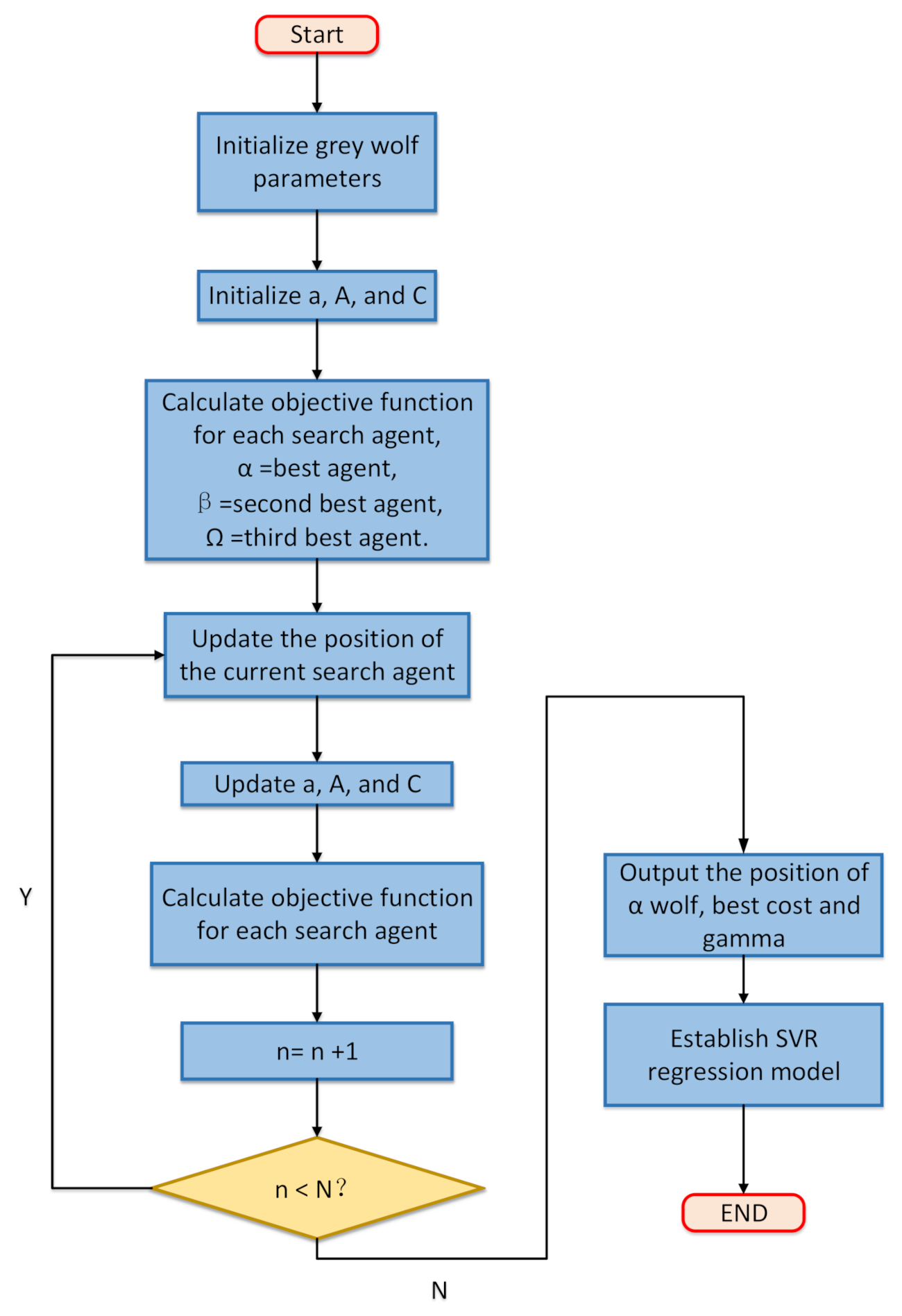The Figure 1 is the algorithm flow chart of GWO-SVR. The steps for GWO to optimize SVR parameters are as follows:

Step 1: Set the parameters of the GWO optimization algorithm, including initial population size M, the maximum number of iterations N, and the search range of cost parameters and gamma parameters.

Step 2: Initialize the position of each wolf in the wolf group; the position of the grey wolf is determined by the values of the cost parameter and gamma parameter. Set synergy parameters a, A, and C, where |A| > 1 forces wolf and prey separation, 0 < |C| <2, and a are linearly decreased from 2 to 0 over the course of iterations.

Step 3: Calculate the fitness of the corresponding parameters of each wolf. According to the numerical order of fitness, the grey wolf is divided into four classes: α, β, δ, and ω.

Step 4: According to Equations (12)–(17), update the position of each grey wolf in the wolf group. Compare the fitness of the corresponding parameters in the new position of the grey wolf with that before the update to determine whether to replace the fitness. $\overrightarrow{D}$ represents the distance between grey wolf and prey, ${\overrightarrow{X}}_{\alpha }$, ${\overrightarrow{X}}_{\beta }$, and ${\overrightarrow{X}}_{{}_{\delta }}$ represent the position of the grey wolf of different classes, $\overrightarrow{X}$ represents the position of prey.

$${\overrightarrow{D}}_{\alpha }=|{\overrightarrow{C}}_1.{\overrightarrow{X}}_{\alpha }-\overrightarrow{X}|$$

(12)

$${\overrightarrow{D}}_{\beta }=|{\overrightarrow{C}}_2.{\overrightarrow{X}}_{{}_{\beta }}-\overrightarrow{X}|$$

(13)

$${\overrightarrow{D}}_{\delta }=|{\overrightarrow{C}}_3.{\overrightarrow{X}}_{{}_{\delta }}-\overrightarrow{X}|$$

(14)

$${\overrightarrow{X}}_1={\overrightarrow{X}}_{\alpha }-{\overrightarrow{A}}_1.(\overrightarrow{D_{\alpha }})$$

(15)

$${\overrightarrow{X}}_2={\overrightarrow{X}}_{\beta }-{\overrightarrow{A}}_2.(\overrightarrow{D_{\beta }})$$

(16)

$${\overrightarrow{X}}_3={\overrightarrow{X}}_{\delta }-{\overrightarrow{A}}_3.(\overrightarrow{D_{\delta }})$$

(17)

$$\overrightarrow{X}(t+1)=\frac{{\overrightarrow{X}}_1+{\overrightarrow{X}}_2+{\overrightarrow{X}}_3}{3}$$

(18)

Step 5: Update a, A, and C values.

Step 6: Calculate the fitness of the current parameters for each wolf.

Step 7: Determine whether the current iteration number is n < N; if not, output the global optimal value. If so, return to Step 4.

Step 8: Output the position of α wolf. The corresponding position of α wolf is the optimal cost parameter and gamma parameter.

Step 9: Establish the SVR regression model using the optimal cost parameters and gamma parameters.

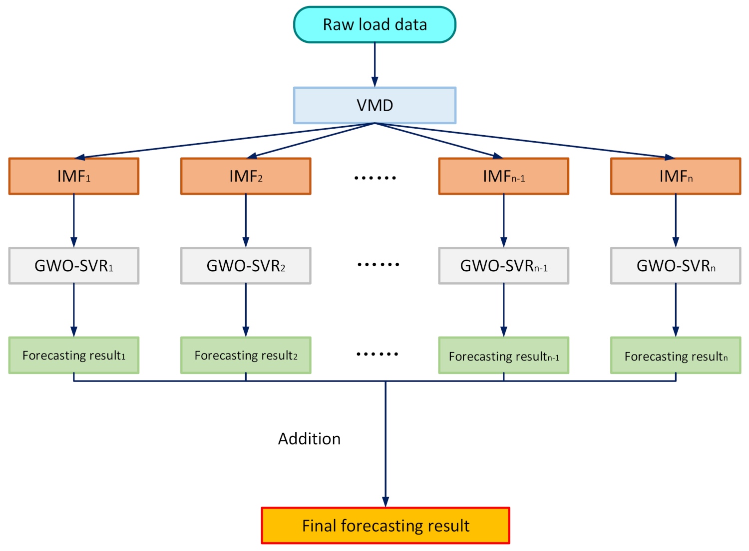
3.3. VMD-GWO-SVR

Figure 2 is the framework of the proposed method. First, the load series is decomposed into several high-frequency components and low-frequency components by VMD, and then each component is input into the GWO-SVR model for prediction. Finally, the predicted value of each component is superimposed to obtain the final prediction result.

3.4. Model Evaluation Indicators

In this study, the evaluation index is used to evaluate the performance of the prediction model. These indicators are mean absolute error (MAE), mean absolute percentage error (MAPE), mean square error (MSE), and determination coefficient (R²).

$$\mathrm{MAE}=\frac{{{\displaystyle {\sum }_{t=1}^M(L_t-{\widehat{L}}_t)}}^2}{M}$$

(19)

$$\mathrm{MAPE}=\frac{{\displaystyle {\sum }_{t=1}^M\frac{|(L_t-{\widehat{L}}_t)|}{L_t}}}{M}\times 100\%$$

(20)

$$\mathrm{MSE}=\frac{{\displaystyle {\sum }_{i=1}^M{\left(L_t-{\widehat{L}}_t\right)}^2}}{M}$$

(21)

$${\mathrm{R}}^2=1-\frac{{{\displaystyle {\sum }_{t=1}^M\left(L_t-{\widehat{L}}_t\right)}}^2}{{{\displaystyle {\sum }_{t=1}^M\left(L_t-{\overline{L}}_t\right)}}^2}$$

(22)

$$\mathrm{Adjusted} {\mathrm{R}}^2=1-\frac{\left(1-{\mathrm{R}}^2\right)\left(M-1\right)}{M-p-1}$$

(23)

where $L_t$ and ${\widehat{L}}_t$ are the actual and forecasting values of the load at time $t$, $M$ is the total number of data used, and $p$ is the number of features.

4. Data Sets

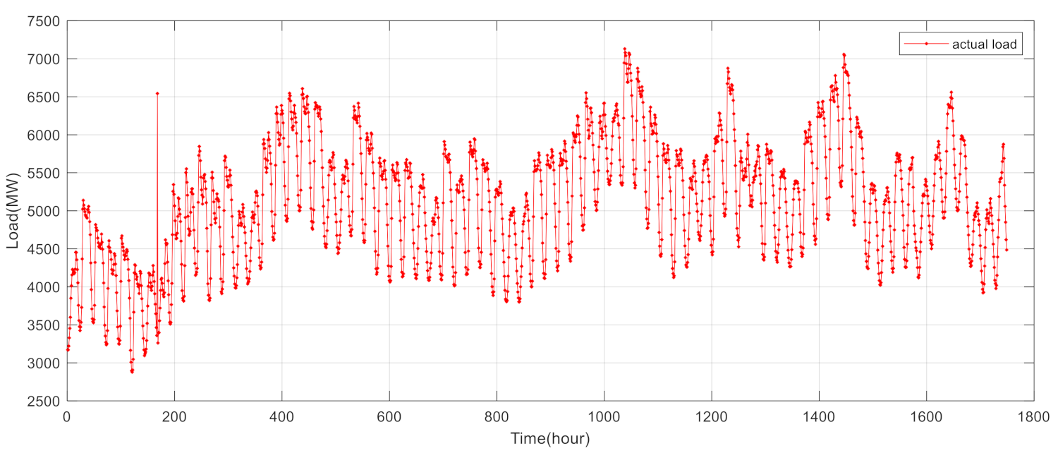
To verify the accuracy of the proposed model, we use the hourly load data of the grid in Oslo and its surrounding areas in 2019 [50] as the experimental data. It is found that 96 groups of load values are missing in February, and one group of load values is missing in March. Therefore, this paper uses the expectation-maximization method to fill the missing data. Through analysis of the filled data, it can be seen that the electricity consumption in January, February, and December is larger, and the electricity consumption in June, July, and August is smaller, as shown in

Table 2. Statistical information table of load data after filling.

Month	Max	Median	Min	Mean	Var	Std
January	7624	5998	4126	5918.09	604,428.6	777.45
February	7250	5351.5	3980	5414.76	593,896.8	770.65
March	6717	4834	1636	4878.71	485,349.9	696.67
April	5569	3729	2295	3723.60	498,868.4	706.31
May	4944	3289.5	1985	3263.81	330,654.9	575.03
June	3808	2839	1880	2879.67	190,646.5	436.63
July	3311	2501	1701	2487.02	135,150.4	367.63
August	3606	2900.5	1693	2815.10	232,623	482.31
September	4396	3460.5	2055	3379.94	237,244.4	487.08
October	6543	4152	2879	4146.16	373,954.7	611.52
November	6607	5266	3803	5204.88	481,819.8	694.13
December	7131	5386.5	3921	5393.85	513,362.7	716.49

.

In this paper, the experimental data is divided into the training set and the prediction set according to the ratio of 4:1. The first 7008 h of data are used as the training set, and the rest of the data are used as the prediction set. We divide the load data into groups every four hours and forecast the load value of the next hour through the load data of the first three hours. Therefore, the number of features in this paper is three.

Combined with Figure 3, we can see that the load value shows a downward trend from January to August, reaching the lowest electricity consumption in August, and the load value shows an upward trend from August to December. Through the variance and standard deviation, we find that the January, February, April, and December load value fluctuations are larger, whereas the June, July, August, and September load fluctuations are smaller.

Experiments were conducted on 64-bit Windows 10 using MATLAB R2018a with an i7-7700hq CPU and a GTX-1050 graphics card.

5. Results and Discussion

5.1. Variational Mode Decomposition

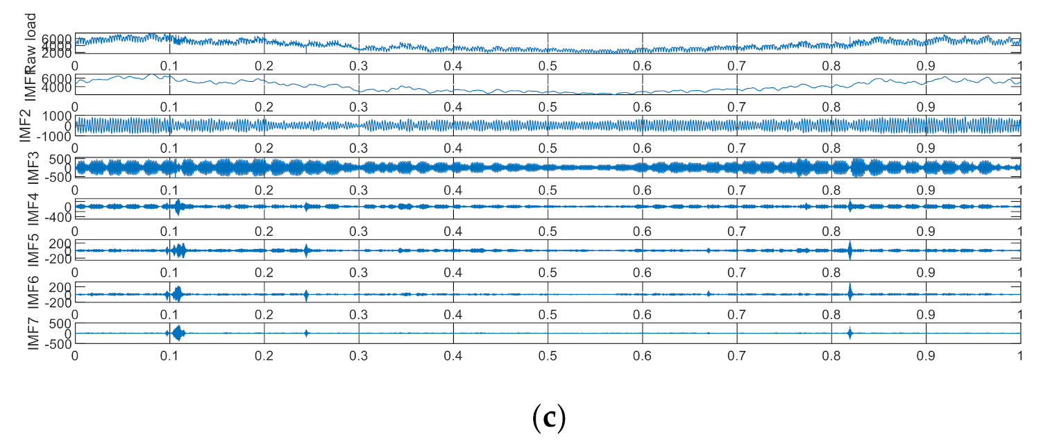
The VMD algorithm needs to set the number of decomposition modes K in advance. In this paper, the K value is determined by observing the central frequency of each mode. If the central frequency is similar to the modal component, it is considered that VMD has over-decomposition. Figure 4 shows the decomposition results of three cases with K values of 5, 6, and 7.

Table 3. IMF central frequencies at K = 2, 3, 4, 5, 6, and 7.

K	IMF1	IMF2	IMF3	IMF4	IMF5	IMF6	IMF7
2	2.17 × 10−5.	0.0917
3	2.14 × 10−5.	0.0806	0.2325
4	2.14 × 10−5.	0.0775	0.2022	0.3915
5	1.92 × 10−5.	0.0797	0.1158	0.2256	0.4209
6	1.76 × 10−5.	0.0816	0.0624	0.2070	0.3274	0.4242
7	1.67 × 10−5.	0.0432	0.0868	0.2042	0.2602	0.3380	0.4258

shows the modal center frequencies of different modal decompositions. The results of modal decomposition show that when the number of decomposed modes is 6, the waveforms of IMF5 and IMF6 are similar and the center frequencies are 0.327434 and 0.424177, respectively. When K = 7, the waveforms of IMF4, IMF5, IMF6, and IMF7 are similar, and the central frequencies are 0.2042, 0.2602, 0.3380, and 0.4258, respectively. Therefore, it can be determined that over-decomposition occurs when K > 5, so K = 5.

It can be seen from Figure 4 that the power consumption of IMF1 after decomposition is the smallest in June, July, and August and the largest in January, February, and December, which is in line with the law before the decomposition of load data. On the other hand, the load data can be regarded as composed of several high-frequency components and low-frequency components. The load has relatively complex data characteristics, and the load characteristics at different scales can be better displayed by modal decomposition.

5.2. Influence of Each Modal Component on Electric Load Forecasting Results

In order to further explore the influence of the prediction results for each component, we summarize the prediction effect of GWO and artificial bee colony algorithm optimized SVR models for five components after VMD decomposition, as shown in

Table 4. Prediction results of the ABC-SVR model and GWO-SVR model for five components.

	GWO-SVR					ABC-SVR
	MAE (MW)	MAPE (%)	MSE	R2	Adjusted R2	MAE (MW)	MAPE (%)	MSE	R2	Adjusted R2
IMF1	24.71	0.47	918.40	0.9970	0.9970	24.71	0.47	918.40	0.9970	0.9970
IMF2	10.32	41.91	188.90	0.9958	0.9958	10.33	41.91	188.92	0.9958	0.9958
IMF3	25.97	38.17	1067.90	0.9949	0.9949	26.03	36.94	1067.85	0.9949	0.9949
IMF4	4.94	64.41	49.28	0.9764	0.9764	5.01	72.57	48.53	0.9767	0.9767
IMF5	1.39	81.94	9.16	0.9782	0.9782	1.40	81.94	9.16	0.9781	0.9781

. We can see that the prediction effect of GWO on IMF1 and IMF2 is almost the same as that of ABC. Among the five indicators predicted by IMF3, MSE and MAPE of ABC are better than those of GWO; R² and Adjusted R² are the same as that of GWO; and MAE is slightly worse than that of GWO. In the prediction of IMF4 by GWO, MAE, and MAPE were better than ABC; MSE, R², and Adjusted R² were slightly worse than ABC. For the prediction results of IMF5, the MSE and MAPE of GWO-SVR and ABC-SVR are the same, but the MAE, R², and Adjusted R² of GWO-SVR are better than ABC-SVR. Thus, we can conclude that GWO-SVR and ABC-SVR have similar prediction performance in low-frequency components, but GWO-SVR has higher prediction accuracy in high-frequency components. Through five indexes we can see that the difficulty of the prediction increases with the increase of component frequency.

To better compare the performance of the two models, we also compare the training time and predicting time of the two models. As shown in

Table 5. Model calculation time and parameter selection.

	GWO-SVR				ABC-SVR
	Training Time (s)	Predicting Time (s)	Cost	Gamma	Training Time (s)	Predicting Time (s)	Cost	Gamma
IMF1	9.71	0.043	64.37	0.05	89.54	0.049	70.56	0.05
IMF2	50.37	0.042	38.60	0.20	159.31	0.037	42.53	0.20
IMF3	46.67	0.005	66.20	6.32	140.46	0.005	82.97	6.40
IMF4	205.12	0.003	35.59	0.06	395.38	0.040	11.36	0.51
IMF5	97.05	0.003	91.23	0.78	143.00	0.004	72.50	0.78

, the training time and predicting time of the GWO-SVR model for each component are shorter than those of ABC-SVR. For IMF1, IMF2, and IMF3, the prediction accuracy of ABC-SVR and GWO-SVR are the same, but the training times of the GWO-SVR model are shorter than that of the ABC-SVR model. At this time, the values of the GWO-SVR model cost parameter and the values of the gamma parameters of the GWO-SVR model are 64.37, 0.05; 38.60, 0.20; 66.20, 6.32. For IMF4 and IMF5, the prediction accuracy of the GWO-SVR model is higher than that of the ABC-SVR, and the model training time is shorter than that of the ABC-SVR; the values of the cost and gamma parameters of the GWO-SVR model are 35.59, 0.06; 91.23, 0.78. Considering the prediction accuracy and computation time together, we can conclude that the prediction performance of VMD-GWO-SVR is better than that of VMD-ABC-SVR.

As shown in

Table 6. Statistical characteristics of each component.

	MAX	MEDIAN	MIN	MEAN
IMF1	6347.684	5121.461	3770.904	5138.844
IMF2	561.3764	−2.66641	−538.527	−0.04058
IMF3	842.0584	−2.02205	−781.989	−0.2385
IMF4	350.044	0.603477	−266.968	0.002172
IMF5	365.1115	−0.02622	−311.027	−0.00084

, we can see that the low-frequency component often has a larger value, which has a greater impact on the accuracy of electric load forecasting results.

5.3. Comparison of GWO-SVR Combined with Different Modal Decomposition Methods

In order to compare the influence of different modal decomposition methods and to determine whether to use the modal decomposition method for electric load forecasting, the data processed by EMD and the data without modal decomposition are compared with the data processed by variational mode decomposition. The regression algorithm adopts the GWO-SVR algorithm. The initial population number for GWO optimization is set to 30, and the optimization range of the cost parameter and gamma parameter is set to [0.01, 100]. The

Table 7. Prediction results of different modal decomposition methods combined under the GWO-SVR model.

Algorithm	Training Time (s)	Predicting Time (s)	MAE (MW)	MAPE (%)	MSE	R2
GWO-SVR	2703.05	0.072	101.16	1.96	22,534.11	0.9643
EMD-GWO-SVR	2609.72	0.123	72.62	1.47	14,146.04	0.9776
VMD-GWO-SVR	408.92	0.096	71.65	1.41	10,461.32	0.9834

shows the GWO-SVR prediction results under different modal decompositions. The training time in the table is the sum of the training time of the model for the five components, and the predicting time is the sum of the predicting times for the five components.

Through the analysis, we can see that the prediction results for the MAE, MAPE, and MSE of GWO-SVR with mode decomposition are reduced compared with those without mode decomposition, and the determination coefficient R² is increased from 0.9643 to 0.9776 and 0.9834, which shows that the load series decomposition with mode decomposition is helpful to improve the accuracy of electric load forecasting. Through the comparison between VMD decomposition and EMD decomposition, it can be found that MAE decreases by 0.9729, MAPE decreases by 0.57%, MSE decreases by 3684.72, and R² increases by 0.0058. It can be seen that VMD has a better effect than EMD in the field of electric load forecasting.

On the other hand, we can see that the training time of the VMD-GWO-SVR model is significantly shorter than the other two algorithms by comparing the predicting time and testing time of the three models. The predicting time is 0.024 s longer than that of GWO-SVR. Considering the prediction accuracy and computation time, we can determine that the prediction performance of VMD-GWO-SVR is better than that of EMD-GWO-SVR and GWO-SVR.

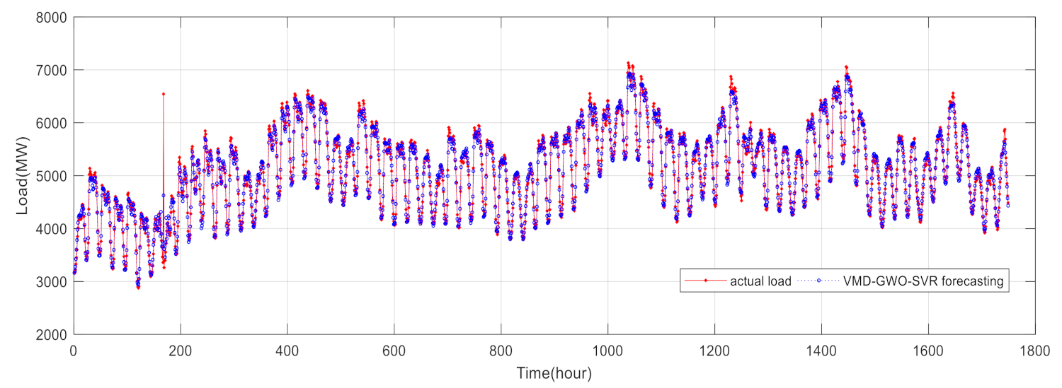
It can be seen from Figure 5 that VMD-GWO-SVR has a good prediction effect. The trend of the predicted value and the actual value of this model is the same (R² is 0.9834), and the prediction error is small (MAE is 71.6453, MAPE is 0.1413, and MSE is 10461.32). Therefore, this model has high prediction accuracy.

5.4. Comparison of Variational Modal Decomposition Combined with Different Optimization Algorithms

In order to verify the accuracy of the proposed method in the field of short-term electric load forecasting, this paper not only makes a longitudinal comparison with the prediction results of the SVR without the optimization algorithm but also compares it with the prediction results of the SVR algorithm using the GA, PSO and ABC. The initial population of the genetic optimization algorithm, particle swarm optimization algorithm, and artificial bee colony optimization algorithm is set to 30, the maximum number of iterations is set to 100, the search range of cost parameters and gamma parameters is set to [0.01, 100], and the load value is normalized to [−1, 1]. The above work ensures the unity of initial conditions. It can be seen that the GWO-SVR and SVR prediction results have been improved under the premise of using VMD for modal decomposition, which proves that the use of the modal decomposition method is helpful to improve the accuracy of electric load forecasting. By comparing the prediction results of GWO use for optimization of SVR parameters, we find that the prediction accuracy of the SVR model optimized by GWO under the premise of modal decomposition is significantly improved, and MAE is reduced by 62.5705 compared with VMD-SVR, which is only 53.4% of VMD-SVR. MAPE decreases by 0.01242 compared with VMD-SVR, which is only 53.2% of VMD-SVR. MSE decreases by 17,347.3592 compared with VMD-SVR, which is only 37.7% of VMD-SVR. R² increases by 0.027. Based on the above analysis, we can draw the conclusion that parameter optimization of the SVR model using an optimization algorithm is helpful to improve the prediction accuracy.

The training time in specified in

Table 8. SVR model combined with GWO optimization prediction results.

Algorithm	Training Time (s)	Predicting Time (s)	MAE (MW)	MAPE (%)	MSE	R2
SVR	0.26	0.011	134.72	2.72	42,147.76	0.9333
VMD-SVR	0.08	0.018	134.22	2.66	27,808.68	0.9560
GWO-SVR	2703.05	0.072	101.16	1.96	22,534.11	0.9643
VMD-GWO-SVR	408.92	0.096	71.65	1.41	10,461.32	0.9834

is the sum of the training times of the models for the five components, and the predicting time is the sum of the predicting times for the five components. By comparing the predicting time and training time of SVR and VMD-SVR and comparing the predicting time and training time of GWO-SVR and VMD-GWO-SVR, we can see that using VMD to decompose the original load series not only improves the prediction accuracy of the model but also reduces the computation time of the model. Among the four models mentioned above, VMD-GWO-SVR has the highest prediction accuracy, and the model training time is longer than that of VMD-SVR, but the three indexes of MAE, MAPE, and MSE have more obvious advantages than VMD-SVR. Considering the prediction time and accuracy, VMD-GWO-SVR is more suitable for short-term electric load forecasting.

Table 9. VMD combined with different optimized SVR model prediction results.

Algorithm	MAE (MW)	MAPE (%)	MSE	R2
GA-SVR	202.51	3.90	60,543.58	0.9041
PSO-SVR	114.28	2.24	23,825.86	0.9623
ABC-SVR	85.73	1.66	14,699.52	0.9767
GWO-SVR	71.65	1.41	10,461.32	0.9834

shows the prediction results of different optimization algorithms combined with SVR after VMD modal decomposition. It can be seen that the prediction accuracies of ABC-SVR and GWO-SVR are relatively close. The prediction accuracy of PSO-SVR is lower than that of ABC-SVR and GWO-SVR, and the prediction accuracy of GA-SVR is the worst. Further comparison of the four evaluation indexes of ABC-SVR and GWO-SVR shows that MAE, MAPE, and MSE of GWO-SVR are smaller, indicating that the predicted results are closer to the actual load value than ABC-SVR. The R² of 0.9834 is greater than 0.9767 of ABC-SVR, indicating that the trend of GWO-SVR prediction results is closer to the trend of actual load value than that of ABC-SVR. In summary, we can conclude that GWO-SVR has higher accuracy in the field of electric load forecasting than SVR optimized by other optimization algorithms, and it can also better predict the trend of actual load value change.

6. Conclusions

In this paper, a prediction model based on the “decomposition and integration” method combined with VMD and GWO-SVR is proposed. First, the load series is decomposed by VMD, and the optimal modal number K = 5 is selected by observing the central frequency of the component combined with the component waveform. Then, the five decomposed components are input into the GWO-SVR model for parameter optimization. Finally, the five prediction results are superimposed to obtain the final prediction results. In this paper, the proposed method is compared with other prediction methods. The 2019 hourly load data of the first landmark area of Norway, Oslo, and its surrounding areas are used. The conclusions are as follows:

(1) Modal decomposition of the load series can effectively separate the complex information contained in the original series and then predict each component separately, which helps to improve the prediction accuracy of the model and the prediction ability of the load value trend. Regarding the load data decomposition method, VMD decomposition can better separate the feature information from the original series into different components. In addition, the decomposition of the load series using VMD can also effectively reduce the model computation time.

(2) Compared with other optimization algorithms after VMD processing, the GWO-SVR algorithm is the best in all four indicators. Compared with ABC’s five component prediction results, GWO’s prediction results in IMF1–IMF3 are almost the same, but it has better prediction effect on IMF4 and IMF5, indicating that GWO has better accuracy in high-frequency component prediction. On the other hand, the computation time of VMD-GWO-SVR for all five components is shorter than that of the corresponding components of VMD-ABC-SVR.

(3) This method has high accuracy in electric load forecasting and can better predict the trend of load change, which indicates that this method has good application prospect for short-term electric load forecasting.

In future work, we will investigate the delay between time series and apply other methods to deal with the high-frequency components of the modal decomposition in order to further improve the accuracy of the model.

References

- Nezamabad, H.A.; Zand, M.; Alizadeh, A.; Vosoogh, M.; Nojavan, S. Multi-objective optimization based robust scheduling of electric vehicles aggregator. Sustain. Cities Soc. 2019, 47, 101494. [Google Scholar] [CrossRef]
- Aguayo-Alquicira, J.; Vásquez-Libreros, I.; De Léon-Aldaco, S.; Ponce-Silva, M.; Lozoya-Ponce, R.; Flores-Rodríguez, E.; García-Morales, J.; Reyes-Severiano, Y.; Carrillo-Santos, L.; Marín-Reyes, M.; et al. Reconfiguration Strategy for Fault Tolerance in a Cascaded Multilevel Inverter Using a Z-Source Converter. Electronics 2021, 10, 574. [Google Scholar] [CrossRef]
- Rohani, A.; Joorabian, M.; Abasi, M.; Zand, M. Three-phase amplitude adaptive notch filter control design of DSTATCOM under unbalanced/distorted utility voltage conditions. J. Intell. Fuzzy Syst. 2019, 37, 847–865. [Google Scholar] [CrossRef]
- Zand, M.; Nasab, M.A.; Hatami, A.; Kargar, M.; Chamorro, H.R. Using Adaptive Fuzzy Logic for Intelligent Energy Management in Hybrid Vehicles. In Proceedings of the 2020 28th Iranian Conference on Electrical Engineering (ICEE), Tabriz, Iran, 4–6 August 2020; pp. 1–7. [Google Scholar]
- Zikria, Y.; Ali, R.; Afzal, M.; Kim, S. Next-Generation Internet of Things (IoT): Opportunities, Challenges, and Solutions. Sensors 2021, 21, 1174. [Google Scholar] [CrossRef]
- Zand, M.; Nasab, M.A.; Neghabi, O.; Khalili, M.; Goli, A. Fault locating transmission lines with thyristor-controlled series capacitors By fuzzy logic method. In Proceedings of the 2020 14th International Conference on Protection and Automation of Power Systems (IPAPS), Tehran, Iran, 31 December 2019–1 January 2020; pp. 62–70. [Google Scholar]
- Upadhaya, D.; Thakur, R.; Singh, N.K. A systematic review on the methods of short term load forecasting. In Proceedings of the 2019 2nd International Conference on Power Energy, Environment and Intelligent Control (PEEIC), Greater Noida, India, 18–19 October 2019; pp. 6–11. [Google Scholar]
- Kuster, C.; Rezgui, Y.; Mourshed, M. Electrical load forecasting models: A critical systematic review. Sustain. Cities Soc. 2017, 35, 257–270. [Google Scholar] [CrossRef]
- Dragomiretskiy, K.; Zosso, D. Variational Mode Decomposition. IEEE Trans. Signal. Process. 2014, 62, 531–544. [Google Scholar] [CrossRef]
- Aneesh, C.; Kumar, S.; Hisham, P.; Soman, K. Performance Comparison of Variational Mode Decomposition over Empirical Wavelet Transform for the Classification of Power Quality Disturbances Using Support Vector Machine. Procedia Comput. Sci. 2015, 46, 372–380. [Google Scholar] [CrossRef] [Green Version]
- Sun, G.; Chen, T.; Wei, Z.; Sun, Y.; Zang, H.; Chen, S. A Carbon Price Forecasting Model Based on Variational Mode Decomposition and Spiking Neural Networks. Energies 2016, 9, 54. [Google Scholar] [CrossRef] [Green Version]
- Ferrari, V. Libsvm: A Library for Support Vector Machines. 2008. Available online: https://www.semanticscholar.org/paper/LIBSVM%3A-A-library-for-support-vector-machines-Chang-Lin/273dfbcb68080251f5e9ff38b4413d7bd84b10a1?p2df (accessed on 19 October 2019).
- Mirjalili, S.; Mirjalili, S.M.; Lewis, A. Grey Wolf Optimizer. Adv. Eng. Softw. 2014, 69, 46–61. [Google Scholar] [CrossRef] [Green Version]
- Cho, M.; Hwang, J.; Chen, C. Customer short term load forecasting by using ARIMA transfer function model. In Proceedings of the 1995 International Conference on Energy Management and Power Delivery EMPD ’95, Singapore, 21–23 November 1995; Volume 1, pp. 317–322. [Google Scholar]
- Lee, C.-M.; Ko, C.-N. Short-term load forecasting using lifting scheme and ARIMA models. Expert Syst. Appl. 2011, 38, 5902–5911. [Google Scholar] [CrossRef]
- Patel, H.; Pandya, M.; Aware, M. Short term load forecasting of Indian system using linear regression and artificial neural network. In Proceedings of the 2015 5th Nirma University International Conference on Engineering (NUiCONE), Ahmedabad, India, 26–28 November 2015; pp. 1–5. [Google Scholar]
- Song, K.-B.; Baek, Y.-S.; Hong, D.H.; Jang, G. Short-Term Load Forecasting for the Holidays Using Fuzzy Linear Regression Method. IEEE Trans. Power Syst. 2005, 20, 96–101. [Google Scholar] [CrossRef]
- Hong, T.; Wang, P.; Willis, H.L. A Naïve multiple linear regression benchmark for short term load forecasting. In Proceedings of the 2011 IEEE Power and Energy Society General Meeting, Detroit, MI, USA, 24–28 July 2011; pp. 1–6. [Google Scholar] [CrossRef]
- Amral, N.; Ozveren, C.S.; King, D. Short term load forecasting using Multiple Linear Regression. In Proceedings of the 2007 42nd International Universities Power Engineering Conference, Brighton, UK, 4–6 September 2007; pp. 1192–1198. [Google Scholar]
- Göb, R.; Lurz, K.; Pievatolo, A. Electrical load forecasting by exponential smoothing with covariates. Appl. Stoch. Model. Bus. Ind. 2013, 29, 629–645. [Google Scholar] [CrossRef]
- Rendon-Sanchez, J.F.; de Menezes, L.M. Structural combination of seasonal exponential smoothing forecasts applied to load forecasting—ScienceDirect. Eur. J. Oper. Res. 2019, 275, 916–924. [Google Scholar] [CrossRef]
- Manohar, T.G.; Reddy, V. Load forecasting by a novel technique using ANN. J. Eng. Appl. Sci. 2008, 3, 19–25. [Google Scholar]
- Jigoria-Oprea, D.; Lustrea, B.; Borlea, I.; Kilyeni, S.; Andea, P.; Barbulescu, C. Short term daily load forecasting using recursive ANN. In Proceedings of the EUROCON 2009, St. Petersburg, Russia, 18–23 May 2009. [Google Scholar]
- Hong, W.-C. Electric load forecasting by seasonal recurrent SVR (support vector regression) with chaotic artificial bee colony algorithm. Energy 2011, 36, 5568–5578. [Google Scholar] [CrossRef]
- Aly, H.H. A proposed intelligent short-term load forecasting hybrid models of ANN, WNN and KF based on clustering techniques for smart grid. Electr. Power Syst. Res. 2020, 182, 106191. [Google Scholar] [CrossRef]
- Chen, H.; Wang, S.; Wang, S.; Li, Y. Day-ahead aggregated load forecasting based on two-terminal sparse coding and deep neural network fusion. Electr. Power Syst. Res. 2019, 177, 105987.1–105987.12. [Google Scholar] [CrossRef]
- Mei, F.; Wu, Q.; Shi, T.; Lu, J.; Pan, Y.; Zheng, J. An Ultrashort-Term Net Load Forecasting Model Based on Phase Space Reconstruction and Deep Neural Network. Appl. Sci. 2019, 9, 1487. [Google Scholar] [CrossRef] [Green Version]
- Kong, W.; Dong, Z.Y.; Jia, Y.; Hill, D.J.; Xu, Y.; Zhang, Y. Short-Term Residential Load Forecasting Based on LSTM Recurrent Neural Network. IEEE Trans. Smart Grid 2019, 10, 841–851. [Google Scholar] [CrossRef]
- Wang, Y.; Gan, D.; Sun, M.; Zhang, N.; Lu, Z.; Kang, C. Probabilistic individual load forecasting using pinball loss guided LSTM. Appl. Energy 2019, 235, 10–20. [Google Scholar] [CrossRef] [Green Version]
- He, H.; Pan, J.; Lu, N.; Chen, B.; Jiao, R. Short-term load probabilistic forecasting based on quantile regression convolutional neural network and Epanechnikov kernel density estimation—ScienceDirect. Energy Rep. 2020, 6, 1550–1556. [Google Scholar] [CrossRef]
- Sadaei, H.J.; Silva, P.C.D.L.E.; Guimarães, F.G.; Lee, M.H. Short-term load forecasting by using a combined method of convolutional neural networks and fuzzy time series. Energy 2019, 175, 365–377. [Google Scholar] [CrossRef]
- Guo, X.; Zhao, Q.; Zheng, D.; Ning, Y.; Gao, Y. A short-term load forecasting model of multi-scale CNN-LSTM hybrid neural network considering the loda-time electricity price. Energy Rep. 2020, 6, 1046–1053. [Google Scholar] [CrossRef]
- da Silva, R.G.; Ribeiro, M.H.D.M.; Moreno, S.R.; Mariani, V.C.; Coelho, L.D.S. A novel decomposition-ensemble learning framework for multi-step ahead wind energy forecasting. Energy 2021, 216, 119174. [Google Scholar] [CrossRef]
- Liu, H.; Yang, R.; Wang, T.; Zhang, L. A hybrid neural network model for short-term wind speed forecasting based on decomposition, multi-learner ensemble, and adaptive multiple error corrections. Renew. Energy 2021, 165, 573–594. [Google Scholar] [CrossRef]
- Chaabi, L.; Lemzadmi, A.; Djebala, A.; Bouhalais, M.L.; Ouelaa, N. Fault diagnosis of rolling bearings in non-stationary running conditions using improved CEEMDAN and multivariate denoising based on wavelet and principal component analyses. Int. J. Adv. Manuf. Technol. 2020, 107, 3859–3873. [Google Scholar] [CrossRef]
- Xue, X.; Zhou, J.; Xu, Y.; Zhu, W.; Li, C. An adaptively fast ensemble empirical mode decomposition method and its applications to rolling element bearing fault diagnosis. Mech. Syst. Signal. Process. 2015, 62–63, 444–459. [Google Scholar] [CrossRef]
- Zhou, M.; Bian, K.; Hu, F.; Lai, W. A New Method Based on CEEMD Combined With Iterative Feature Reduction for Aided Diagnosis of Epileptic EEG. Front. Bioeng. Biotechnol. 2020, 8, 669. [Google Scholar] [CrossRef]
- Martis, R.J.; Acharya, U.R.; Min, L.C. ECG beat classification using PCA, LDA, ICA and Discrete Wavelet Transform. Biomed. Signal. Process. Control. 2013, 8, 437–448. [Google Scholar] [CrossRef]
- Li, S.; Wang, P.; Goel, L. Short-term load forecasting by wavelet transform and evolutionary extreme learning machine. Electr. Power Syst. Res. 2015, 122, 96–103. [Google Scholar] [CrossRef]
- Li, S.; Goel, L.; Wang, P. An ensemble approach for short-term load forecasting by extreme learning machine. Appl. Energy 2016, 170, 22–29. [Google Scholar] [CrossRef]
- Ding, J.; Wang, M.; Ping, Z.; Fu, D.; Vassiliadis, V.S. An integrated method based on relevance vector machine for short-term load forecasting. Eur. J. Oper. Res. 2020, 287, 497–510. [Google Scholar] [CrossRef]
- Kassa, Y.; Zhang, J.; Zheng, D. EMD-PSO-ANFIS based hybrid approach for short-term load forecasting in microgrids. IET Gener. Transm. Distrib. 2019, 14, 470–475. [Google Scholar]
- Jiang, W.; Wang, Z. Calibration of visual model for space manipulator with a hybrid LM–GA algorithm. Mech. Syst. Signal. Process. 2016, 66–67, 399–409. [Google Scholar] [CrossRef]
- Luque-Gallego, M.; Miettinen, K.; Saborido, R.; Ruiz, A.B. An Interactive Evolutionary Multiobjective Optimization Method based on the WASF-GA Algorithm. 2014. Available online: https://www.riuma.uma.es/xmlui/bitstream/handle/10630/7874/Presentacion_IFORS2014_RIUMA.pdf?sequence=1 (accessed on 4 April 2021).
- Jiao, B.; Lian, Z.; Gu, X. A dynamic inertia weight particle swarm optimization algorithm. Chaos Solitons Fractals 2008, 37, 698–705. [Google Scholar] [CrossRef]
- Assareh, E.; Behrang, M.; Assari, M.; Ghanbarzadeh, A. Application of PSO (particle swarm optimization) and GA (genetic algorithm) techniques on demand estimation of oil in Iran. Energy 2010, 35, 5223–5229. [Google Scholar] [CrossRef]
- Karaboga, D.; Basturk, B. A powerful and efficient algorithm for numerical function optimization: Artificial bee colony (ABC) algorithm. J. Glob. Optim. 2007, 39, 459–471. [Google Scholar] [CrossRef]
- Kumar, S.K.P.; Sumithra, M.G.; Saranya, N. Artificial bee colony-based fuzzy c means (ABC-FCM) segmentation algorithm and dimensionality reduction for leaf disease detection in bioinformatics. J. Supercomput. 2019, 75, 8293–8311. [Google Scholar] [CrossRef]
- Mustaffa, Z.; Sulaiman, M.H.; Kahar, M.N.M. Training LSSVM with GWO for price forecasting. In Proceedings of the 2015 International Conference on Informatics, Electronics & Vision (ICIEV), Fukuoka, Japan, 15–18 June 2015; pp. 1–6. [Google Scholar]
- Zhang, S.; Wang, Y.; Zhang, Y.; Wang, D.; Zhang, N. Load probability density forecasting by transforming and combining quantile forecasts. Appl. Energy 2020, 277, 115600. [Google Scholar] [CrossRef]