Numerical Investigation of Major Impact Factors Influencing Fracture-Driven Interactions in Tight Oil Reservoirs: A Case Study of Mahu Sug, Xinjiang, China

Abstract

Fracture-driven interactions (FDIs) in unconventional reservoirs significantly affect well production and have thus garnered extensive attention from the scientific community. Furthermore, since the industry transitioned to using large completion designs with closer well spacing and infill drilling, FDIs have occurred more frequently and featured more prominently, which has primarily led to destructive interference. When infill wells (i.e., “child” wells) are fractured, older, adjacent producing wells (i.e., “parent” wells) are put directly at risk of premature changes in production behavior. Some wells may never fully recover following exposure to severe FDIs and, in the worst case scenario, will permanently stop producing. To date, previous investigations into FDIs have focused mainly on diagnosis and detection. As such, their formation mechanism is not well understood. To address this deficiency, a three-dimensional, multi-fracture propagation simulator was constructed based on the unconventional fracture model (UFM) and applied to a system that included both an older, adjacent passive well (“parent” well) and an active well (“child” well). Herein, the theoretical framework for overall complex fracture modeling is described. Furthermore, numerical simulation results are presented, demonstrating the critical roles of in-situ stress distribution and pre-existing natural fractures and aiding in the development of appropriate strategies for managing FDIs.

1. Introduction

Advances in drilling and fracturing technologies have facilitated new, unconventional reservoir design trends that consist of large-scale completions with more horizontal cluster wells and multi-stage fracturing. The more tightly spaced the wells become, the greater the risk of fracture-driven interactions (FDIs), because hydraulic fractures (HFs) between wells are easily communicated [1]. Recently, FDIs have increased in both prominence and frequency and have thus become a focal point of both the industrial and scientific communities [2]. FDIs associated with infill wells that are adjacent or near-adjacent to production wells are known for being problematic, as they initiate (1) abnormal changes in wellhead pressure, daily gas/oil production, and daily water production; and (2) water flooding, mud backflow, and/or sand production, etc. In the most severe circumstances, the affected production well may never fully recover and may even permanently stop producing.

Historically, this relationship has been characterized using a variety of terminology. For example, the concept of a “child” well (i.e., tightly spaced, newly completed offset well) interfering with a “parent” well (existing producer well) has been referred to as “inter-well interference”, “frac bashing”, “frac hit”, or “frac intersection”, among other terms. In 2013, Merkle et al. [3] proposed a conceptual model to describe the distribution and redistribution of injected fluid that includes the following three phases—pre-flowback “set up” phase, initial flowback “pinch off” phase, and long term “established production” phase. Subsequently, Sardinha et al. [4] distinguished the differences between the basic types of fracture hits by analyzing pre-flowback pressure interactions. In summary, they identified and presented three types of pressure hits, known as “fracture shadow”, “direct hit”, and “variable hit”, the last of which is believed to reflect a complex, highly stimulated network between wells. Tang et al. [5] divided fracture hits into two categories based on the location of their occurrence (near wellbore region, stimulated reservoir volume); Cao et. al. [6] further subdivided these categories and identified four periods and five locations with the potential to cause inter-well interference. To define the broader overall subject, Daneshy and King [2] introduced the term “fracture-driven interaction (FDI)” and divided FDIs into two categories consisting of “fracture shadowing” and “frac/frac connections.” In this study, “frac/frac connection” FDIs were further subdivided into the following two groups according to their interaction media: (1) those with conductive fracture pathways between wells, including faults, natural fractures (NFs), and hydraulic fracture networks; and (2) those that occur in the rock matrix.

With respect to the three phases comprising Merkle’s conceptual model, most of the interactions between wells are observed in the first two phases, thus providing useful data for identifying the type and intensity of the FDIs. In recent years, extensive empirical research studies have been conducted to aid the diagnosis and monitoring FDIs, and the results are expected to play a decisive role in the next generation of fracturing operations. To date, production data analysis (PDA), pressure interference testing, micro-seismic monitoring, fluid tracers, and proppant tracers have all been applied for this purpose. Among these testing technologies, PDA can directly quantify fracturing and production performance, while pressure interference tests offer information relating to connectivity between wells [7,8]. Although these two methods may be employed without constraints or cost, they are unable to provide direct and definitive evidence about the communication between wells. Therefore, a series of surveillance technologies, such as micro-seismic monitoring, fluid tracers, and proppant tracers, have been employed to provide information on fracture and proppant geometries, both of which reflect fracture conductivity and fracture connectivity between wells. Moreover, some new methods, such as controlled source electromagnetics (CSEM) and distributed optical fiber monitoring, have been applied to obtain a better understanding of the connections between wells [9,10]. These field observations substantiate some valuable conclusions and indicate that: (1) horizontal, multi-stage, multi-cluster fracturing results in the development of a highly complex fracture system when applied to formations that are characterized by fracture systems of different scales (NFs, faults, and planes of weakness) and pre-existing heterogeneity; (2) in most cases, FDIs in the rock matrix are insignificant, and frac/frac connections between active and passive wells are often destructive; (3) frac/frac connections through the fracture system pathways can remain conductive and cause damage to passive wells for a long time after the fracturing event; and (4) multiple fractures in a single perforation section often show a non-uniform propagation pattern, making it difficult to accurately control each fracture path during horizontal, multi-stage, multi-cluster fracturing.

FDIs between wells are often associated with complex fracture-propagation patterns. The state of in-situ stress changes when multiple fractures are synchronously generated, as this affects the extension path and fluid distribution of each fracture [11]. In some cases, a large amount of fluid is injected into the dominant fractures, which results in an excessive extension to adjacent wells. Furthermore, the pressure-depleted region around the production well lowers the stress level, which causes HFs in adjacent wells to expand into this region [12,13,14]. In general, HFs tend to intercept aged production wells or their vicinity, and the probability of this appearance primarily depends on the depth of the horizontal well, its location, and the extent of HFs [15]. The main challenge requires a deeper understanding of complex HF propagation with a consideration of heterogeneities occurring at various scales in the geological formations [16]. Heterogeneous distribution of in-situ stress has been identified as one of the most important factors associated with the increasing incidence of FDIs [17]. Moreover, due to the way in which HFs and NFs interact, the fracture networks between wells often develop into complex patterns that complicate the FDIs.

The investigation in this work was motivated by two aspects. Firstly, FDIs are basically well-to-well communications [18], and the frac/frac connections often lead to long-term effects. To avoid negative effects, it is important to develop a better understanding of complex-fracture growth and the geometry of fractures. Although numerous studies and simulations have been run in this field [19,20,21,22,23], research on patterns of complex-fracture growth between wells is still in its infancy. Therefore, a detailed analysis is needed to understand the inter-well HF geometry and, subsequently, to characterize FDIs. Secondly, influences on the different aspects of variables (treatment, completion, reservoir) pertaining to the hydraulic-fracture geometry have been emphasized in previous works [24,25]. However, the heterogeneous distribution of in-situ stress and natural fractures, both key factors affecting frac/frac connections, have not been treated with enough importance and their impacts remain unclear. Therefore, the impacts of these two variables require more in-depth investigation.

This study was designed to focus on FDIs that interact through conductive fracture pathways, and it specifically considers the interactions between HFs, adjacent HFs, and NFs. Herein, simulations were performed using the unconventional fracture model (UFM) to obtain a better understanding of the complex fracture networks that are formed between wells. The hydraulic fracture crossing model was also integrated, and the stress shadow effect was considered. Computational efficiency was maintained throughout the investigation. In addition, an expanded workflow—including fracture modeling, geomechanics modeling, and coupled flow (matrix and fracture)—was used in the numerical model to simulate the dynamic changes associated with in-situ stress variations resulting from pressure depletion in the production wells. Finally, the impacts of NF parameters on the fracture networks between wells were quantified and analyzed.

2. Field Observations and Questions

The Triassic Baikouquan formation’s Mahu 131 block is structurally located on the north slope of Mahu sag, the central depression of the Junggar basin. Lithology and electrical characteristics were previously used to divide the formation into three sections consisting, from bottom to top, of T₁b₁, T₁b₂, and T₁b₃. T₁b₂ is composed of two sand beds, known as T₁${\mathrm{b}}_2^1$ and T₁${\mathrm{b}}_2^2$, and the oil reservoir is mainly distributed in T₁b₃ and T₁${\mathrm{b}}_2^1$ (Figure 1a).

Reservoir lithologies primarily consist of gray sandy conglomerate, pebbly coarse sandstone, sandy conglomerate, and medium coarse and calcareous sandy conglomerate, etc. Statistical results of rock thin sections obtained from 10 wells indicate that these wells are composed of 57.1% gravel, 36.9% sandy component, 4.3% miscellaneous base, and 1.3% cement (Figure 1b). The T₁b₃ section exhibits an average porosity and permeability of 8.26% (5~14.3%) and 0.89 md (0.02~17.2 mD), respectively, while those of T₁${\mathrm{b}}_2^1$ are 7.63% (5~13.9%) and 1.33 mD (0.02~9.4 mD), respectively. According to the conglomerate reservoir classification scheme, these sections are considered ultra-low porosity and low-permeability reservoirs and, therefore, must be subjected to fracture stimulation for use in commercial production.

In October 2016, horizontal wells with long laterals were drilled into the Baikouquan formation and subjected to multi-stage fracturing with large amounts of slick water and sand. Severe inter-well interference complications developed as a response. To date, 92 horizontal oil wells have been put into production and 54.3% of them have interfered with adjacent wells. Of the total 1870 fracture-stimulated stages, 140 interfered in fracture treatments and 131 block accounts for 9.0%. As dictated by the hydraulic fracturing process for the adjacent active wells in the study area, the initial 16 stages of wells B, C, and D were fractured in the first fracture phase, while the remaining stages, including those of well A, were fractured in the second fracture phase. The inter-well, fracture-driven interactions that occurred in these areas share several common characteristics (Figure 2). First, the water production of passive wells (A, B, C and D) increased by a large magnitude when the adjacent active wells were stimulated. Second, the oil production rate sharply decreased in the fracture phase of the adjacent active wells. This behavior has been reported in Woodford, Eagle Ford, Bakken, and Horn River [4,26,27], but this is the first time it has been abundantly observed in Mahu. Finally, these production data showed evident, simultaneous variations in the passive wells in response to interference from active wells. Thus, it appears that passive wells are affected by the fracturing of adjacent active wells, which in turn indicates the existence of direct, high-conductivity pathways between them [11,28].

We used the method of production data analysis (PDA) to exclude the influence from adjacent active wells and try to illustrate this appearance [29]. An interpretation model of Passive Well A was built to estimate the change in fracture length following the two active well fracture phases (Figure 3). Rate-normalized pressure (RNA) analysis, which was based on the production data, provided average fracture half-length estimates of 85 and 103 m after the first and second FDI, respectively. The average well spacing is close to 200 m, making it likely that the conductive inter-well fracture network developed partially in response to the formation’s heterogeneity and NFs. Changes in the fracture half length were also observed in other passive wells after interference. In general, frac/frac connections between wells was the fundamental type of FDI observed in Mahu.

3. Methodology

Any investigation into FDIs between wells must overcome two primary challenges. First, the pressure-depleted region around the parent wells facilitates a heterogeneous distribution of in-situ stress. In turn, this phenomenon causes the child wells’ hydraulic fracture to propagate into the pressure-depleted region and creates direct, high-conductivity pathways across the wells. Second, the effects of existing NF networks and stress shadows should be considered when evaluating fracture propagation between multiple wells. The recently developed complex fracture model [30,31] offers a comprehensive solution to these challenges. Essentially, this model can be used to construct a series of numerical simulations that serve as the foundation for studying inter-well fracture interference. The design of this model was based on a complex fracture model and, as a result, the studies in which it is employed include a complete workflow or several of its components, such as geo-mechanical and reservoir properties, completion descriptions, fracture treatments, and production simulations [32,33]. In this case, to avoid the influence of other secondary factors, the key process was simplified; the geo-mechanical finite-element model (FEM) combined with the discrete fracture network (DFN) and complex hydraulic fracture models were used to simulate the spatial and temporal evolution of in-situ stress (Figure 4a). Furthermore, an expanded workflow proposed by Marongiu-Porcu (2015) was applied, which iterates the sequence of transversion for a depleted parent well and infill child well [33]. As illustrated in Figure 4b, the simulated in-situ stress field was imported as an initial condition of the child well, and the combined parent and child well reservoir simulation was developed afterwards.

3.1. UFM Description

The UFM used herein is a general complex fracture model that was recently developed by Weng et al. (2011) [30]. Built using similar principles to those of the commercial, cell-based, pseudo-3D (P3D) planar fracture model [34], this UFM effectively offers a fully coupled solution and is able to simulate the fracture propagation, rock deformation, and fluid flow in a complex fracture network. In contrast to the planar, full, three-dimensional fracture (PL3D) model, the hydraulic fracture in the cell-based P3D model is divided into a series of small, connected elements or cells with variable heights (Figure 5a). The fracture height is determined from the local net fluid pressure, vertical in-situ stress profile, and rock fracture toughness by satisfying the static equilibrium [35]. The application of this method circumvented the cumbersome computations required when using the PL3D model and thus significantly simplified the mathematics. Moreover, an extended crossing mode [36] was integrated in the UFM to calculate the interactions between the HFs and pre-existing NFs in complex fracture networks (Figure 5b). The following discussion provides a general description of the UFM and the process by which it was validated. UFM details can be found in Ching et al. (2015) [37].

3.1.1. Governing Equations

When simulating complex fracture-propagation patterns, various factors—such as fluid flow in the fracture network, fracture deformation, and fracture propagation—need to be considered [30]. As previously discussed, the complex fracture network in the UFM is divided into a series of small, connected elements or cells with variable heights that are constructed in a similar way to those in the P3D fracture model. Thus, the assumptions and governing equations in the UFM are the same as those in the P3D fracture model.

As illustrated in Figure 5a if it is assumed that the vertical in-situ stress distribution is piece-constant for a vertical fracture in the cell-based P3D fracture model, the fracture width at depth z in layer i can be determined using the elasticity equation [35]:

$$w\left(z\right)=\frac{4}{E^{\prime }}\left[p_{cp}-{\sigma }_n+{\rho }_{f}g\left(h_{cp}-\frac{h}{4}\right)\right]+\sqrt{\frac{2}{\pi h}}{\displaystyle \sum }_{i=1}^{n-1}\left({\sigma }_{i+1}-{\sigma }_i\right)\times \left[\frac{h}{2}arccos\left(\frac{h-2h_i}{h}\right)+\sqrt{z\left(h-z\right)}\right]$$

(1)

where $E^{\prime }$ is the Young’s modulus; ${\rho }_f$ is the fluid density; $p_{cp}$ is the pressure at perforation depth $h_{cp}$; ${\sigma }_n$ and ${\sigma }_i$ are the minimum horizontal principal stresses at the section and the layer $i$, respectively; and $h$ and $h_i$ are the fracture height and height of layer $i$, respectively, measured from the top to the lower tip.

In addition, fluid behavior in any element can be idealized as incompressible power-law fluid with index $n^{\prime }$ and consistency coefficient $K^{\prime }$, such that:

$$\frac{\partial p}{\partial s\left(x,y\right)}=-{\alpha }_0\frac{1}{{\overline{w}}^{2n^{\prime }+1}}\frac{q\left(t\right)}{h_{fl}}{\left|\frac{q\left(t\right)}{h_{fl}}\right|}^{n^{\prime }-1}$$

(2)

with

$${\alpha }_o=\frac{2K}{\phi {\left(n^{\prime }\right)}^{n^{\prime }}}{\left(\frac{4n^{\prime }+2}{n^{\prime }}\right)}^{n^{\prime }}; \phi \left(n^{\prime }\right)=\frac{1}{h_{fl}}\underset{h_{fl}}{\overset{}{{\displaystyle \int }}}{\left(\frac{w\left(z\right)}{\overline{w}}\right)}^{\frac{2n^{\prime }+1}{n^{\prime }}}dz$$

(3)

where $p$ and $q\left(t\right)$ are the fluid pressure and flow rate, respectively; $s\left(x,y\right)$ is the distance along the fracture; $\overline{w}$ is the average width; and $h_{fl}\left(s,t\right)$ is the current height of the fracture.

The local condition for mass balance was expressed using the continuity equation (Equation (4)) and validated by ensuring that the global volume balance satisfied Equation (5) [37]:

$$\frac{\partial p}{\partial s\left(x,y\right)}+\frac{\partial \left(h_{fl}\overline{w}\right)}{\partial t}+q_l\left(t\right)=0 ;q_l\left(t\right)=\frac{2h_l{c}_l}{\sqrt{t-{\tau }_0\left(s\right)}}, t>{\tau }_0\left(s\right)$$

(4)

$${{\displaystyle \int }}_0^{t}q\left(t\right)dt={{\displaystyle \int }}_0^{L\left(t\right)}h\left(s,t\right)\overline{w}ds+{{\displaystyle \int }}_{H_L}^{}{{\displaystyle \int }}_0^{L\left(t\right)}{{\displaystyle \int }}_0^t{q}_{l}dtdsd{h}_l$$

(5)

where $q_l\left(t\right)$ is the total leak-off rate of the fluid; $h_l$ is the height of the leak-off zone; $c_l$ is the total filtration coefficient; ${\tau }_0\left(s\right)$ is the time when each fracture element is first exposed to the fluid; and $L\left(t\right)$ and $h\left(s,t\right)$ are the total length and height of the fracture, respectively.

3.1.2. Crossing Model

During fracture stimulation, the interactions between HFs and pre-existing NFs generate an extremely complex fracture network. Extensive experimental work has verified that several potential outcomes are possible when the fracture tip approaches the rock’s weakness plane. A series of theoretical studies using a crossing model have been conducted over the past decades, as this model is required for detailing the various behaviors that can occur when an HF propagates across an NF. Renshaw and Pollard [38] used linear elastic fracture mechanics (LFEM) to develop a simple criterion that predicts whether a growing fracture will be arrested or cross the friction interface. Furthermore, their experimental studies simulated the interaction of HFs with preset orthogonal artificial NFs. Gu and Weng then extended this criterion to non-orthogonal cases by incorporating the idea that the approaching angle between the HF and the NF ranges from 0° to 90°. By doing so, they developed a crossing model that was successfully integrated into the UFM [39]. This model provides analytical solutions to three possible scenarios that can occur when an HF tip approaches an NF, specifically when (1) the HF directly propagates across the NF; (2) the NF slides under the shear stress; and (3) the HF is arrested by the NF.

When a plane is simultaneously perpendicular to the HF and the NF (Figure 6), the maximum principal stress ${\sigma }_1$ of one point on the NF surface can be written as:

$${\sigma }_1=\frac{{\sigma }_x+{\sigma }_y}{2}+\sqrt{{\left(\frac{{\sigma }_x-{\sigma }_y}{2}\right)}^2+{\tau }_{xy}^2}$$

(6)

and the direction of ${\sigma }_1$ can be determined by:

$$\tan 2{\alpha }_p=\frac{2{\tau }_{xy}}{{\sigma }_x-{\sigma }_y}$$

(7)

Assuming that the area of BC is 1, the areas of AB and AC are $\cos \alpha$ and $\sin \alpha$, respectively. According to the stress balance conditions $\sum X=0$ and $\sum Y=0$, it can be inferred that:

$$p_x={\sigma }_x\cos \alpha ; p_y={\sigma }_y\sin \alpha$$

(8)

where $p_x$ and $p_y$ are the projections of unit surface stress $p$ on the $x$ and $y$ directions, respectively. When projected on the $x^{\prime }$ and $y^{\prime }$ direction:

$$\{\begin{array}{l}{\sigma }_x^{\prime }=p_x\cos \alpha +p_y\sin \alpha \\ {\sigma }_y^{\prime }=p_y\cos \left(\alpha +\frac{\pi }{2}\right)+p_x\sin \left(\alpha +\frac{\pi }{2}\right)\\ {\tau }_{x^{\prime }{y}^{\prime }}=p_y\cos \alpha -p_x\sin \alpha \end{array}$$

(9)

Substituting the Equation (8) into the Equation (9), with ${\sigma }_x={\sigma }_H$, ${\sigma }_y={\sigma }_h$, $\alpha =\frac{\pi }{2}-\beta$:

$$\{\begin{array}{l}{\sigma }_x^{\prime }=\frac{{\sigma }_H+{\sigma }_h}{2}+\frac{{\sigma }_H-{\sigma }_h}{2}\cos 2\beta \\ {\sigma }_y^{\prime }=\frac{{\sigma }_H+{\sigma }_h}{2}-\frac{{\sigma }_H-{\sigma }_h}{2}\cos 2\beta \\ {\tau }_{x^{\prime }{y}^{\prime }}=-\frac{{\sigma }_H-{\sigma }_h}{2}\sin 2\beta \end{array}$$

(10)

Simultaneously, the HF tip stresses projected on the NF are:

$$\{\begin{array}{l}{\sigma }_{F,x}=K-K\sin \frac{\theta }{2}\sin \frac{3\theta }{2}\cos 2\beta +K\sin \frac{\theta }{2}\cos \frac{3\theta }{2}\sin 2\beta \\ {\sigma }_{F,y}=K+K\sin \frac{\theta }{2}\sin \frac{3\theta }{2}\cos 2\beta -K\sin \frac{\theta }{2}\cos \frac{3\theta }{2}\sin 2\beta \\ {\tau }_F=K\sin \frac{\theta }{2}\sin \frac{3\theta }{2}\sin 2\beta +K\sin \frac{\theta }{2}\cos \frac{3\theta }{2}\cos 2\beta \end{array}$$

(11)

Thus, the combined shear stress ${\tau }_{\beta }$ and normal stress ${\sigma }_{\beta y}$ on the NF can be written as:

$$\{\begin{array}{l}{\tau }_{\beta }=K\sin \frac{\theta }{2}\sin \frac{3\theta }{2}\cos 2\beta -K\sin \frac{\theta }{2}\sin \frac{3\theta }{2}\sin 2\beta +\frac{{\sigma }_H+{\sigma }_h}{2}-\frac{{\sigma }_H-{\sigma }_h}{2}\cos 2\beta \\ {\sigma }_{\beta y}=K+K\sin \frac{\theta }{2}\sin \frac{3\theta }{2}\cos 2\beta -K\sin \frac{\theta }{2}\cos \frac{3\theta }{2}\sin 2\beta \end{array}$$

(12)

According to the elastic mechanics theory, the stress field of the open-mode fracture can be represented in the polar coordinates system and, in this case, is expressed as follows:

$$\{\begin{array}{l}{\sigma }_{tip,x}={\sigma }_H+\frac{K_I}{\sqrt{2\pi r}}\cos \frac{\theta }{2}\left(1-\sin \frac{\theta }{2}\sin \frac{3\theta }{2}\right)\\ {\sigma }_{tip,y}={\sigma }_h+\frac{K_I}{\sqrt{2\pi r}}\cos \frac{\theta }{2}\left(1+\sin \frac{\theta }{2}\sin \frac{3\theta }{2}\right)\\ {\tau }_{tip,xy}=\frac{K_I}{\sqrt{2\pi r}}\sin \frac{\theta }{2}\cos \frac{\theta }{2}\cos \frac{3\theta }{2}\end{array}$$

(13)

where ${\sigma }_H$ and ${\sigma }_h$ are the horizontal maximum and minimum in-situ stresses, respectively, and $K_I$ is the model I intensity factor. It should be noted that Equation (13) is not in the inelastic deformation zone ($r<r_c\left(\theta \right)$). Thus, the critical radius $r_c\left(\theta \right)$ is determined using the following equation:

$$r_c=\frac{K_I^2}{2\pi K^2}{\cos }^2\frac{\theta }{2}$$

(14)

If ${\sigma }_1$ is equal to the tensile strength of the rock $T_o$, the HF propagates directly across the NF:

$${\sigma }_1=T_o$$

(15)

Taking into account Equations (6) and (13), Equation (15) can be written as Equation (16), which represents a stress relationship that is required to initiate a fracture on the opposite side of the NF:

$${\cos }^2\frac{\theta }{2}{K}^2+2\left[\left(\frac{{\sigma }_H-{\sigma }_h}{2}\right)\sin \frac{\theta }{2}\sin \frac{3\theta }{2}-T\right]K+\left[T^2-{\left(\frac{{\sigma }_H-{\sigma }_h}{2}\right)}^2\right]=0$$

(16)

with

$$\{\begin{array}{l}T=T_o-\frac{{\sigma }_H-{\sigma }_h}{2}\\ K=\frac{K_I}{\sqrt{2\pi r_c}}\cos \frac{\theta }{2}\end{array}$$

(17)

The NF surface is assumed to be a fractional interface and, therefore, it obeys the linear friction law. As such, the NF will slip along this interface and shear failure will occur whenever:

$$\left|{\tau }_{\beta }\right|>S_o-\mu {\sigma }_{\beta y}$$

(18)

By substituting Equation (12) into Equation (18), the condition under which NF slip will occur is determined using the stress state and interface properties.

3.2. Model Construction and Verification

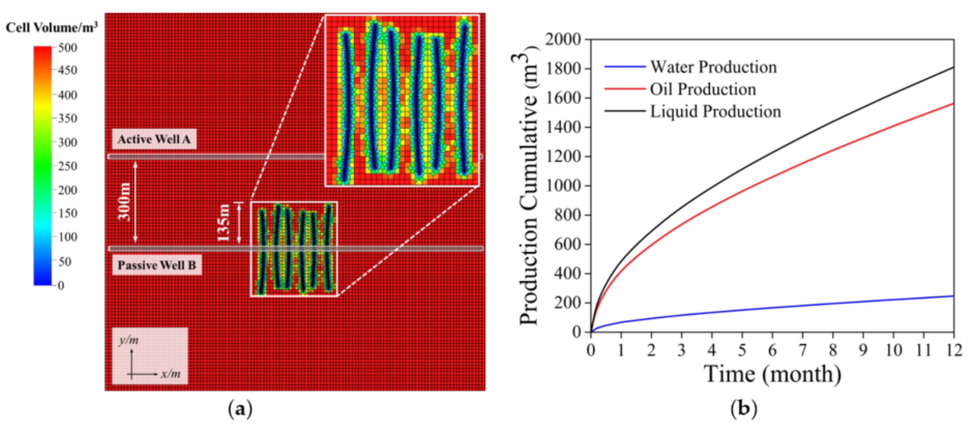
3.2.1. Model Construction

The base case of the multilayered UFM was constructed as a 1200 m × 1200 m × 32 m box, which was discretized into 120 × 120 × 7 grid blocks (Figure 7). Vertically, the model was divided into three layers that, from top to bottom, were 10 m, 12 m, and 10 m thick. The top and bottom layers represented the upper and lower barriers, respectively, while the middle layer represented the target formation. Two multi-fractured horizontal wells (passive well, active well) were situated in the middle layer, 200 m apart, with three respective perforation sections. Each section contained two perforation clusters that were spaced 40 m apart. The formation parameters used in this model are summarized in

Table 1. Base case formation parameters in the numerical simulations.

Parameters	Values
	Upper Barrier	Target Formation	Lower Barrier
Matrix density, kg/m3	2499	2499	2499
Reservoir depth, m	3092	3102	3114
Layer thickness, m	10	12	10
Porosity	0.01	0.09	0.01
Permeability, mD	0.01	1.5	0.01
Young’s modulus, GPa	30	25.7	30
Poisson’s ratio	0.3	0.21	0.3
Tensile strength, MPa	5	5	5
Initial reservoir pressure, MPa	38	38	38
Initial water saturation	0.9	0.43	0.9
Maximum horizontal stress, MPa	69	67	70
Minimum horizontal stress, MPa	54	52	55
Vertical stress, MPa	77	77	77

and were obtained from field data. Furthermore, a discrete fracture network (DFN) was integrated to characterize the NF system in the formation. The direction, coordinates, length, and mechanical properties of the NFs were based on the log interpretation data and drawn from the probability density function (

Table 2. Base case NF system parameters in the numerical simulations.

Parameters	Values
	Average	Std. Deviation
Fracture length, m	30	0
Intersection angle, °	40	10
Fracture density, m/m2	0.07	-
Friction coefficient	0.6	-
Cohesion, MPa	4	-

).

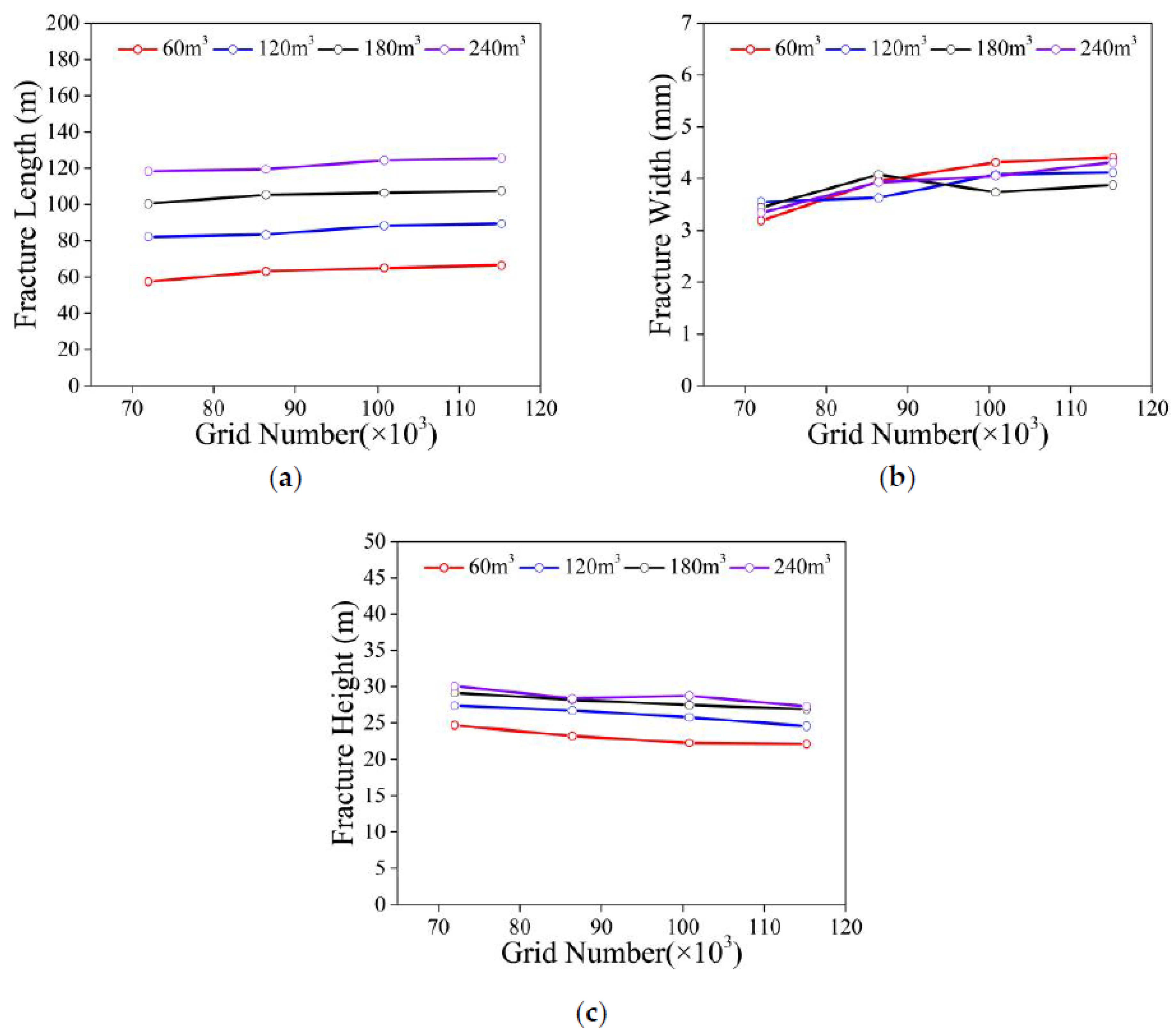
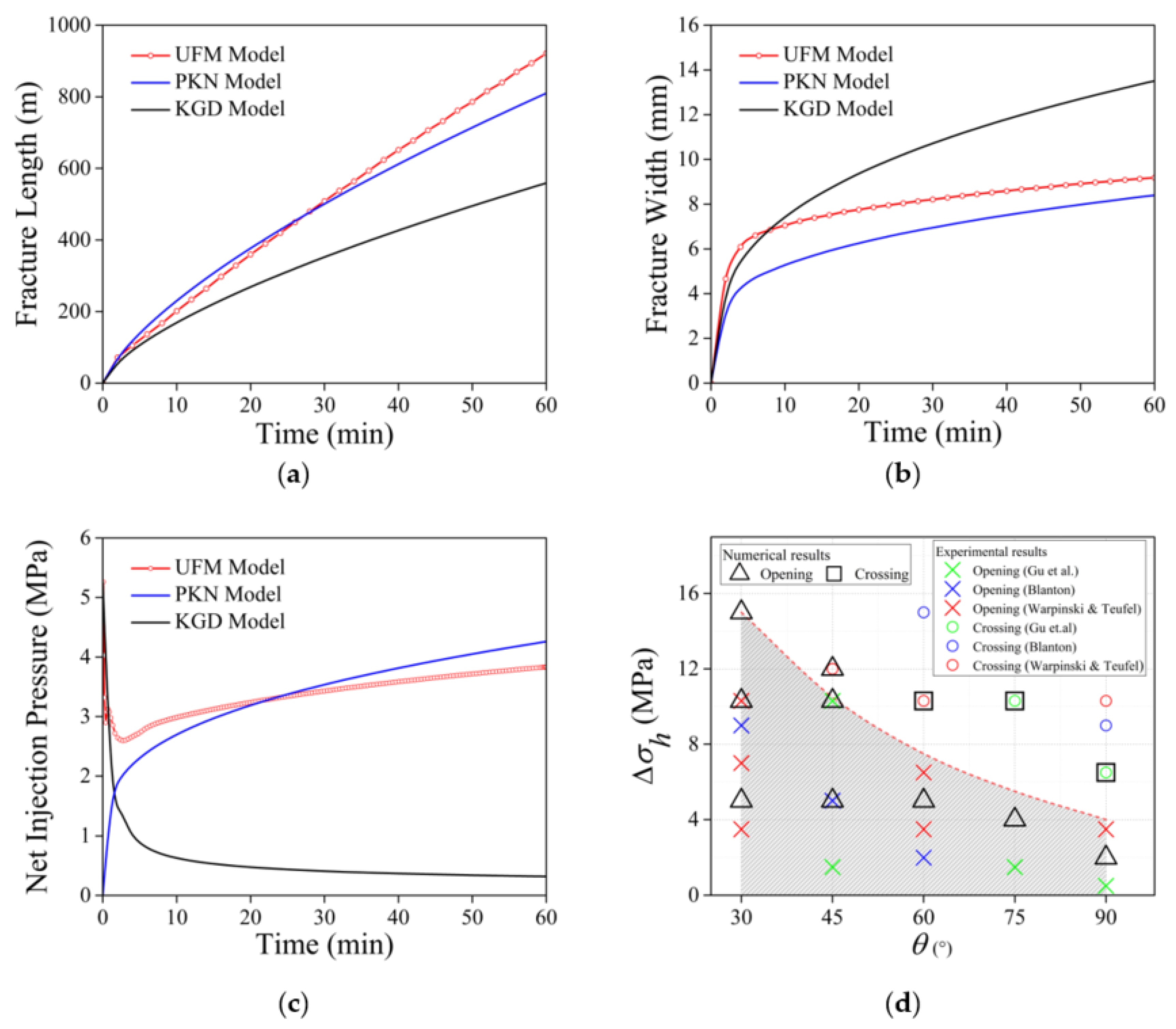
3.2.2. Model Verification

The numerical simulations in this research focus on the process of HF propagation. In recognition of the fact that the final accuracy of a numerical experiment is related to the grid quality, changes to the HF parameters (i.e., length, width, and height) were used as indicators for verifying grid independence. Specifically, four grid numbers—72,000, 86,400, 100,800, and 115,200—were designed to compare the changes in HF parameters under different volumes of injected fluid, i.e., 60 m³, 120 m³, 180 m³, and 240 m³. As shown in Figure 8, the values of HF parameters change very slightly as the number of grids increases from 100,800 to 115,200 under the same injected fluid volume. Therefore, the number of grids in the simulation model was set at 70,800 for this research, as illustrated in Figure 7b.

The reliability of using the UFM for bi-wing fractures was validated against experimental and numerical results from previous studies. To verify the accuracy of the UFM under target formation conditions, the UFM numerical results were first compared with analytical solutions using Perkins–Kern–Nordgren (PKN) and Khristianovich–Geertsma—Deklerk (KGD) models without leak-off. The primary formation parameters used for all the models are listed in Table 1. The input parameters consisted of liquid viscosity ($\mu$) and injection rate $(Q_t)$, which were 1 mPa·s and 3 m³/min, respectively.

The fracture length, width, and net injection pressure comparison results are shown in Figure 9a–c. In general, during the early stage of fracture propagation, the KGD model produces more accurate results than the PKN model. However, as the fracture grows longer, the PKN model results surpass those of the KGD model [40]. In this case, during the early stage, the numerical results are in agreement with the KGD model, but as time progresses, they tend to show a stronger correlation with the PKN model analytical solutions.

Moreover, to further evaluate the UMF’s numerical accuracy in simulating the HF–NF intersection process, a comparison case was designed in which two NFs were symmetrically distributed on the HF propagation path. A series of numerical simulations were then conducted and compared with published experimental results [39,41,42]. To approximate the conditions in the published experiments, the horizontal stress anisotropy $∆{\sigma }_h$ was set to 0~15 MPa ($∆{\sigma }_h={\sigma }_H-{\sigma }_h$) and the intersection angle $\theta$ equaled 0~90°. The NF properties that were used in all the numerical simulations are listed in Table 2. The simulation results are found in

Table 3. Numerical results at different $\theta$ and $∆{\sigma }_h$.

$\mathit{\theta } =35°$	$\mathit{\theta } =45°$	$\mathit{\theta } =60°$	$\mathit{\theta } =75°$	$\mathit{\theta } =90°$
		-	-	-

and summarized in Figure 9d. A comparison of the simulated and experimental results showed good agreement, and demonstrated some consistent patterns: (1) NFs are more likely to be opened by the HF when high-stress anisotropies and low-intersection angles are jointly present; and (2) the probabilities of the HF opening and crossing NFs are almost the same for the target formation, which increases the complexity of frac/frac connections between wells.

4. Results and Discussion

The impacts of various parameters, including horizontal stress distribution, anisotropies, and natural fracture density/orientation were individually investigated using the base model described in Figure 7. The primary properties used in the simulations are listed in Table 1 and Table 2. When there was a range of potential parameter values, (e.g., horizontal stress anisotropy ${\sigma }_H$ = 52~67 MPa, natural fracture density $\rho$= 0.06~0.13 m/m², intersection angle $\theta$= 0~50°, and perforation spacing $S$= 20~40 m), the influence of each parameter was determined. All other parameters remained constant. As per the fracturing pump schedules that are commonly used in stimulation operations, two kinds of fluids with different viscosities (3 mPa·s and 30 mPa·s) were pumped at a rate of $Q_t$= 5 m³/min.

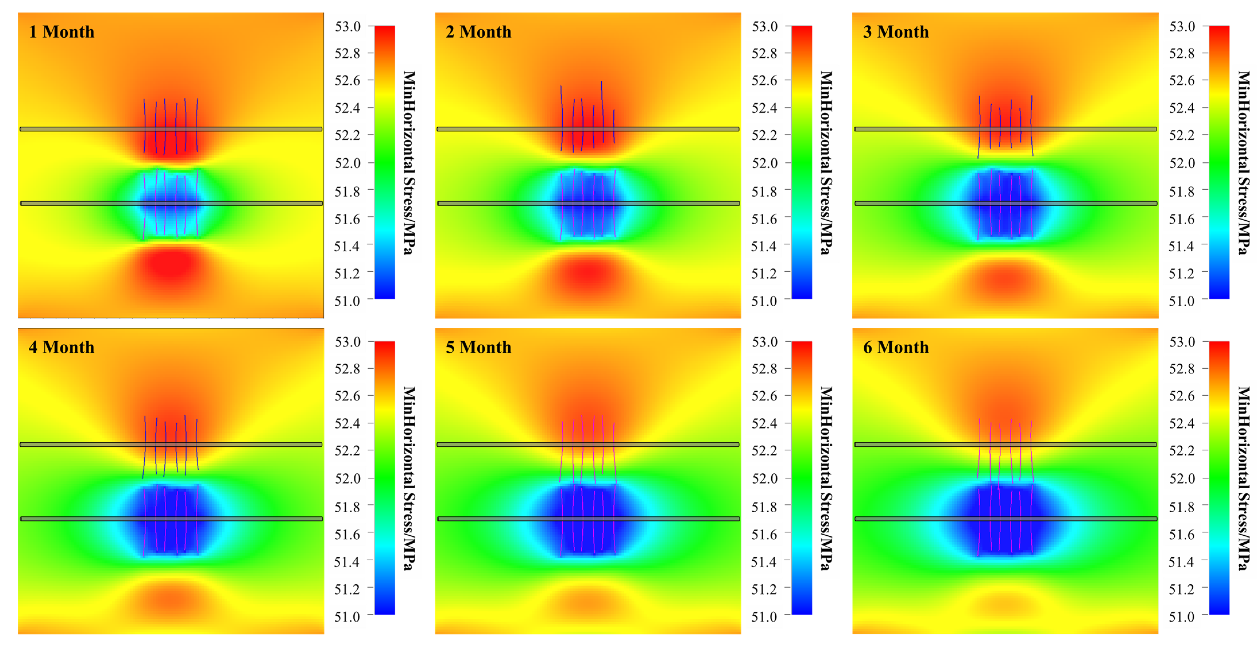
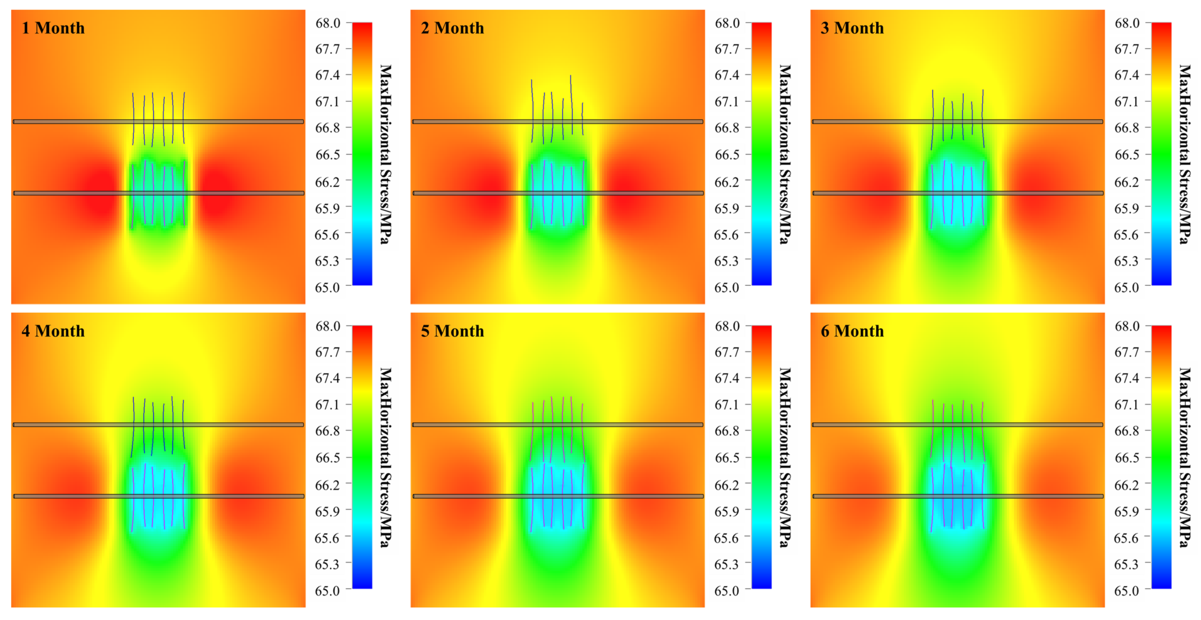
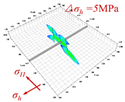
4.1. Horizontal Stress Distribution

Extensive field analyses have shown that the pressure depletion caused by production is one of the main factors facilitating well-to-well communication. Herein, the reservoir pressure distribution in passive well B’s drainage area was simulated. Subsequently, both its effect on the horizontal in-situ stress evolution, and Active Well A’s consequent fracture morphologies, were evaluated. All simulation cases were carried out according to the workflow described in Figure 4 and included the following steps: (1) the present fracture model was conducted in a limiting case, where the half-fracture length of passive well B was close to 135 m and the well spacing was 300 m; (2) automatic unstructured grid generation technology was used to set up the reservoir model (Figure 10a), which was validated with available field production data (Figure 10b) and employed to obtain the reservoir pressure distribution under different production times (Figure 11); (3) the geo-mechanical model was utilized to determine the evolution of the in-situ stress state, which was subsequently input as an initial condition to simulate the fracture propagation of Active Well A (Figure 12). In addition, these simulation cases neglected NFs in the formation to eliminate their impact. Finally, the volume of fluid injected into the perforation clusters equaled 1278 m³.

For the reservoir fluid outflow, the producer with the HFs (i.e., passive well B) created a depleted pressure zone which gradually expanded over time (Figure 11). In response, the horizontal in-situ stress in the drainage area decreased in parallel with the reservoir pressure (Figure 12 and Figure 13).

Mukherjee [12] characterized this change based on field data analysis, and the same features he reported were observed herein. It was noted that the depletion area exhibited a lower in-situ stress state, while the stress concentration outside this region was generated in a specific range due to deformation within the formation. For this reason, during the first two months of production, the HFs in adjacent Active Well A tended to propagate to the side, away from passive well B. An 8 MPa pressure drop was detected between the boundary and the center of this drainage area. Five months after the depleted pressure zone was created, it had spread to the perforation sections of adjacent Active Well A. Moreover, at this time, the horizontal stresses on both sides of Active Well A differed, and the horizontal stress on one side of passive well B was smaller than on the other. This stimulated the HF to extend towards the lower stress zone and caused the wing length ratio to exceed 1.6:1. Thus, by the fifth month after the depleted pressure zone was generated, the HFs between the wells were close to connecting. This connection finally occurred during the sixth month. These results demonstrated that the pressure depletion zone created by oil production is also a low-horizontal-stress area, which results in a nonuniform pressure distribution throughout the formation. Furthermore, the boundary of this pressure depletion zone continues to expand outward over time. When the outer boundary reaches the horizontal wellbore of the adjacent well, the HF’s two wings will be in different stress states. Consequently, less propagation energy for the wing in the low-stress area facilitates excessive growth towards the production well.

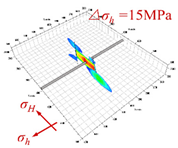
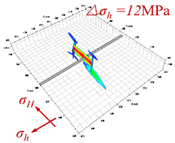
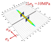
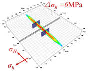
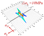
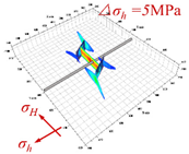
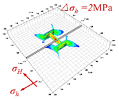
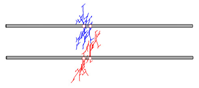
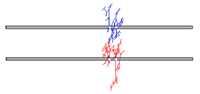
4.2. Horizontal Stress Anisotropies

The horizontal in-situ stress difference is one of the main factors affecting the HF network geometry. To investigate its influence, the fracture model simulation was outfitted with four horizontal stress anisotropies, where the minimum horizontal stress was 52 MPa and the maximum horizontal stresses were 52, 57, 62, and 67 MPa. The NF system exhibited a 0.07 m/m² linear density, which equaled the total length of all the NFs divided by the formation area. In each simulation case, the volume of injected liquid was adjusted to control the average length of the fracture network and ensure it was comparable throughout all four experiments (155.46, 154.73, 155.93, and 156.59 m), and also that it remained constant in every perforation cluster.

All the simulation results are illustrated in Figure 14. When $∆{\sigma }_h$= 0 MPa, the HFs tended to propagate along the NF paths, which implies that NFs exert significant control on HF geometries. Increasing the horizontal stress anisotropies ($∆{\sigma }_h$= 5, 10, and 15 MPa) reduced the complexity of the fracture network; the HF mainly grew in the direction of maximum horizontal stress. Thus, compared with the scenario in which $∆{\sigma }_h$= 0 MPa, the HF network became longer and narrower under higher horizontal stress anisotropy conditions. Furthermore, it should be noted that one wing of a HF will excessively propagate when the other wing is arrested by NFs. This aggravates the HF geometry asymmetry and increases the risk of frac/frac connections between wells. Moreover, the fluid pressure within the HF network increased as the $∆{\sigma }_h$ increased. Consequently, it can be surmised that high pressure frac-fluid will cause serious damage as HFs invade into adjacent wells.

The present findings confirm that lower horizontal stress anisotropies enhance the complexity of HF patterns and cause intra-well fractures to connect. When the horizontal stress anisotropy increases, the HF network becomes longer and narrower. When one wing of the HF might be arrested by the NF, the other wing will over-extend. Another issue that must be addressed is the fact that the amount of liquid injected into each fracture is not equal in most cases. Thus, an HF in a dominant position will excessively propagate and result in the connection of inter-well HFs.

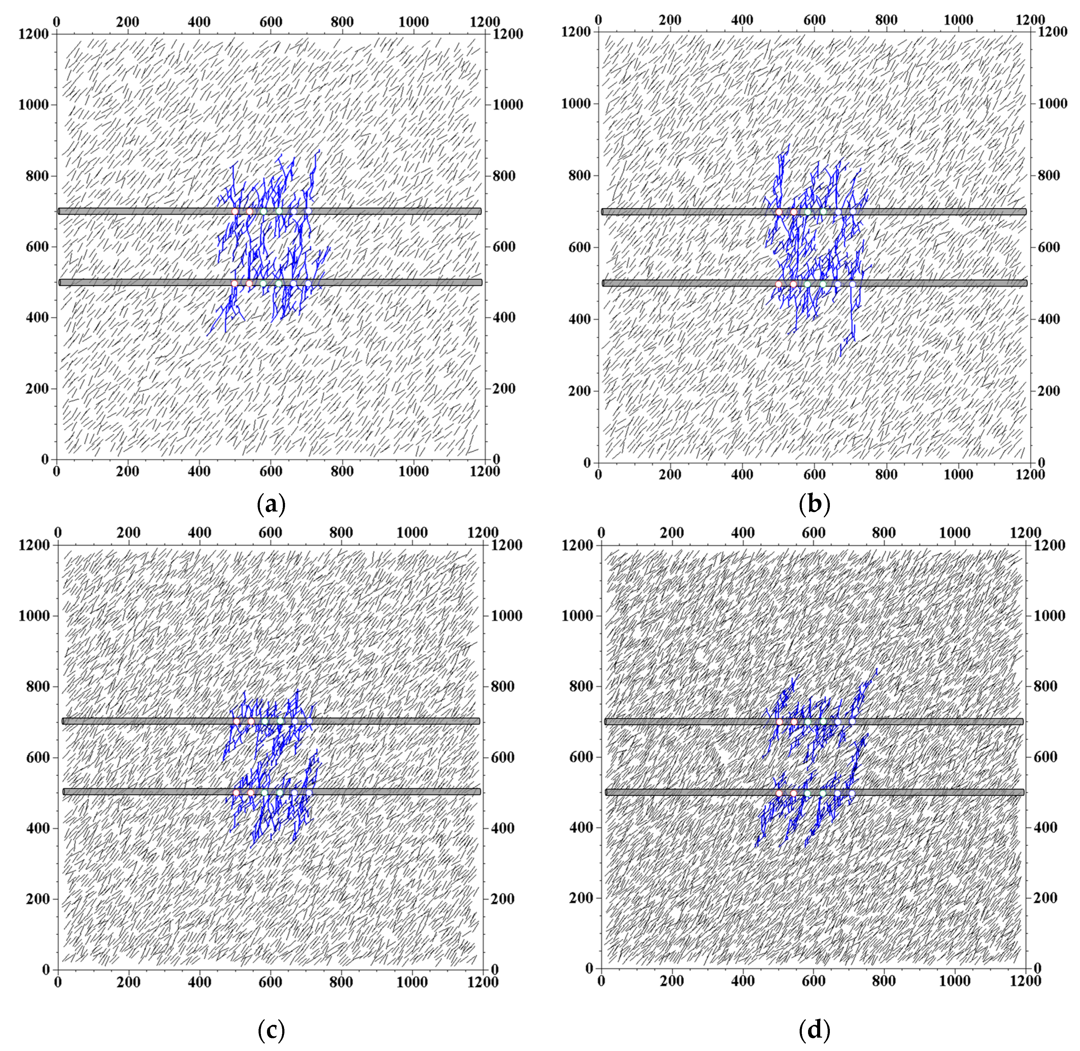
4.3. Natural Fracture Density

The fourth case showed frac/frac connections in the base model’s initial stress condition (${\sigma }_h$ = 52 MPa, ${\sigma }_H$ = 67 MPa). When testing this scenario, the liquid volume was first increased to ensure that all HFs between the two wells were connected. Subsequently, natural fractures of four different densities were selected in order to evaluate how the NF system affects the HF network geometry. The presence of inter-well communication was investigated at NF densities of 0.06, 0.07, 0.09, and 0.13 m/m².

Moreover, Figure 15 depicts the HF propagation results at all four NF densities. Under the same injection fluid volume, a smaller NF density (0.06, 0.07 m/m²) led to a longer fracture length and lower HF network complexity. As the NF density increased (0.09, 0.13 m/m²), the fracture length decreased and a complex HF network was formed near the well. The results from the inter-well fracture connection investigation in all the simulation cases are summarized in

Table 4. Inter-well frac/frac connections for different NF densities.

0.06 m/m2	0.07 m/m2	0.09 m/m2	0.013 m/m2
			None Connection
		-
		-

. In the cases where the NF density equaled 0.09 and 0.13 m/m², the NF’s control over the HF propagation path was enhanced and it deflected the fracture network towards the NF system (intersection angle $\theta$ = 30~50°). Furthermore, it was also observed that the inter-well HFs more easily connected under lower NF density (0.06, 0.07 m/m²) conditions.

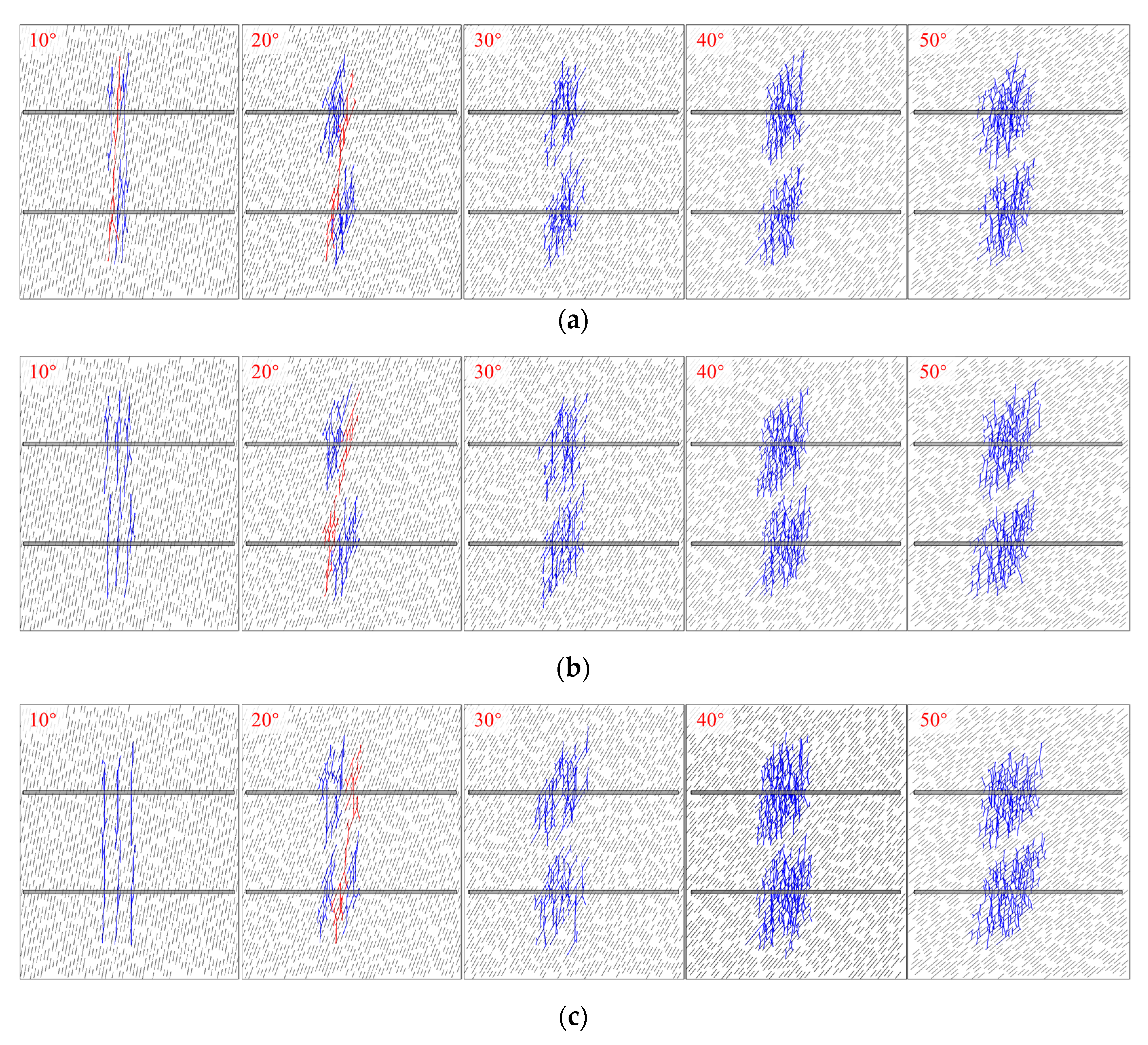
4.4. Natural Fracture Orientation

A thorough understanding of how the NF system affects the HF paths is important for predicting what shape the HF network will develop in response to multiple-fracture treatments. HF propagation along the NF path generates some offset along the x-axis, which may help to avoid frac/frac connections. Therefore, the HF growth path at various natural fracture orientations$—\alpha$ = 10, 20, 30, 40, and 50°—was also investigated. For this assessment, each well contained three fractures with initial fracture spacings of 20, 30, and 40 m, respectively. The NF fracture density was set to 0.07 m/m², the well spacing to 300 m, and the half length of each HF was controlled to 150 m, i.e., the critical condition for inter-well fracture connection. Finally, the NF orientation value $\alpha$ was set to the same values as the intersection angle $\theta$.

Figure 16 compares the HF network geometries from two wells with different fracture spacings and orientations. At smaller orientations ($\alpha$ = 10, 20°), the HFs mainly grew along the NF system path. Furthermore, a lateral offset of 20~30 m was generated, which resulted in the HFs deviating, yet the two wells were still able to connect. When the NF orientation was increased but the fracture spacing remained unchanged, the lateral offset increased, the inter-well fracture networks became staggered, and connection was avoided. Many previous experiments discussed above, along with the numerical simulation verification results presented herein (Figure 9d), indicate that a progressively larger intersection angle increases the ease with which the HFs can pass through the NFs. Taleghani [20] proposed and evaluated a mechanism for reinitiating fractures at the intersection of an HF and pre-existing NF. His numerical simulation results showed that when NFs in the formation are distributed at higher angles, a single HF can open the NF and continue to expand along its path during the propagation process under different stress differences. When the stress difference is high, however, and the HF has expanded to the end of the NF, it will either pass through the NF or rotate in the direction of maximum principal stress via a small turning angle. Moreover, the two wings that are formed in association with the HF are relatively symmetrical. For this reason, as the intersection angle increases ($\alpha$= 30, 40, 50°), the HF network shape becomes more complex and symmetrical. In general, the possibility of inter-well HF connection is small when the fracture spacing and intersection angle are high.

The extensive results laid out in Section 4.3 and 4.4 show some interesting facts. With respect to the pre-existing NF system, the HF path is more sensitive to density increases, while the asymmetric propagation shows some weakening at higher intersection angles. Furthermore, when the intersection angle is small, the use of larger fracture spacing can compel the HFs to stagger and thereby prevent any connection.

5. Conclusions

The type of FDI that interacts through conductive fracture pathways, resulting in more direct and greater damage to the older adjacent passive wells, is often associated with complex fracture-propagation patterns. In this work, the unconventional fracture model (UFM) is used for multi-stage, multi-cluster hydraulic fracturing simulations and includes an older adjacent passive well and an active well. Several important factors are considered in the numerical experiments, including horizontal stress distribution, horizontal stress anisotropies, NF density, and orientations. Some new mechanisms for inter-well HF connection at the interaction of HFs induced from different wells have been proposed.

The asymmetric propagation of HFs is the main problem associated with inter-well communication, where the evolution of horizontal in-situ stress and character parameters of NF systems in the formation both play a crucial role. The non-uniform distribution of horizontal in-situ stress resulting from pressure depletion strengthens the asymmetry of HF geometries. In addition, lower horizontal stress anisotropies enhance the complexity of HF patterns and make this problem more complicated. For the pre-existing NF system, the HF path is more sensitive as density increases, while the asymmetric propagation weakens with high intersection angles. These observations suggest important characteristics of the frac/frac connections between wells, which can be used to optimize fracture design and develop strategies for relevant measures to handle FDIs.

References

1. Ren, W.; Li, G.; Tian, S. Analytical modelling of hysteretic constitutive relations governing spontaneous imbibition of fracturing fluid in shale. J. Nat. Gas Sci. Eng. 2016, 34, 925–933. [Google Scholar] [CrossRef]
2. Daneshy, A.; George, K. Horizontal Well Frac-Driven Interactions: Types, Consequences, and Damage Mitigation. J. Pet. Technol. 2019, 71, 45–47. [Google Scholar] [CrossRef]
3. Merkle, S.; Lehmann, J.; James, P. Field Trial of a Cased Uncemented Multi-Fractured Horizontal Well in the Horn River. In Proceedings of the SPE/AAPG/SEG Unconventional Resources Technology Conference, Denver, CO, USA, 12–14 August 2013. [Google Scholar]
4. Sardinha, C.; Petr, C.; Lehmann, J.; James, P. Determining Interwell Connectivity and Reservoir Complexity through Frac Pressure Hits and Production Interference Analysis. In Proceedings of the SPE/CSUR Unconventional Resources Conference—Canada, Calgary, AB, Canada, 30 September–2 October 2014. [Google Scholar]
5. Tang, H.; Yan, B.; Chai, Z.; Zuo, L.; Killough, J.; Zhuang, S. Analyzing the Well-Interference Phenomenon in the Eagle Ford Shale/Austin Chalk Production System with a Comprehensive Compositional Reservoir Model. SPE Res. Reserv. Eval. Eng. 2019, 22, 827–841. [Google Scholar] [CrossRef]
6. Cao, R.; Li, R.; Girardi, A.; Chowdhury, N.; Chen, C. Well Interference and Optimum Well Spacing for Wolfcamp Development at Permian Basin. In Proceedings of the SPE/AAPG/SEG Unconventional Resources Technology Conference, Austin, TX, USA, 24–26 July 2017. [Google Scholar]
7. Pang, W.; Ehlig-Economides, C.A.; Du, J.; He, Y.; Zhang, T. Effect of Well Interference on Shale Gas Well SRV Interpretation. In Proceedings of the SPE Asia Pacific Unconventional Resources Conference and Exhibition, Brisbane, Australia, 9–11 November 2015. [Google Scholar]
8. Mohammad, R.; Gian, G.; Sathish, S.; Molinari, D. Automatic Well Interference Identification and Characterization: A Data-Driven approach to Improve Field Operation. In Proceedings of the SPE Annual Technical Conference and Exhibition, Calgary, AB, Canada, 30 September–2 October 2019. [Google Scholar]
9. Scott, E.; Young, S.; Ely, J.; Jones, D.; Vasquez, O. Lost in the Shadows: Surviving Fracturing Hazards with Fluid Tracking. In Proceedings of the SPE Hydraulic Fracturing Technology Conference and Exhibition, The Woodlands, TX, USA, 4–6 February 2020. [Google Scholar]
10. Sookprasong, P.A.; Hurt, R.S.; Gill, C.C. Downhole Monitoring of Multicluster, Multistage Horizontal Well Fracturing with Fiber Optic Distributed Acoustic Sensing (DAS) and Distributed Temperature Sensing (DTS). In Proceedings of the International Petroleum Technology Conference, Kuala Lumpur, Malaysia, 10–12 December 2014. [Google Scholar]
11. Roussel, N.P.; Agrawal, S. Introduction to Poroelastic Response Monitoring—Quantifying Hydraulic Fracture Geometry and SRV Permeability from Offset-Well Pressure Data. In Proceedings of the SPE/AAPG/SEG Unconventional Resources Technology Conference, Austin, TX, USA, 24–26 July 2017. [Google Scholar]
12. Mukherjee, H.; Poe, B.D.; Heidt, J.H.; Watson, T.B.; Barree, R.D. Effect of Pressure Depletion on Fracture-Geometry Evolution and Production Performance. SPE Prod. Facil. 2000, 15, 144–150. [Google Scholar] [CrossRef]
13. Manchanda, R.; Bhardwaj, P.; Hwang, J.; Sharma, M.M. Parent-Child Fracture Interference: Explanation and Mitigation of Child Well Underperformance. In Proceedings of the SPE Hydraulic Fracturing Technology Conference and Exhibition, The Woodlands, TX, USA, 23–35 January 2018. [Google Scholar]
14. Agrawal, S.; Sharma, M.M. Impact of Pore Pressure Depletion on Stress Reorientation and Its Implications on the Growth of Child Well Fractures. In Proceedings of the SPE/AAPG/SEG Unconventional Resources Technology Conference, Houston, TX, USA, 23–35 July 2018. [Google Scholar]
15. Taherdangkoo, R.; Tatomir, A.; Anighoro, T. Modeling fate and transport of hydraulic fracturing fluid in the presence of abandoned wells. J. Contam. Hydrol. 2019, 221, 58–68. [Google Scholar] [CrossRef] [PubMed]
16. Tatomir, A.; Mcdermott, C.; Bensabat, J. Conceptual model development using a generic Features, Events, and Processes (FEP) database for assessing the potential impact of hydraulic fracturing on groundwater aquifers. J. Adv. Geosci. 2018, 45, 185–192. [Google Scholar] [CrossRef] [Green Version]
17. Guo, X.; Wu, K.; Killough, J.; Tang, J. Understanding the Mechanism of Interwell Fracturing Interference with Reservoir/Geomechanics/Fracturing Modeling in Eagle Ford Shale. SPE Reserv. Eval. Eng. 2019, 22, 842–860. [Google Scholar] [CrossRef]
18. King, G.E.; Rainbolt, M.F.; Swanson, S. Frac Hit Induced Production Losses: Evaluating Root Causes, Damage Location, Possible Prevention Methods and Success of Remedial Treatments. In Proceedings of the SPE Annual Technical Conference and Exhibition, San Antonio, TX, USA, 9–11 October 2017. [Google Scholar]
19. Olson, J.E.; Taleghani, A.D. Modeling simultaneous growth of multiple hydraulic fractures and their interaction with natural fractures. In Proceedings of the SPE Hydraulic Fracturing Technology Conference, The Woodlands, TX, USA, 19–21 January 2009. [Google Scholar]
20. Taleghani, A.D. Fracture Re-Initiation as a Possible Branching Mechanism During Hydraulic Fracturing. In Proceedings of the 44th U.S. Rock Mechanics Symposium and 5th U.S.-Canada Rock Mechanics Symposium, Salt Lake City, UT, USA, 27–30 June 2010. [Google Scholar]
21. Sesetty, V.; Ghassemi, A. Simulation of Hydraulic Fractures and Their Interactions with Natural Fractures. In Proceedings of the 46th U.S. Rock Mechanics/Geomechanics Symposium, Chicago, IL, USA, 24–27 June 2012. [Google Scholar]
22. Settgast, R.R.; Izadi, G.; Hurt, R.S.; Jo, H.; Johnson, S.M.; Walsh, S.C.; Moos, D.; Ryerson, F. Optimized Cluster Design in Hydraulic Fracture Stimulation. In Proceedings of the SPE/AAPG/SEG Unconventional Resources Technology Conference, San Antonio, TX, USA, 20–22 July 2015. [Google Scholar]
23. Duan, K.; Kwok, C.; Zhang, Q. On the initiation, propagation and reorientation of simultaneously-induced multiple hydraulic fractures. Comput. Geotech. 2020, 117, 103226. [Google Scholar] [CrossRef]
24. Malhotra, S.; Lehman, E.R.; Sharma, M.M. Proppant Placement Using Alternate-Slug Fracturing. SPE J. 2014, 19, 974–985. [Google Scholar] [CrossRef]
25. Ribeiro, L.H.; Sharma, M.M. A New Three-Dimensional, Compositional, Model for Hydraulic Fracturing with Energized Fluids. In Proceedings of the SPE Annual Technical Conference and Exhibition, San Antonio, TX, USA, 8–10 October 2012. [Google Scholar]
26. Ajani, A.; Mohan, K. Interference Study in Shale Plays. In Proceedings of the SPE Hydraulic Fracturing Technology Conference, The Woodlands, TX, USA, 6–8 February 2012. [Google Scholar]
27. Kurtoglu, B.; Salman, A. How to Utilize Hydraulic Fracture Interference to Improve Unconventional Development. In Proceedings of the Abu Dhabi International Petroleum Exhibition and Conference, Abu Dhabi, United Arab Emirates, 9–12 November 2015. [Google Scholar]
28. Yadav, H.; Motealleh, S. Improving Quantitative Analysis of Frac-Hits and Refracs in Unconventional Plays Using RTA. In Proceedings of the SPE Hydraulic Fracturing Technology Conference, The Woodlands, TX, USA, 24–26 January 2017. [Google Scholar]
29. Song, B.; Christine, E. Rate-Normalized Pressure Analysis for Determination of Shale Gas Well Performance. In Proceedings of the North American Unconventional Gas Conference and Exhibition, The Woodlands, TX, USA, 14–16 June 2011. [Google Scholar]
30. Weng, X.; Kresse, O.; Cohen, C.; Wu, R.; Gu, H. Modeling of Hydraulic-Fracture-Network Propagation in a Naturally Fractured Formation. SPE Prod. Oper. 2011, 26, 368–380. [Google Scholar]
31. Kresse, O.; Weng, X. Numerical Modeling of Hydraulic Fractures Interaction in Complex Naturally Fractured Formations. Rock Mech. Rock Eng. 2013, 46, 555–568. [Google Scholar] [CrossRef]
32. Liu, H.; Luo, Y.; Zhang, N. Unlock Shale Oil Reserves Using Advanced Fracturing Techniques: A Case Study in China. In Proceedings of the International Petroleum Technology Conference, Beijing, China, 26–28 March 2013. [Google Scholar]
33. Matteo, M.; Lee, D.; Dan, S.; Morales, A. Advanced Modeling of Interwell-Fracturing Interference: An Eagle Ford Shale-Oil Study. J. Pet. Sci. Eng. 2016, 21, 1567–1582. [Google Scholar]
34. Fung, R.L.; Vilayakumar, S.; Cormack, D.E. Calculation of Vertical Fracture Containment in Layered Formations. SPE Form. Eval. 1987, 2, 518–522. [Google Scholar] [CrossRef]
35. Cohen, C.; Kresse, O.; Weng, X. Stacked Height Model to Improve Fracture Height Growth Prediction, and Simulate Interactions with Multi-Layer DFNs and Ledges at Weak Zone Interfaces. In Proceedings of the SPE Hydraulic Fracturing Technology Conference and Exhibition, The Woodlands, TX, USA, 24–26 January 2017. [Google Scholar]
36. Morales, A.; Zhang, K.; Gakhar, K. Advanced Modeling of Interwell Fracturing Interference: An Eagle Ford Shale Oil Study—Refracturing. In Proceedings of the SPE Hydraulic Fracturing Technology Conference, The Woodlands, TX, USA, 9–11 February 2016. [Google Scholar]
37. Ching, H.Y.; Weng, X.W. Mechanics of Hydraulic Fracturing, 2nd ed.; Gulf Professional Publishing: Houston, TX, USA, 2015; pp. 49–68. [Google Scholar]
38. Renshaw, C.E.; Pollard, D.D. An experimentally verified criterion for propagation across unbounded frictional interfaces in brittle, linear elastic materials. Int. J. Rock Mech. Min. Sci. Geomech. Abstr. 1995, 32, 237–249. [Google Scholar] [CrossRef]
39. Gu, H.; Weng, X.; Lund, J. Hydraulic Fracture Crossing Natural Fracture at Nonorthogonal Angles: A Criterion and Its Validation. SPE Prod. Oper. 2012, 27, 20–26. [Google Scholar] [CrossRef]
40. Wu, K.; Olson, J.E. Simultaneous Multifracture Treatments: Fully Coupled Fluid Flow and Fracture Mechanics for Horizontal Wells. SPE J. 2015, 20, 337–346. [Google Scholar] [CrossRef]
41. Warpinski, N.R.; Teufel, L.W. Influence of Geologic Discontinuities on Hydraulic Fracture Propagation (includes associated papers 17011 and 17074). J. Pet. Technol. 1987, 39, 209–220. [Google Scholar] [CrossRef]
42. Blanton, T.L. Propagation of Hydraulically and Dynamically Induced Fractures in Naturally Fractured Reservoirs. In Proceedings of the SPE Unconventional Gas Technology Symposium, Louisville, KY, USA, 18–21 May 1986. [Google Scholar]
Figure 1. (a) Type log for the Triassic Baikouquan formation of Mahu 131 block; (b) mineral composition statistics.
Energies 14 04881 g001
Figure 2. Typical responses of active/passive wells to FDIs in the Mahu 131 block.
Energies 14 04881 g002
Figure 3. Historical comparison of passive well A and a log–log plot of RNP vs. tMB during the two corresponding periods.
Energies 14 04881 g003
Figure 4. (a) Simplified complex hydraulic fracture/reservoir geomechanics modeling workflow; (b) expanded workflow used to model parent/child well fracture interference.
Energies 14 04881 g004
Figure 5. (a) Difference between a pseudo-3D model and planar-3D model (Cohen et al., 2017); (b) diagram depicting hydraulic and pre-existing natural fractures.
Energies 14 04881 g005
Figure 6. Schematic of a hydraulic fracture (HF) approaching a natural fracture (NF).
Energies 14 04881 g006
Figure 7. Construction of the base model for numerical simulations: (a) top view; (b) 3D view.
Energies 14 04881 g007
Figure 8. Results of grid independence verification. The changes to HF parameters, (a) fracture length, (b) fracture width, and (c) fracture height, under different volumes of injected fluid, i.e., 60 m3, 120 m3, 180 m3, and 240 m3.
Energies 14 04881 g008
Figure 9. Comparison between the UFM model and the PKN/KGD models for a bi-wing HF, and experiments for the HF–NF interaction: (a) fracture length vs. time curves; (b) fracture width vs. time curves; (c) net injection pressure vs. time curves; (d) the HF crossing or opening the NFs at different θ and σ h .
Energies 14 04881 g009
Figure 10. (a) Unstructured grid of the fractured reservoir model; (b) Production cumulative profile of the passive well.
Energies 14 04881 g010
Figure 11. Reservoir pressure variation at different production times.
Energies 14 04881 g011
Figure 12. Minimum horizontal in-situ stress distribution and fracture morphology at different production times under the impact of pressure depletion.
Energies 14 04881 g012
Figure 13. Maximum horizontal in-situ stress distribution and fracture morphology at different production times under the influence of pressure depletion.
Energies 14 04881 g013
Figure 14. HF geometries for different horizontal stress anisotropies: (a) σ h   = 0 MPa; (b) σ h   = 5 MPa; (c) σ h   = 10 MPa; (d) σ h   = 15 MPa.
Energies 14 04881 g014aEnergies 14 04881 g014b
Figure 15. HF geometries for different NF densities: (a) 0.06 m/m2; (b) 0.07 m/m2; (c) 0.09 m/m2; (d) 0.13 m/m2.
Energies 14 04881 g015
Figure 16. HF geometries for different NF orientations at varied fracture spacings: (a) 20 m; (b) 30 m; (c) 40 m.
Energies 14 04881 g016