A Hierarchical Control Approach for Power Loss Minimization and Optimal Power Flow within a Meshed DC Microgrid

Abstract

This work considers the DC part of a hybrid AC/DC microgrid with a meshed topology. We address cost minimization, battery scheduling and the power loss minimization within the power distribution network through constrained optimization. The novelty comes from applying differential flatness properties to the microgrid components and formulating the cost and constraints in terms of the associated B-splines parametrization of the flat outputs (the voltages and currents of the system). This allows us to obtain optimal power profiles to minimize the power dissipation and the cost of the electricity purchase from the external grid. These profiles are tracked by a model predictive controller at the higher level, while at a a lower level a controller deals with the operation of the switches within the DC/DC converters. Extensive simulations under nominal and fault-affected scenarios using realistic data validate the proposed approach.

1. Introduction

Microgrids are complex power systems and their efficient operation demands the study on multiple interlocking factors [1], such as power losses, electricity cost, renewable resources, component size and the like. To date, the state of the art in the microgrid topic has shown promising results in the power flow amelioration and performance enhancement [2]. Optimal power flow accounts for the effective and reliable functioning of the system by either minimizing the electricity cost or the energy dissipation. The existence of power loss in the transmission lines can greatly affect the quality of the power distribution. Therefore, the minimization of the power loss constitute a significant factor and leads towards the improvement of the power transmission [3].

Several techniques have been considered recently for the minimization of the power dissipation, emphasizing either the components linked to the microgrid or the transmission-line network [4]. For instance,

Refs. [5,6] focus on the the energy storage (ES) scheduling in combination with the use of renewable sources and their topology within the network. In other works, the researchers seek to reduce the existing power losses which exist in the transmission lines and cannot be avoided or ignored [7]. In the literature, researchers have proposed several methods for optimal power distribution including power loss minimization. In [8], a hierarchical control strategy divided into three levels is proposed to handle the energy management in stand-alone microgrids. More specifically, at the higher level, taking into account topological and stability issues, optimal power profiles are generated, within a MPC framework. At the middle level, using the upper level references, a voltage regulation problem is solved taking into account the power losses of the transmission network and the converters. Furthermore, a two-level hierarchical control based on plug and play method has been proposed in [9] where at a low level load sharing is achieved through droop control and at a higher level adaptive droop controllers are developed for power losses minimization. Ref. [10] introduces an optimal power flow algorithm for islanded microgrids to cope with central power dissipation under a centralized three-layer supervision controller.

In the literature and, in particular, in the references already mentioned, the dynamical models are usually taken into account as a group of differential equations without thoroughly representing and studying the power conservation among the components of the system. Regarding the optimal profiles, optimization control methods under constraints are employed using MPC to generate online optimal profiles for discrete time systems penalizing simultaneously the dissipation, the cost and the error that exist among the real and reference profiles. To the best of our knowledge only few works [4,5,6,7,8,9,10,11] deal specifically with the power dissipation issues. The strength of our work is related to the fact that it handles in a multi-objective optimization-based approach both optimal energy management and power losses minimization while satisfying constraints, rejecting disturbances and grasping the system’s multi-timescale characteristics.

Contributions: In [12], the complete three-layer hierarchical control strategy was presented. A constrained optimization-based problem was implemented in the absence of the power losses in the transmission-line network. In this paper, we further develop the optimization problem, particularly of the high level, already presented in [12], taking into account the power dissipation. In the following, we summarize the contributions of this work:

• Reduction in the power losses existing in the transmission lines is further added to the optimization to enhance the power flow while considering at the same time the cost reduction in the power consumption. The formulation of the high level optimization problem is done through the analytical computation of the system’s flat representation together with B-spline parametrization;
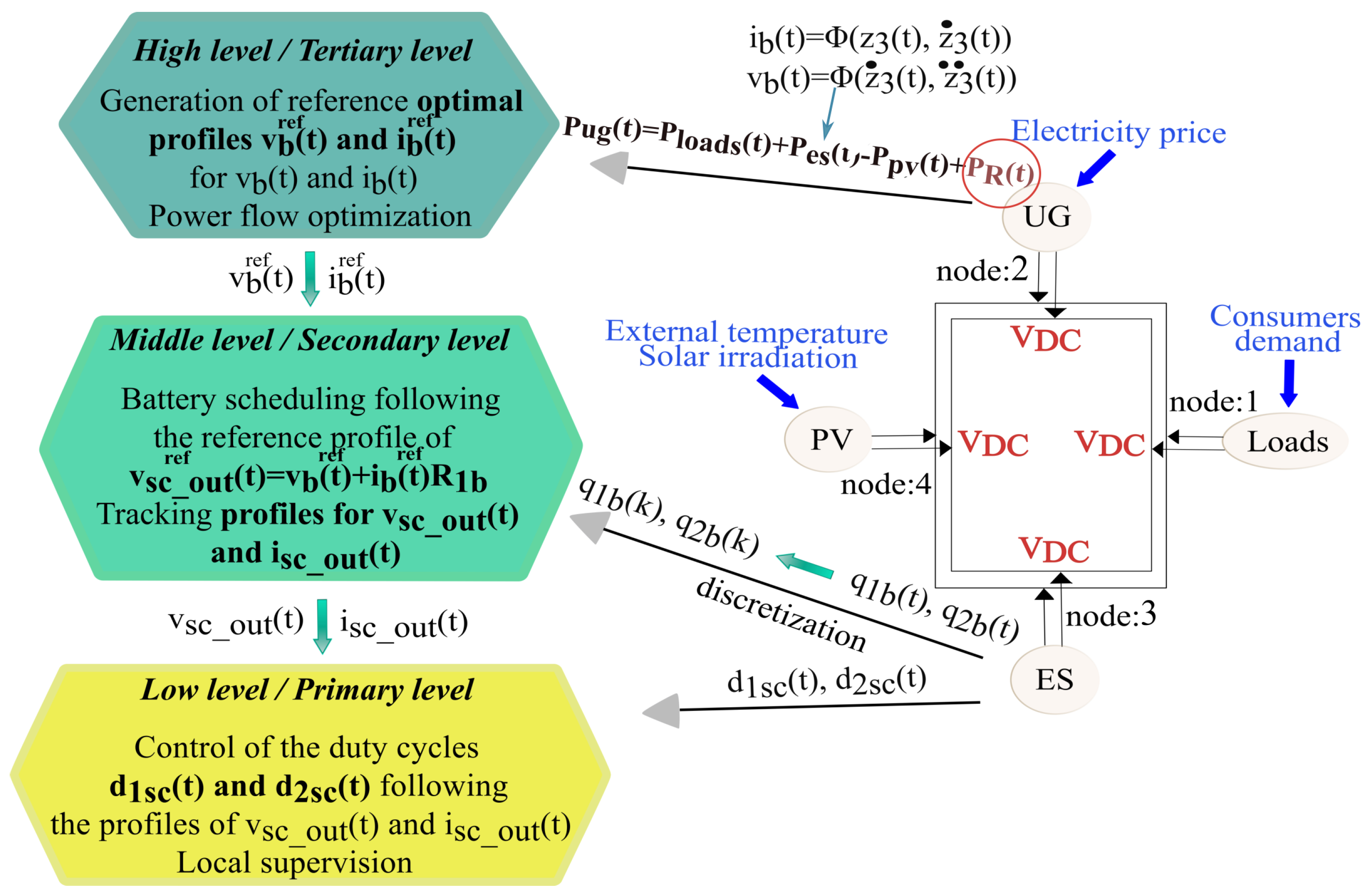
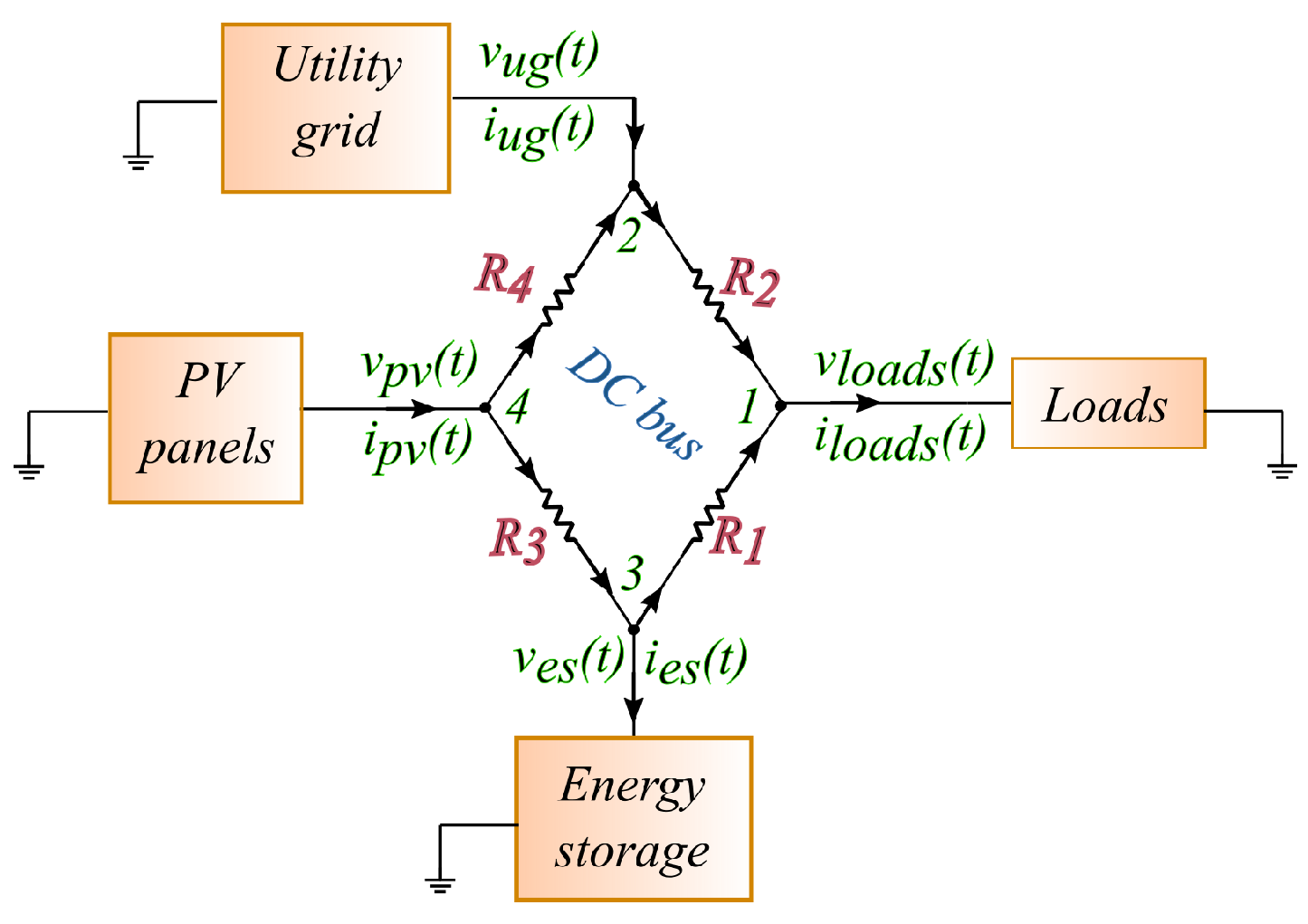
• Thorough presentation of the central transmission network describing in detail its dynamical model. The power dissipation is considered through the voltage drops among the four connecting nodes n: $1,2,3,4$ [13], illustrated in Figure 1 and the corresponding transmission lines are represented through four resistances, $R_{1,2,3,4}$. Additional constraints are taken into consideration to preserve the DC voltage close to the reference equal to 400 V;
• Verification of the meshed topology of the central network in the case of unexpected events (e.g., blackouts).

Note that the objective function will be posed in a flat representation (rewritten in terms of a flat output and its derivatives). Likewise will be done for the constraints. Further parametrizing the flat output by a family of B-spline functions will allow to check continuous time constraints. More details on the concepts of flatness and B-spline parametrization can be found in [14,15,16].

Outline:Section 2 concerns the abbreviations. In Section 3 a brief description of the ES (Energy Storage) dynamics is introduced and the detailed model of the central transmission network are introduced. Section 4 contains the multilevel hierarchical control problem, with the high and the middle levels being detailed in particular. The results are introduced in Section 5. Finally, Section 6 presents the outcomes of this work.

2. Notations

$ES,es$	energy storage system
$UG,ug$	utility grid
$PV,pv$	solar panel system
$DERs$	distributed energy resources
$x\left(t\right)$	state vector of the system $\in R^n$
$u\left(t\right)$	input vector of the system $\in R^m$
$y\left(t\right)$	output vector of the system $\in R^m$
n	connecting node between a source or a load and the DC-bus
$KiBaM$	Kinetic Battery Model
P	electrical power
$Sw$	switch of the DC/DC converter
$d_{1sc},d_{2sc}$	duty cycles of the switches within the Split Pi converter
$q_{1b},q_{2b}$	available and bound charge of the KiBaM battery
b	KiBaM battery
$sc$	Split−Pi Converter
C	capacitor
I	inductor
$R_{1b}$	resistance between the KiBaM battery and the Split−Pi
$\phantom{.}$	converter
$R_{2b}$	resistance of the KiBaM battery
$R_1,\phantom{.}{R}_2,\phantom{.}{R}_3,\phantom{.}{R}_4$	resistances of the transmission network
$R_{1sc}$	resistance among the DC network and the Split−Pi
$\phantom{.}$	converters
$i_{sc\_out}$	output current of the Split−Pi converter
$v_{sc\_out}$	output voltage of the Split−Pi converter
$i_{sc\_in}$	input current of the Split−Pi converter
$v_{sc\_in}$	input voltage of the Split−Pi converter
r	derivative of the B-spline
$p_i$	$i^{}$th control point
$b_{i,d}$	$i^{}$th B-spline of order d
$\mathcal{B}\left(t\right)$	vector of the B-splines $\in R^{d\times N}$
$\mathcal{P}$	vector of control points $\in R^{3\times N}$
${\mathcal{S}}_{\kappa ,d-r,d}$	translation matrix from higher to lower degree basis
$\phantom{.}$	functions
${\mathcal{M}}_{d,d-r}$	matrix performing the linear combinations of the
$\phantom{.}$	lower-degree basis functions
T	knot vector $\in R^{N+d}$
${\tau }_{\kappa }$	${\kappa }^{}$th knot
$\kappa$	number of knots
e	electricity price
$Q_{\tilde{y}},\phantom{.}{R}_{\tilde{u}}$	weight matrices

3. DC Microgrid Model Description

The DC microgrid, part of a hybrid AC/DC architecture with a meshed topology (Figure 1), considered in this work is also described in [12] and is composed by a set of PVs, an ES composed by lead acid batteries and a set of loads. These components are linked to the central transmission network (around 400 V DC) through a particular type of DC/DC converters: Split-Pi converters, which regulate the input/output voltage from and towards the sources and the loads. The DC microgrid is connected to the UG through an AC/DC converter. In this work, we analyze the dynamical model of the DC-bus together with the ES system (Split-Pi converter connected to the battery). However, the following approach can be similarly applied for the primarily proposed design in [17]. The overall hybrid AC/DC grid contains an AC/DC converter, placed between the grid and the DC microgrid (Figure 1), where supplementary buses (AC or DC) or sources (AC or DC) could be included, since a meshed topology of a multiple-line transmission network is considered. However, for an AC/DC converter, an AC bus or an AC source, the characteristics of the AC power should be taken into account, such as the active power, the reactive power, the frequency and the like [18].

This section builds upon our previous paper [12], where the mathematical model of the ES system was explicitly introduced. In this work, we will continue with the explicit description of the dynamics of the central transmission network, since the power losses are now considered and resistors exist to replace every transmission line. The mathematical methodology employed relies upon the PH formalism [19]. This method provides an explicit description of the routing elements (inductors, capacitors, resistors) existing in the electrical network. An advantage of this method is that the set of equations can be directly derived by the associated Bond Graph of the electrical system [20,21], which is a graph-oriented modeling tool for the dynamics of convoluted physical systems. The modeling methodology are thoroughly presented and analyzed in [12,17].

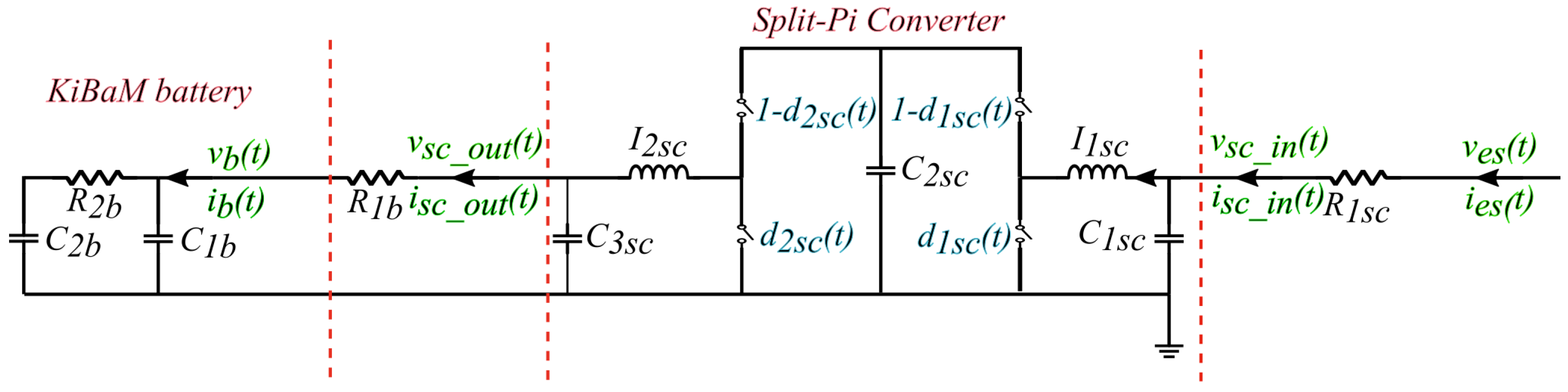
3.1. Brief Description of the ES Subsystem

The ES constitutes the Split-Pi converter connected to the battery as in Figure 2. The circuit of the battery is structured according to the Kinetic Battery Model (KiBaM), consisting of two capacitors and a resistance between them. The charges of the capacitors represent the total charge of the battery. Concerning the Split-Pi converter, it is a bidirectional buck-boost converter able to regulate the voltage in both directions.

The state-space representation of the ES system was already explicitly presented in [12] concluding to the following nonlinear state-space mathematical model:

$$\begin{array}{cc}\hfill {\dot{p}}_{1sc}\left(t\right)& ={\displaystyle \frac{q_{1sc}\left(t\right)}{C_{1sc}}}-{\displaystyle \frac{q_{2sc}\left(t\right)}{C_{2sc}}}(1-d_{1sc}\left(t\right)),\hfill \end{array}$$

(1a)

$$\begin{array}{cc}\hfill {\dot{p}}_{2sc}\left(t\right)& ={\displaystyle \frac{q_{2sc}\left(t\right)}{C_{2sc}}}(1-d_{2sc}\left(t\right))-{\displaystyle \frac{q_{3sc}\left(t\right)}{C_{3sc}}},\hfill \end{array}$$

(1b)

$$\begin{array}{cc}\hfill {\dot{q}}_{1sc}\left(t\right)& ={\displaystyle \frac{v_{DC}}{R_{1sc}}}-{\displaystyle \frac{q_{1sc}\left(t\right)}{C_{2sc}{R}_{1sc}}}-{\displaystyle \frac{p_{1sc}\left(t\right)}{I_{1sc}}},\hfill \end{array}$$

(1c)

$$\begin{array}{cc}\hfill {\dot{q}}_{2sc}\left(t\right)& ={\displaystyle \frac{p_{1sc}\left(t\right)}{I_{1sc}}}(1-d_{1sc}\left(t\right))-{\displaystyle \frac{p_{2sc}\left(t\right)}{I_{2sc}}}(1-d_{2sc}\left(t\right)),\hfill \end{array}$$

(1d)

$$\begin{array}{cc}\hfill {\dot{q}}_{3sc}\left(t\right)& ={\displaystyle \frac{p_{2sc}\left(t\right)}{I_{2sc}}}-i_{R_{1b}}\left(t\right),\hfill \end{array}$$

(1e)

$$\begin{array}{cc}\hfill {\dot{q}}_{1b}\left(t\right)& =i_{R_{1b}}\left(t\right)-{\displaystyle \frac{q_{1b}\left(t\right)}{C_{1b}{R}_{2b}}}+{\displaystyle \frac{q_{2b}\left(t\right)}{C_{2b}{R}_{2b}}},\hfill \end{array}$$

(1f)

$$\begin{array}{cc}\hfill {\dot{q}}_{2b}\left(t\right)& ={\displaystyle \frac{q_{1b}\left(t\right)}{C_{1b}{R}_{2b}}}-{\displaystyle \frac{q_{2b}\left(t\right)}{C_{2b}{R}_{2b}}}.\hfill \end{array}$$

(1g)

The p and q variables correspond to the magnetic flux of the inductors and the charges of the capacitors, respectively. These variables ($p_{1sc,2sc}$, $q_{1sc,2sc,3sc}$) structure the state vector of the ES system, $x_{es}$$\in R^{7\times 1}$. Next, $v_{DC}$ and $i_{R_{1b}}$ form the input vector $u_{es}$$\in R^{2\times 1}$ of the ES and $i_{DC}$ and $v_{R_{1b}}$ form the output vector $y_{es}$$\in R^{1\times 2}$. The circuit’s parameters are $I_{1sc}$, $I_{2sc}$, $C_{1sc}$, $C_{2sc}$, $C_{3sc}$, $C_{1b}$, $C_{2b}$, with I denoting the inductance of the inductor and C the capacitance of the capacitor. The state vector, the input vector and the output vector of the system are given analytically in [12]. Furthermore, from the ES circuit in Figure 2 and [12], we have the following relation which will be useful later in the energy management:

$$\begin{array}{cc}\hfill i_b\left(t\right)=& i_{R_{1b}}\left(t\right),\hfill \end{array}$$

(2a)

$$\begin{array}{cc}\hfill v_b\left(t\right)=& {\displaystyle \frac{q_{1b}\left(t\right)}{C_{1b}}}.\hfill \end{array}$$

(2b)

The Split-Pi converter is considered as an ideal one ( see also [13]), that is, the following relation is satisfied: $P_{sc\_in}=P_{sc\_out}$. Ohm’s law is taken into account to link the input and output voltage and current of the Split-Pi converter as in [12,13]. Hence, the ES power is given as in [13]: $P_{es}\left(t\right)=v_{es}\left(t\right)i_{es}\left(t\right)=(v_b\left(t\right)+i_b\left(t\right)R_{1b})i_b\left(t\right)+R_{1sc}{\left(\alpha \left(t\right)i_b\left(t\right)\right)}^2$ and will be used in the analysis and calculation of the cost function.

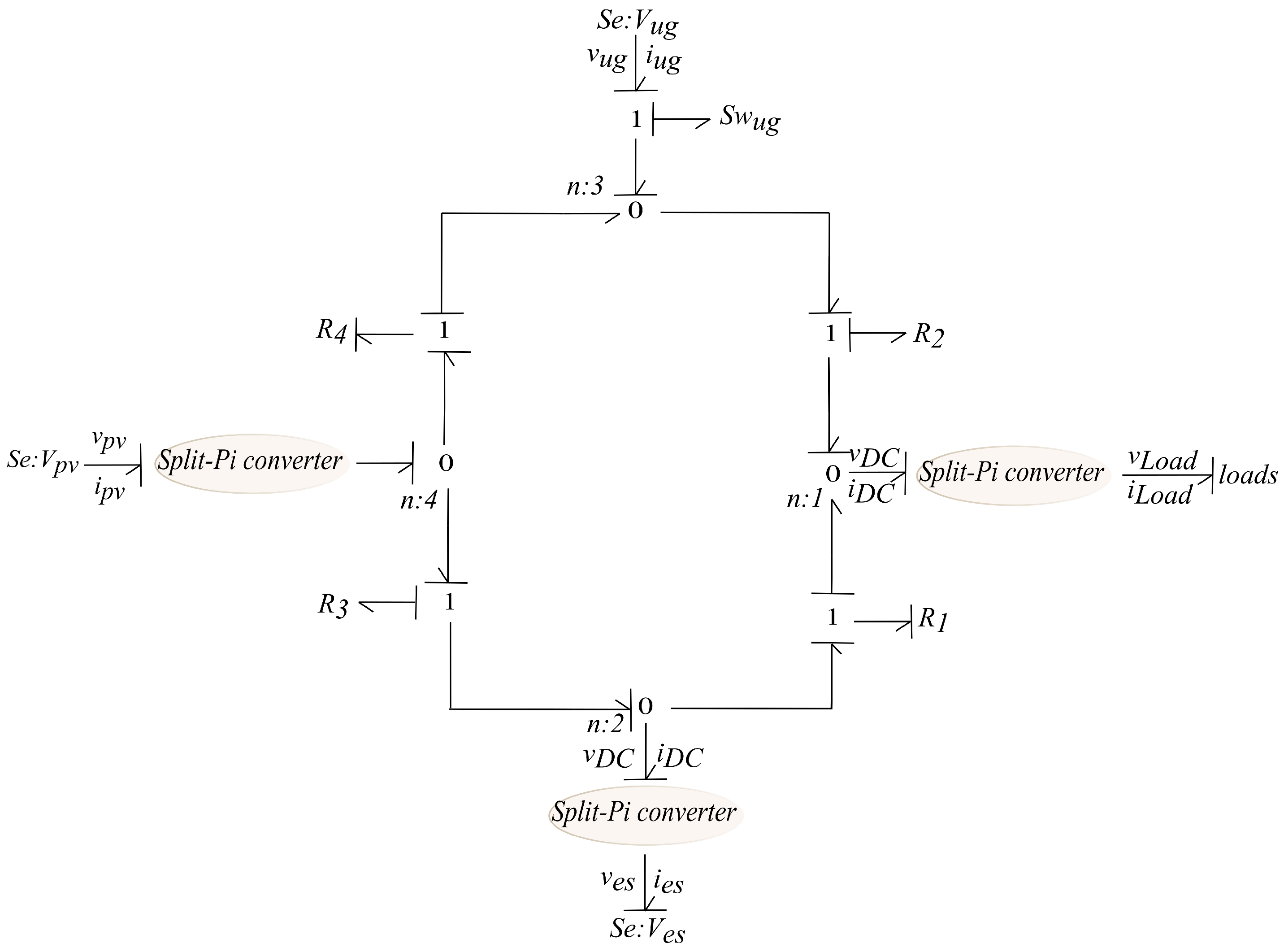
3.2. Dynamical Representation of the DC Bus

The dynamical model of the four-line transmission network (Figure 1) is developed by its Bond graph as already explained in [17]. Ref. [17] provides the Bond graph of the central transmission network taking into account each transmission lines as an RL circuit. In this work, the central network is further simplified eliminating the inductors. In DC networks, the existence of the inductors is necessary only when the current flow of the system varies. However, once the system comes to its steady state, where the current flow remains stable, the inductors have no effect in the DC networks. Hence, each transmission line will be considered as a resistor and the power conservation equation is as follows (Figure 1):

$$P_{pv}\left(t\right)-P_{es}\left(t\right)+P_{ug}\left(t\right)-P_{loads}\left(t\right)-P_R\left(t\right)=0.$$

(3)

$P_{pv,es,ug,loads}$ is the power of the sources and the loads, while $P_R$ is equal to $P_{R_1}+P_{R_2}+P_{R_3}+P_{R_4}$ the power loss for the transmission lines $R_1$,$R_2$,$R_3$,$R_4$. The correspondingly-modified Bond graph of the central DC bus is depicted in Figure 3.

Hence, from the the Bond graph in Figure 3, where only dissipative elements are included, the following is obtained:

$$\begin{array}{cc}\hfill \left[\begin{array}{c}{i}_{pv}\\ i_{ug}\\ i_{es}\\ i_{loads}\end{array}\right]& =\left[\begin{array}{cccc}{\displaystyle \frac{1}{R_3}}+{\displaystyle \frac{1}{R_4}}& -{\displaystyle \frac{1}{R_4}}& -{\displaystyle \frac{1}{R_3}}& 0\\ {\displaystyle \frac{1}{R_4}}& -{\displaystyle \frac{1}{R_4}}-{\displaystyle \frac{1}{R_2}}& 0& {\displaystyle \frac{1}{R_2}}\\ {\displaystyle \frac{1}{R_3}}& 0& -{\displaystyle \frac{1}{R_3}}-{\displaystyle \frac{1}{R_1}}& {\displaystyle \frac{1}{R_1}}\\ 0& {\displaystyle \frac{1}{R_2}}& {\displaystyle \frac{1}{R_1}}& -{\displaystyle \frac{1}{R_1}}-{\displaystyle \frac{1}{R_2}}\end{array}\right]\left[\begin{array}{c}{v}_{pv}\\ v_{ug}\\ v_{es}\\ v_{loads}\end{array}\right].\hfill \end{array}$$

(4)

Therefore, from the above mentioned equations, the current flows on the connecting nodes are deduced as in [13]: (i) $n:1$→$i_{loads}=i_{R_1}+i_{R_2}=\frac{v_{es}-v_{loads}}{R_1}+\frac{v_{ug}-v_{loads}}{R_2}$; (ii) $n:2$→$i_{es}=i_{R_3}-i_{R_1}=\frac{v_{pv}-v_{es}}{R_3}-\frac{v_{es}-v_{loads}}{R_1}$; (iii) $n:3$→$i_{ug}=i_{R_4}-i_{R_2}=\frac{v_{pv}-v_{ug}}{R_4}-\frac{v_{ug}-v_{loads}}{R_2}$; (iv) $n:4$→$i_{pv}=i_{R_3}-i_{R_4}=\frac{v_{pv}\left(t\right)-v_{es}\left(t\right)}{R_3}-\frac{v_{ug}\left(t\right)-v_{pv}\left(t\right)}{R_4}$. The goal is to express all the powers appearing in the grid in terms of voltages and resistances (i.e., to avoid the explicit appearance of currents). Through the relations of the current flows on the connecting nodes previously presented we make use of the fact that the power in every electrical element is $P=i\times v$. Hence, every power variable of the DC network is expressed in function of the voltages on the connecting nodes (see also Figure 1) as in [13]: (i) $P_{pv}=v_{pv}{i}_{pv}=v_{pv}[i_{R_3}-i_{R_4}]=v_{pv}\left[\frac{v_{pv}-v_{es}}{R_3}-\frac{v_{ug}-v_{pv}}{R_4}\right]$; (ii) $P_{es}=v_{es}{i}_{es}=v_{es}[i_{R_3}-i_{R_1}]=v_{es}\left[\frac{v_{pv}-v_{es}}{R_3}-\frac{v_{es}-v_{loads}}{R_1}\right]$; (iii) $P_{ug}=v_{ug}{i}_{ug}=v_{ug}[i_{R_4}-i_{R_2}]=v_{ug}\left[\frac{v_{ug}-v_{pv}}{R_4}-\frac{v_{loads}-v_{ug}}{R_2}\right]$; (iv) $P_{loads}=v_{loads}{i}_{loads}=v_{loads}[i_{R_1}-i_{R_2}]=v_{loads}\left[\frac{v_{es}-v_{loads}}{R_1}-\frac{v_{loads}-v_{ug}}{R_2}\right]$. For the power dissipation within the central transmission network, $P_{R_1}$, $P_{R_2}$, $P_{R_3}$, $P_{R_4}$, we use the other equivalent power formulation, $P=v^2\times R$, which allows deduction of the following relations:

$$\begin{array}{cc}\hfill P_{R_1}& =\frac{{[v_{es}-v_{loads}]}^2}{R_1},\hfill \end{array}$$

(5)

$$\begin{array}{cc}\hfill P_{R_3}& =\frac{{[v_{pv}-v_{es}]}^2}{R_3},\hfill \end{array}$$

(6)

$$\begin{array}{cc}\hfill P_{R_2}& =\frac{{[v_{loads}-v_{ug}]}^2}{R_2},\hfill \end{array}$$

(7)

$$\begin{array}{cc}\hfill P_{R_4}& =\frac{{[v_{ug}-v_{pv}]}^2}{R_4}.\hfill \end{array}$$

(8)

The aforementioned equations are significant and will be proved useful later in structuring the objective function in order to handle the power loss minimization problem.

4. Optimization Objectives and Constraints

Hereinafter, the objectives and constraints of the energy management optimization problem will be introduced.

4.1. Objectives

The main objective of this work is the optimal power flow while minimizing the power dissipation in the DC bus (Figure 4). This problem aims to optimize the power flows within the microgrid so as to minimize the power losses during transmission with the minimum electricity cost. Therefore, the general cost function which penalizes the energy dissipation will be divided in two parts:

• The cost minimization, according to which the electricity cost of the UG power purchase will be penalized. The goal is to sell power to the UG, generated by the renewable resources, and to exploit the ES system towards the consumers’ benefit. The cost function which penalizes the electricity cost is written below:

  $$J^1\left(d\left(t\right)\right)={\int }_{t_0}^{t_f}e\left(t\right)P_{ug}={\int }_{t_0}^{t_f}e\left(t\right)(P_{loads}+P_{es}-P_{pv}),$$

  (9)

  where reference profiles will be taken into account for the PV and the loads. The $P_{ug}$ is replaced, exploiting the power conservation law ($P_{ug}=P_{loads}+P_{es}-P_{pv}$), without considering the power loss (3);
• The optimal power flow, minimizing the power dissipation in the DC bus. Therefore, the cost function will be the following:

  $$J^2\left(d\left(t\right)\right)=-{\int }_{t_0}^{t_f}{P}_R.$$

  (10)

  where $P_R$ corresponds to the power dissipation inside the central network (5)–(8). Relation (3) is taken into account.

We observe that in both cases the power conservation is taken into account and the control variable is the duty cycle of the switches in the converters, $d\left(t\right)$. The ES system and the central transmission network will be analytically included in the optimization problem, utilizing the PH models previously developed here and in [12].

4.2. Constraints

At this point, the general constraints considered at the energy management problem will be analyzed. The ES system constitutes a major component of the overall scheme. Concerning the batteries, their limited lifetime demand to respect certain constraints. Hence, the constraints for the ES system are (see also Figure 2):

$$\begin{array}{cc}\hfill q_{1b}^{min}& \le q_{1b}\left(t\right)\le q_{1b}^{max},\hfill \\ \hfill q_{2b}^{min}& \le q_{2b}\left(t\right)\le q_{2b}^{max},\hfill \\ \hfill \mathrm{Charging}\mathrm{mode}:\\ \hfill v_{b,charging}^{min}& \le v_{b,charging}\left(t\right)\le v_{b,charging}^{max},\hfill \\ \hfill i_{b,charging}^{min}& \le i_{b,charging}\left(t\right)\le i_{b,charging}^{max},\hfill \\ \hfill \mathrm{Dischaging}\mathrm{mode}:\\ \hfill v_{b,dicharging}^{min}& \le v_{b,dicharging}\left(t\right)\le v_{b,dicharging}^{max},\hfill \\ \hfill i_{b,dicharging}^{min}& \le i_{b,dicharging}\left(t\right)\le i_{b,dicharging}^{max}.\hfill \end{array}$$

Furthermore, the voltage on the connecting nodes should always be close to $v_{DC}$ = 400 V. Therefore, the constraints of the connecting nodes are mentioned as follows ($v_{DC}^{min,h}$ and $v_{DC}^{max,h}$ will be the limits of the DC voltage on every connecting node which will be close to the nominal, $v_{DC}=400$ V) (Figure 1):

$$\begin{array}{c}\hfill \begin{array}{cc}\hfill v_{DC}^{min,h}\le & v_{ug}\left(t\right)\le v_{DC}^{max,h},\hfill \end{array}\end{array}$$

(11a)

$$\begin{array}{c}\hfill \begin{array}{cc}\hfill v_{DC}^{min,h}\le & v_{pv}\left(t\right)\le v_{DC}^{max,h},\hfill \end{array}\end{array}$$

(11b)

$$\begin{array}{c}\hfill \begin{array}{cc}\hfill v_{DC}^{min,h}\le & v_{es}\left(t\right)\le v_{DC}^{max,h},\hfill \end{array}\end{array}$$

(11c)

$$\begin{array}{c}\hfill \begin{array}{cc}\hfill v_{DC}^{min,h}\le & v_{loads}\left(t\right)\le v_{DC}^{max,h}.\hfill \end{array}\end{array}$$

(11d)

Additionally, constraints for the duty cycles $d_{1sc}$ and $d_{2sc}$ of the Split-Pi converter are considered as shown below:

$$\begin{array}{cc}\hfill 0& \le d_{1sc}\le 1,\hfill \end{array}$$

(12)

$$\begin{array}{cc}\hfill 0& \le d_{2sc}\le 1.\hfill \end{array}$$

(13)

Finally, maximum and minimum limits for the external grid power generation must be considered:

$$P_{ug}^{min}\le P_{ug}\left(t\right)\le P_{ug}^{max},$$

(14)

with $P_{ug}\left(t\right)=v_{ug}\left(t\right)i_{ug}\left(t\right)$.

ES System Flat Representation

In this subsection, for the ES flat representation (1a)–(1g), the flat outputs are already described in our previous work in [12] and are recalled here for a clear understanding of the proposed approach: (i) $z_1\left(t\right)={\displaystyle \frac{1}{I_{1sc}}}{\displaystyle \frac{p_{1sc}{\left(t\right)}^2}{2}}+{\displaystyle \frac{1}{I_{2sc}}}{\displaystyle \frac{p_{2sc}{\left(t\right)}^2}{2}}+{\displaystyle \frac{1}{C_{2sc}}}{\displaystyle \frac{q_{2sc}{\left(t\right)}^2}{2}}$; (ii) $z_2\left(t\right)=q_{3sc}\left(t\right)+q_{1b}\left(t\right)$; (iii) $z_3\left(t\right)=q_{2b}\left(t\right)$; (iv) $z_4\left(t\right)=q_{2sc}\left(t\right)$. Replacing the aforementioned flat outputs into the PH model (1a)–(1g), the flat representation of the system is acquired, as well as the flat representation of the states and the inputs of the system.

Since the ES system has been already written in terms of the flat outputs, the ES voltage and the current, $v_{es}\left(t\right)$ and $i_{es}\left(t\right)$, can be written in function of a family of N B-splines functions of order d which are denoted as $b_{i,d}\left(t\right)$. These basis functions are summed together (and weighted through their control points $p_i$) in order to describe the flat output $z_3\left(t\right)$. Hence, writing the flat output $z_3$ in function of the B-spline curves, $z_3\left(t\right)={\sum }_{i=1}^N{\mathit{p}}_i{\mathit{b}}_{i,\mathit{d}}\left(t\right)=\mathcal{P}{\mathcal{B}}_d\left(t\right)$, we can now express (15a) and (15b) by exploiting the derivation property of B-splines (which allows characterization of derived splines in terms of lower order splines; matrices $M_{d,d-1}$, $S_{k,d-1,d}$ are computed accordingly as may be seen for example in [22]). Through the B-spline derivation property, we parametrize firstly the voltage of the battery, $v_b$, and the current of the battery, $i_b$, in function of which the ES voltage and the current, $v_{es}\left(t\right)$ and $i_{es}\left(t\right)$, are written: (i) $v_{es}\left(t\right)={\displaystyle \frac{v_b\left(t\right)+i_b\left(t\right)R_{1b}}{\alpha \left(t\right)}}+R_{1sc}\alpha \left(t\right)i_b\left(t\right)$; (ii) $i_{es}\left(t\right)=\alpha \left(t\right)i_b\left(t\right)$ [13]. Therefore, we have the following:

$$\begin{array}{c}\hfill \begin{array}{cc}\hfill {\mathit{p}}_i^{v_b}& ={\displaystyle \frac{1}{C_{2b}}}{p}_i+R_{2b}{\left(\mathcal{P}{M}_{\mathit{d},\mathit{d}-1}{S}_{\kappa ,\mathit{d}-1,\mathit{d}}\right)}_i,\hfill \end{array}\end{array}$$

(15a)

$$\begin{array}{c}\hfill \begin{array}{cc}\hfill {\mathit{p}}_i^{i_b}& =\left(1+{\displaystyle \frac{C_{1b}}{C_{2b}}}\right){\left(\mathcal{P}{M}_{\mathit{d},\mathit{d}-1}{S}_{\kappa ,\mathit{d}-1,\mathit{d}}\right)}_i+C_{1b}{R}_{2b}·{\left(\mathcal{P}{M}_{\mathit{d},\mathit{d}-2}{S}_{\kappa ,\mathit{d}-2,\mathit{d}}\right)}_i,\hfill \end{array}\end{array}$$

(15b)

where $p_i^{i_b}$ and $p_i^{v_b}$ are the control points for the battery’s current and voltage, respectively. Next, for $v_b\left(t\right)$ and $i_b\left(t\right)$ as already presented in [12], we have:

$$\begin{array}{c}\hfill \begin{array}{cc}\hfill v_b\left(t\right)& ={\mathit{b}}_{i,\mathit{d}}\left(t\right)\sum _{i=1}^N\left[{\displaystyle \frac{1}{C_{2b}}}{p}_i+R_{2b}{\left(\mathcal{P}{M}_{\mathit{d},\mathit{d}-1}{S}_{\kappa ,\mathit{d}-1,\mathit{d}}\right)}_i\right],\hfill \end{array}\end{array}$$

(16a)

$$\begin{array}{c}\hfill \begin{array}{cc}\hfill i_b\left(t\right)& ={\mathit{b}}_{i,\mathit{d}}\left(t\right)\sum _{i=1}^N\left[\left(1+{\displaystyle \frac{C_{1b}}{C_{2b}}}\right){\left(\mathcal{P}{M}_{\mathit{d},\mathit{d}-1}{S}_{\kappa ,\mathit{d}-1,\mathit{d}}\right)}_i+C_{1b}{R}_{2b}{\left(\mathcal{P}{\mathcal{M}}_{\mathit{d},\mathit{d}-2}{\mathcal{S}}_{\kappa ,\mathit{d}-2,\mathit{d}}\right)}_i\right],\hfill \\ & \phantom{a}\forall t\in \left[{\tau }_{\kappa }{\tau }_{\kappa +1}\right).\hfill \end{array}\end{array}$$

(16b)

All the variables and the parameters of the Equations (16a) and (16b) are introduced and explained in the notations section.

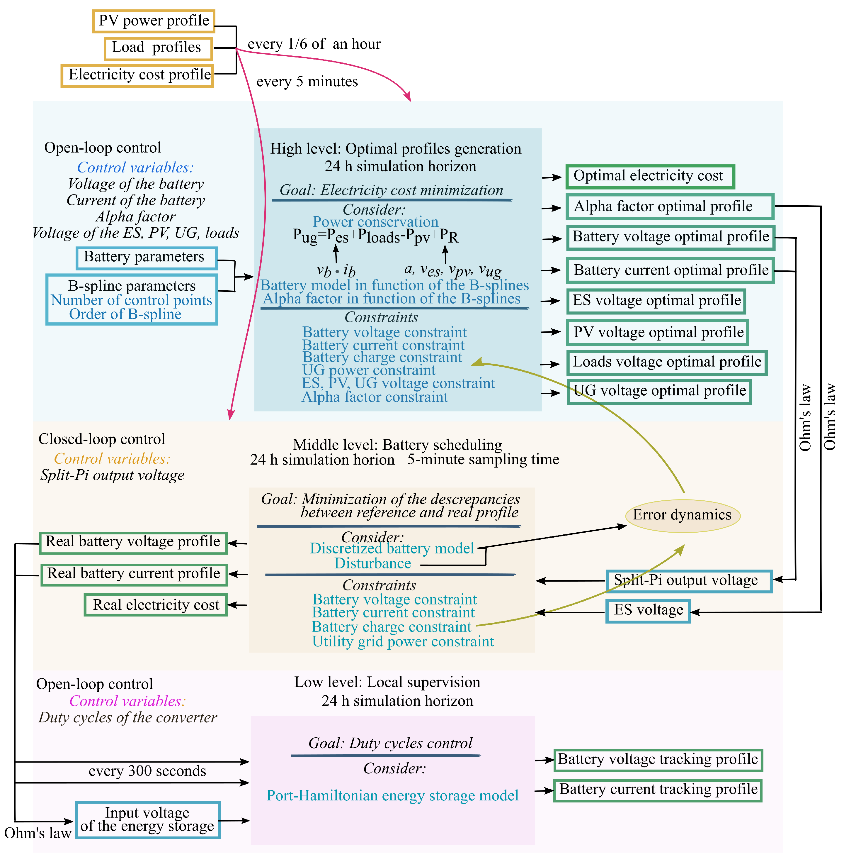
5. Hierarchical Control Approach with Constrained Optimization

This section presents the hierarchical control problem analytically, describing the high and the middle level including the power dissipation. The high level profiles for the ES, $P_{es}$, and the UG, $P_{ug}$, are generated by mitigating the electricity cost and the power losses. At the high and the middle level, the whole dynamics of the ES system is taken into account, as will be shown later, in order to link the power losses of the central transmission network to the battery dynamics. Afterwards, the acquired high level profiles are used as references at the middle level for tracking under perturbation. The discretized model of the battery is considered, already presented in [12], and the main objective is to minimize the deviations amongst the reference and the real values. Finally, at the low level, the tracking profiles of the voltage and the current of the battery, as well as the input voltage of the ES system, $v_{es}$, are applied to the ES PH model to control the switches.

As aforementioned, the flatness-based optimization approach of [12] is reformulated adding the power losses within the central network as in Figure 1. Therefore, the dynamics of the system change and the problem becomes more complicated because of the relations among the voltage, the current and the power of the DERs, the consumers’ demand and the power losses. In the present case, since the power losses in the central transmission lines are considered, the voltage in the common DC-bus will not be stable and it will vary regarding the constraints of (11a)–(11d). On each connecting node a different voltage value will appear, because of the voltage drop created by the resistors. Therefore, a different notation for the voltage and the current on each connecting node is necessary.

In Figure 5, the control scheme of the energy management problem, under the presence of the power dissipation, is illustrated. Optimal profiles are generated for the ES system, the duty cycles through the $\alpha$ factor and the voltages on the connecting nodes.

5.1. High Level

This section will introduce the optimization problem of the high level including details for its flat representation and B-spline parametrization for continuous-time constraint validation.

Definition of the Optimization Problem with the Power Loss Included

The principal objective of the high level problem is the generation of reference trajectories in continuous time, exploiting the flat output representation of the ES system. Therefore, an optimal scheduling for the battery charging and discharging is obtained and, in the meantime, the electrical power purchase from the UG is minimized. The general cost function considered at the high level is the following:

$$\mathcal{J}={\int }_{t_0}^{t_f}e\left(t\right)P_{ug}dt,$$

(17)

where $e\left(t\right)$ is the electricity price.

At first, the power losses are taken into consideration (3), hence $P_{ug}\left(t\right)$ is equal to:

$$\begin{array}{cc}\hfill P_{ug}\left(t\right)=& P_{loads}\left(t\right)+P_R\left(t\right)+P_{es}\left(t\right)-P_{pv}\left(t\right)\hfill \\ \hfill P_{es}\left(t\right)=& -P_{loads}\left(t\right)-P_R\left(t\right)+P_{pv}\left(t\right)+P_{ug}\left(t\right),\hfill \end{array}$$

(18)

Hereinafter, the objective function is analytically calculated and has the following form:

$$\mathcal{J}={\int }_{t_0}^{t_f}e\left(t\right)\left(P_{loads}\left(t\right)+P_R\left(t\right)+P_{es}\left(t\right)-P_{pv}\left(t\right)\right)dt$$

(19)

and the complete optimization problem becomes:

$$\begin{array}{c}\hfill \begin{array}{cc}\hfill \underset{\alpha ,v_{ug},v_{pv},v_{es},v_b,i_b}{min}{\int }_{t_0}^{t_f}e\left(t\right)[P_{loads}& \left(t\right)+P_R\left(t\right)-P_{pv}\left(t\right)+\underset{i_b\left(t\right)v_b\left(t\right)}{\underbrace{P_{es}\left(t\right)}}\left(t\right)]dt,\hfill \end{array}\end{array}$$

(20a)

$$\begin{array}{c}\hfill \begin{array}{cc}\hfill subject\phantom{a}to:\phantom{.}the\phantom{.}syste& m\phantom{.}dynamics\phantom{.}\left(1a\right)-\left(1g\right),\hfill \end{array}\end{array}$$

(20b)

$$\begin{array}{c}\hfill \begin{array}{cc}\hfill \phantom{.}the\phantom{.}power& \phantom{.}conservation\phantom{.}\left(18\right),\hfill \end{array}\end{array}$$

(20c)

$$\begin{array}{c}\hfill \begin{array}{cc}\hfill v_{DC}^{min,h}\le v_{loads}\left(t\right),v_{es}\left(t\right),v_{pv}& \left(t\right)v_{ug}\left(t\right)\le v_{DC}^{max,h},\hfill \end{array}\end{array}$$

(20d)

$$\begin{array}{c}\hfill \begin{array}{cc}\hfill v_b^{min,h}\le & v_b\left(t\right)\le v_b^{max,h},\hfill \end{array}\end{array}$$

(20e)

$$\begin{array}{c}\hfill \begin{array}{cc}\hfill i_b^{min,h}\le & i_b\left(t\right)\le i_b^{max,h},\hfill \end{array}\end{array}$$

(20f)

$$\begin{array}{c}\hfill \begin{array}{cc}\hfill q_{2b}^{min,h}\le & q_{2b}\left(t\right)\le q_{2b}^{max,h},\hfill \end{array}\end{array}$$

(20g)

$$\begin{array}{c}\hfill \begin{array}{cc}\hfill P_{ug}^{min,h}+P_{pv}\left(t\right)& -P_{loads}\left(t\right)-P_R\left(t\right)\le P_{es}\left(t\right)\hfill \\ \hfill P_{es}\left(t\right)\le P_{ug}^{max,h}-& P_{pv}\left(t\right)+P_{loads}\left(t\right)-P_R\left(t\right).\hfill \end{array}\end{array}$$

(20h)

Additionally, the following are also considered to write the final form of the objective function of (20a):

• the voltage, $v_{loads}$, on the connecting node 1 is written in function of the input voltage, $v_{es}$, and the input current, $i_{es}$, of the ES system:

  $$v_{loads}\left(t\right)=R_1{i}_{es}\left(t\right)+(1+{\displaystyle \frac{R_1}{R_3}})v_{es}\left(t\right)-{\displaystyle \frac{R_1}{R_3}}{v}_{pv}\left(t\right);$$

  (21)
• the constraint for the consumer’s demand is considered as follows:

  $$\begin{array}{cc}\hfill P_{loads}\left(t\right)-{ϵ}_{loads}\le & \left[{\displaystyle \frac{-v_{loads}\left(t\right)+v_{es}\left(t\right)}{R_1}}-{\displaystyle \frac{-v_{ug}\left(t\right)+v_{loads}\left(t\right)}{R_2}}\right]v_{loads}\left(t\right)\le \hfill \\ \hfill \le & P_{loads}\left(t\right)+{ϵ}_{loads},\hfill \end{array}$$

  (22)

  where ${ϵ}_{loads}$ is the soft constraint to relax the consumers’ demand in order to guarantee that the optimization problem will be resolvable.

The voltages on the connecting nodes, $v_{es}$, $v_{ug}$, $v_{loads}$ and $v_{pv}$, obey to (11a)–(11d). Finally, the $\alpha \left(t\right)$ factor and the $P_{ug}\left(t\right)$ (taking into account also (18)) will be:

$$\begin{array}{c}\hfill \begin{array}{cc}\hfill 0<\alpha \left(t\right)<1& ,\hfill \end{array}\end{array}$$

(23a)

$$\begin{array}{c}\hfill \begin{array}{cc}\hfill P_{ug}^{min,h}\le P_{ug}\left(t\right)\le & P_{ug}^{max,h}\hfill \end{array}\end{array}$$

(23b)

$$\begin{array}{c}\hfill \begin{array}{cc}\hfill P_{ug}^{min,h}\le P_{loads}\left(t\right)+P_{es}\left(t\right)-P_{pv}& \left(t\right)+P_R\left(t\right)\le P_{ug}^{max,h}.\hfill \end{array}\end{array}$$

(23c)

5.2. Flat Representation and B-Spline Parametrization of the Optimization Problem

Next, the optimization problem in (20a)–(20h) is revised in terms of the flat outputs. The cost function is expressed in terms of the relations in (5)–(8). The flat representations of the $v_{es}\left(t\right)$ and $i_{es}\left(t\right)$ variables of the ES system are deduced in terms of the flat representations of the battery’s current and voltage, $i_b\left(t\right)$ and $v_b\left(t\right)$, as previously presented in [12]. Substituting (5)–(8) in (19), the cost function becomes:

$$\begin{array}{c}\hfill \begin{array}{cc}\hfill \mathcal{J}=\underset{t_0}{\overset{t_f}{\int }}e\left(t\right)& [Q_{cost}\left(P_{loads}\left(t\right)+\underset{v_{es}\left(t\right)i_{es}\left(t\right)}{\underbrace{P_{es}\left(t\right)}}-P_{pv}\left(t\right)\right)+Q_{loss}({\displaystyle \frac{-v_{loads}\left(t\right)+{\left(v_{es}\left(t\right)\right)}^2}{R_1}}+\hfill \\ \hfill +& {\displaystyle \frac{-v_{ug}\left(t\right)+{\left(v_{loads}\left(t\right)\right)}^2}{R_2}}+{\displaystyle \frac{-v_{pv}\left(t\right)+{\left(v_{ug}\left(t\right)\right)}^2}{R_4}}+{\displaystyle \frac{-v_{es}\left(t\right)+{\left(v_{pv}\left(t\right)\right)}^2}{R_3}}\left)\right]\mathrm{d}t.\hfill \end{array}\end{array}$$

(24)

Since $i_{es}\left(t\right)$ and $v_{es}\left(t\right)$ are in function of the battery’s current and voltage, $i_b$ and $v_b$, they can be parametrized in terms of the B-splines according to (16a) and (16b). Similarly, (23a) and (23b) must be also parametrized in terms of the B-splines. The $\alpha$ factor is, firstly, parametrized considering ${\displaystyle \frac{1}{\alpha \left(t\right)}}\in (1,+\infty )$ and a group of B-splines basis functions with $d_{\alpha }$ order as it is written below:

$$\begin{array}{c}\hfill \alpha {\left(t\right)}^{-1}=\sum _{j=1}^{N_{\alpha }}{p}_j^{\alpha }{\mathit{b}}_{i,{\mathit{d}}_{\alpha }}\left(t\right).\end{array}$$

(25)

The number of control points ${\mathit{p}}_i^{\alpha }$ is deduced as $N_{\alpha }$. Then, applying Theorem A1 from Appendix A, a sufficient condition for ensuring (20a) is that each of the scalar control points are supraunitary:

$${\mathit{p}}_i^{\alpha }>1,\forall i=1,\cdots ,N_{\alpha }.$$

(26)

Since $\alpha$ lies in the interval of $(0,1)$, meaning that it is positive, the following can be considered for the second part of $v_{es}$:

$$-R_{1sc}|i_b\left(t\right)|\le R_{1sc}\alpha \left(t\right)i_b\left(t\right)\le R_{1sc}\left|i_b\left(t\right)\right|.$$

(27)

Therefore, the constraint $v_{DC}^{min,h}\le v_{es}\left(t\right)\le v_{DC}^{max,h}$, where $v_{es}$ is considered, is valid if and only if:

$$\begin{array}{c}\hfill \begin{array}{c}\hfill {\displaystyle \frac{v_b\left(t\right)+i_b\left(t\right)R_{1b}}{\alpha \left(t\right)}}-R_{1sc}\left|i_b\left(t\right)\right|\ge v_{DC}^{min,h},\end{array}\end{array}$$

(28a)

$$\begin{array}{c}\hfill \begin{array}{c}\hfill {\displaystyle \frac{v_b\left(t\right)+i_b\left(t\right)R_{1b}}{\alpha \left(t\right)}}+R_{1sc}\left|i_b\left(t\right)\right|\le v_{DC}^{max,h}.\end{array}\end{array}$$

(28b)

Then, for (11a)–(11d) and (23b)), $v_{es}$, $i_{es}$ and $P_{es}$ are combined to arrive at the following:

$$\begin{array}{c}\hfill \begin{array}{c}\hfill \left({\mathit{p}}_i^{v_b}+R_{1b}{\mathit{p}}_i^{i_b}\right){\mathit{p}}_j^{\alpha }-R_{1sc}\left|{\mathit{p}}_i^{i_b}\right|\ge v_{DC}^{min,h},\end{array}\end{array}$$

(29a)

$$\begin{array}{c}\hfill \begin{array}{c}\hfill \left({\mathit{p}}_i^{v_b}+R_{1b}{p}_i^{i_b}\right){\mathit{p}}_j^{\alpha }+R_{1sc}\left|{\mathit{p}}_i^{i_b}\right|\le v_{DC}^{max,h},\end{array}\end{array}$$

(29b)

where ${\mathit{p}}_{\kappa ,i}^{v_b}$ and ${\mathit{p}}_{\kappa ,i}^{i_b}$ are defined by (15a) and (15b) and $\kappa$, i and $j\in \mathbb{N}$ satisfy $\mathit{d}-1\le \kappa \le n-1$, $\kappa -\mathit{d}+2\le i\le \kappa +1$ and $1\le j\le N_{\alpha }$. After various computations, which is given explicitly in Appendix B, the previous inequalities are replaced by the sufficient formulations:

$$\begin{array}{c}\hfill \begin{array}{cc}\hfill v_{DC}^{min,h}& \le \sum _{i=1}^N\sum _{j=1}^{N_{\alpha }}({\mathit{p}}_i^{v_b}+R_{1b}{\mathit{p}}_i^{i_b}){\mathit{p}}_j^{\alpha }{\mathit{b}}_{i,j,\mathit{d}}\left(t\right)-\sum _{i=1}^N\sum _{j=1}^{N_{\alpha }}{R}_{1sc}\left|{\mathit{p}}_i^{i_b}\right|{\mathit{p}}_j^{\alpha }{\mathit{b}}_{i,j,\mathit{d}}\left(t\right)\le \hfill \\ \hfill & \le \sum _{i=1}^N\sum _{j=1}^{N_{\alpha }}\left[{\mathit{p}}_i^{v_b}+R_{1b}{\mathit{p}}_i^{i_b}-R_{1sc}\left|{\mathit{p}}_i^{i_b}\right|\right]{\mathit{p}}_j^{\alpha }{\mathit{b}}_{i,j,\mathit{d}}\left(t\right),\hfill \end{array}\end{array}$$

(30a)

$$\begin{array}{c}\hfill \begin{array}{cc}\hfill v_{DC}^{max,h}& \ge \sum _{i=1}^N\sum _{j=1}^{N_{\alpha }}({\mathit{p}}_i^{v_b}+R_{1b}{\mathit{p}}_i^{i_b}){\mathit{p}}_j^{\alpha }{\mathit{b}}_{i,j,\mathit{d}}\left(t\right)+\sum _{i=1}^N\sum _{j=1}^{N_{\alpha }}{R}_{1sc}\left|{\mathit{p}}_i^{i_b}\right|{\mathit{p}}_j^{\alpha }{\mathit{b}}_{i,j,\mathit{d}}\left(t\right)\ge \hfill \\ \hfill & \ge \sum _{i=1}^N\sum _{j=1}^{N_{\alpha }}\left[({\mathit{p}}_i^{v_b}+R_{1b}{\mathit{p}}_i^{i_b})+R_{1sc}\left|{\mathit{p}}_i^{i_b}\right|\right]{\mathit{p}}_j^{\alpha }{\mathit{b}}_{i,j,\mathit{d}}\left(t\right).\hfill \end{array}\end{array}$$

(30b)

Concerning the $P_{ug}$ constraint and taking into account the $i_{ug}$ current flow on the connecting node $n:1$ as previously mentioned, it is defined below:

$$\begin{array}{cc}\hfill P_{ug}\left(t\right)=& i_{ug}\left(t\right)v_{ug}\left(t\right)=v_{ug}\left(t\right)[i_{R_4}\left(t\right)-i_{R_2}\left(t\right)]=v_{ug}\left(t\right)({\displaystyle \frac{-v_{pv}\left(t\right)+v_{ug}\left(t\right)}{R_4}}-\hfill \\ \hfill -& {\displaystyle \frac{-v_{ug}\left(t\right)+v_{loads}\left(t\right)}{R_2}})=v_{ug}^2\left(t\right)\left({\displaystyle \frac{1}{R_2}}+{\displaystyle \frac{1}{R_4}}\right)-\left({\displaystyle \frac{v_{loads}\left(t\right)}{R_2}}+{\displaystyle \frac{v_{pv}\left(t\right)}{R_4}}\right)v_{ug}\left(t\right).\hfill \end{array}$$

(31)

Replacing $v_{loads}\left(t\right)$ with (21) leads to:

$$\begin{array}{cc}\hfill P_{ug}\left(t\right)=v_{ug}^2\left(t\right)\left({\displaystyle \frac{1}{R_4}}+{\displaystyle \frac{1}{R_2}}\right)-{\displaystyle \frac{1}{R_4}}{v}_{ug}& \left(t\right)v_{pv}\left(t\right)-v_{ug}\left(t\right)[R_1{i}_{es}\left(t\right)+\hfill \\ \hfill & +\left(1+{\displaystyle \frac{R_1}{R_3}}\right)v_{es}\left(t\right)-{\displaystyle \frac{R_1}{R_3}}{v}_{pv}\left(t\right)].\hfill \end{array}$$

(32)

Including also the relations amongst $v_{es}$ and $i_{es}$ with $v_b$ and $i_b$, as presented also in [13], $P_{ug}\left(t\right)$ is denoted as:

$$\begin{array}{cc}\hfill P_{ug}\left(t\right)& =\left({\displaystyle \frac{1}{R_2}}+{\displaystyle \frac{1}{R_4}}\right)v_{ug}^2\left(t\right)+\left({\displaystyle \frac{R_1}{R_3{R}_2}}-{\displaystyle \frac{1}{R_4}}\right)v_{pv}\left(t\right)v_{ug}\left(t\right)-\hfill \\ \hfill & -v_{ug}\left(t\right){\displaystyle \frac{1}{R_2}}\left[\alpha \left(t\right)i_b\left(t\right)R_1+\left(1+{\displaystyle \frac{R_1}{R_3}}\right){\displaystyle \frac{v_b\left(t\right)+R_{1b}{i}_b\left(t\right)}{\alpha \left(t\right)}}+\alpha \left(t\right)i_b\left(t\right)R_{1sc}\right]=\hfill \\ \hfill & =v_{ug}^2\left(t\right)\left({\displaystyle \frac{1}{R_2}}+{\displaystyle \frac{1}{R_4}}\right)+v_{pv}\left(t\right)v_{ug}\left(t\right)\left({\displaystyle \frac{R_1}{R_2{R}_3}}-{\displaystyle \frac{1}{R_4}}\right)-\hfill \\ \hfill & -v_{ug}\left(t\right){\displaystyle \frac{1}{R_2}}\left[\left({\displaystyle \frac{R_1}{R_3}}+1\right){\displaystyle \frac{v_b\left(t\right)+i_b\left(t\right)R_{1b}}{\alpha \left(t\right)}}+\left({\displaystyle \frac{R_1{R}_{1sc}}{R_3}}+R_1+R_{1sc}\right)\alpha \left(t\right)i_b\left(t\right)\right].\hfill \end{array}$$

(33)

Therefore, finally, the constraint (23b) is defined as:

$$\begin{array}{c}\hfill \begin{array}{cc}\hfill P_{ug}^{max,h}& \ge ({\displaystyle \frac{1}{R_2}}+{\displaystyle \frac{1}{R_4}})v_{ug}^2\left(t\right)+v_{pv}\left(t\right)v_{ug}\left(t\right)(-{\displaystyle \frac{1}{R_4}}+{\displaystyle \frac{R_1}{R_3{R}_2}})\hfill \\ \hfill & -v_{ug}\left(t\right){\displaystyle \frac{1}{R_2}}\left[(1+{\displaystyle \frac{R_1}{R_3}}){\displaystyle \frac{v_b\left(t\right)+i_b\left(t\right)R_{1b}}{\alpha \left(t\right)}}-\left|i_b\left(t\right)\right|(R_1+R_{1sc}+{\displaystyle \frac{R_{1sc}{R}_1}{R_3}})\right],\hfill \end{array}\end{array}$$

(34a)

$$\begin{array}{c}\hfill \begin{array}{cc}\hfill P_{ug}^{min,h}& \le ({\displaystyle \frac{1}{R_2}}+{\displaystyle \frac{1}{R_4}})v_{ug}^2\left(t\right)+v_{pv}\left(t\right)v_{ug}\left(t\right)({\displaystyle \frac{R_1}{R_3{R}_2}}-{\displaystyle \frac{1}{R_4}})\hfill \\ \hfill & -{\displaystyle \frac{1}{R_2}}{v}_{ug}\left(t\right)\left[(1+{\displaystyle \frac{R_1}{R_3}}){\displaystyle \frac{v_b\left(t\right)+i_b\left(t\right)R_{1b}}{\alpha \left(t\right)}}+\left|i_b\left(t\right)\right|(R_{1sc}{R}_1+R_{1sc}+{\displaystyle \frac{R_1}{R_3}})\right].\hfill \end{array}\end{array}$$

(34b)

Additionally, considering that $-|i_b\left(t\right)|\le \alpha \left(t\right)i_b\left(t\right)\le \left|i_b\left(t\right)\right|$ and ${\displaystyle \frac{v_b\left(t\right)+R_{1b}{i}_b\left(t\right)}{\alpha \left(t\right)}}>0$ we can rewrite the two previous constraints, (34a) and (34b), as follows:

$$\begin{array}{c}\hfill \begin{array}{cc}\hfill (1+{\displaystyle \frac{R_1}{R_3}}){\displaystyle \frac{v_b\left(t\right)+i_b\left(t\right)R_{1b}}{\alpha \left(t\right)}}-& |i_b\left(t\right)|(R_{1sc}+R_1+{\displaystyle \frac{R_{1sc}{R}_1}{R_3}})\ge -{\displaystyle \frac{R_2}{v_{ug}\left(t\right)}}[P_{ug}^{max,h}-\hfill \\ \hfill -v_{ug}^2\left(t\right)({\displaystyle \frac{1}{R_2}}+{\displaystyle \frac{1}{R_4}})& -v_{pv}\left(t\right)v_{ug}\left(t\right)({\displaystyle \frac{R_1}{R_3{R}_2}}-{\displaystyle \frac{1}{R_4}})],\hfill \end{array}\end{array}$$

(35a)

$$\begin{array}{c}\hfill \begin{array}{cc}\hfill (1+{\displaystyle \frac{R_1}{R_3}}){\displaystyle \frac{v_b\left(t\right)+i_b\left(t\right)R_{1b}}{\alpha \left(t\right)}}+& |i_b\left(t\right)|(R_{1sc}+R_1+{\displaystyle \frac{R_{1sc}{R}_1}{R_3}})\le -{\displaystyle \frac{R_2}{v_{ug}\left(t\right)}}[P_{ug}^{min,h}-\hfill \\ \hfill -v_{ug}^2\left(t\right)({\displaystyle \frac{1}{R_2}}+{\displaystyle \frac{1}{R_4}})& -v_{pv}\left(t\right)v_{ug}\left(t\right)({\displaystyle \frac{R_1}{R_3{R}_2}}-{\displaystyle \frac{1}{R_4}})].\hfill \end{array}\end{array}$$

(35b)

Next, through (A1a) and (A1b) in Appendix B, the left part of (35a) and (35b) is defined in terms of the B-splines:

$$\begin{array}{cc}\hfill & ({\displaystyle \frac{R_1}{R_3}}+1){\displaystyle \frac{v_b\left(t\right)+i_b\left(t\right)R_{1b}}{\alpha \left(t\right)}}\pm \left|i_b\left(t\right)\right|(R_{1sc}+R_1+{\displaystyle \frac{R_{1sc}{R}_1}{R_3}})=(1+{\displaystyle \frac{R_1}{R_3}})\hfill \\ \hfill & \sum _{i=1}^N\sum _{j=1}^{N_{\alpha }}({\mathit{p}}_i^{v_b}+R_{1b}{\mathit{p}}_i^{i_b}){\mathit{p}}_j^{\alpha }{\mathit{b}}_{i,j,\mathit{d}}\left(t\right)\pm (R_1+R_{1sc}+{\displaystyle \frac{R_1{R}_{1sc}}{R_3}})\sum _{i=1}^N\sum _{j=1}^{N_{\alpha }}\left|{\mathit{p}}_i^{i_b}\right|{\mathit{b}}_{i,j,\mathit{d}}\left(t\right),\hfill \end{array}$$

(36)

which is proven similarly as in (A2a) and (A2b).

Hence, the optimization problem of (20a)–(20h) becomes:

$$\begin{array}{cc}\hfill & \underset{\mathit{p},{\mathit{p}}^{\alpha },v_{pv}\left(t\right),v_{ug}\left(t\right)}{min}\underset{t_0}{\overset{t_f}{\int }}e\left(t\right)\left[Q_{cost}\right[(v_b\left(t\right)+R_{1b})i_b{\left(t\right)}^2+R_{1sc}{\left(i_b\left(t\right)\right)}^2\alpha \left(t\right)-P_{pv}\left(t\right)+\hfill \end{array}$$

(37a)

$$\begin{array}{c}\hfill +P_{loads}\left(t\right)]+Q_{loss}[{\displaystyle \frac{{({\displaystyle \frac{i_b\left(t\right)R_{1b}+v_b\left(t\right)}{\alpha \left(t\right)}}+-v_{loads}\left(t\right))}^2+R_{1sc}\alpha \left(t\right)i_b\left(t\right)}{R_1}}+\end{array}$$

(37b)

$$\begin{array}{cc}\hfill & +{\displaystyle \frac{{(-v_{ug}\left(t\right)+v_{loads}\left(t\right))}^2}{R_2}}+{\displaystyle \frac{{(v_{pv}\left(t\right)-{\displaystyle \frac{i_b\left(t\right)R_{1b}+v_b\left(t\right)}{\alpha \left(t\right)}}+R_{1sc}{i}_b\left(t\right))}^2\alpha \left(t\right)}{R_3}}+\hfill \end{array}$$

(37c)

$$\begin{array}{cc}\hfill & +{\displaystyle \frac{{(v_{ug}\left(t\right)-v_{pv}\left(t\right))}^2}{R_4}}\left]\right]\mathrm{d}t\hfill \end{array}$$

(37d)

$$\begin{array}{cc}\hfill & subject\phantom{a}to:\phantom{.}the\phantom{.}system\phantom{.}dynamics\phantom{.}\left(1a\right)-\left(1g\right),\hfill \end{array}$$

(37e)

$$\begin{array}{cc}\hfill & \phantom{.}the\phantom{.}power\phantom{.}conservation\phantom{.}\left(18\right),\hfill \end{array}$$

(37f)

$$\begin{array}{cc}\hfill & the\phantom{a}voltage\phantom{a}constraints\phantom{a}on\phantom{a}the\phantom{a}connecting\phantom{a}nodes\phantom{a}\left(11\right)\hfill \end{array}$$

(37g)

$$\begin{array}{cc}\hfill & v_b^{min,h}\le \sum _{i=1}^N{\mathit{b}}_{i,\mathit{d}}\left(t\right){\mathit{p}}_i^{v_b}\le v_b^{max,h},\hfill \end{array}$$

(37h)

$$\begin{array}{cc}\hfill & i_b^{min,h}\le \sum _{i=1}^N{\mathit{b}}_{i,\mathit{d}}\left(t\right){\mathit{p}}_i^{i_b}\le i_b^{max,h},\hfill \end{array}$$

(37i)

$$\begin{array}{cc}\hfill & q_{2b}^{min,h}\le \sum _{i=1}^N{\mathit{b}}_{i,\mathit{d}}\left(t\right){\mathit{p}}_i\le q_{2b}^{max,h},\hfill \end{array}$$

(37j)

$$\begin{array}{cc}\hfill & the\phantom{a}{P}_{ug}\phantom{a}constraints\phantom{a}\left(34a\right),\left(34b\right),\hfill \end{array}$$

(37k)

$$\begin{array}{cc}\hfill & the\phantom{a}central\phantom{a}network\phantom{a}relations\phantom{a}constraints\phantom{a}\left(21\right),\left(22\right).\hfill \end{array}$$

(37l)

$i_b\left(t\right)$ and $v_b\left(t\right)$ are deduced in function of the B-splines as in (16a) and (16b), respectively. $Q_{cost}$ and $Q_{loss}$ are the weight matrices corresponding to the cost minimization and power loss mitigation.

5.3. Middle Level

Next, the middle level of the hierarchical problem will be described. The battery current, $i_b$, battery voltage, $v_b$, and input voltage of the ES system $v_{es}$ reference profiles from the high level will be considered here as $i_b^{ref}$, $v_b^{ref}$ and $v_{es}^{ref}$ correspondingly. Likewise for the $\alpha$ factor which will be referred to as ${\alpha }^{ref}$ at the middle level.

Therefore, we introduce a tube-MPC controller to follow the Split-Pi output voltage reference profile, $v_{sc\_out}^{ref}$, under perturbation. The output voltage reference of the converter is written in function of the battery current and voltage reference profiles from the high level [13]:

$$v_{sc\_out}^{ref}\left(t\right)=v_b^{ref}\left(t\right)+i_b^{ref}\left(t\right)R_{1b},$$

(38)

according to Ohm’s law (Figure 2). We proceed to the battery’s discretization via the standard Euler discretized as already introduced in [12].

At this point, we continue using the tube-MPC controller and the discretized dynamics of the system. However, since the power losses are taken into account, the MPC tracking problem is reformulated as follows:

$$\begin{array}{c}\hfill \begin{array}{cc}\hfill {\displaystyle \underset{\tilde{u}\left(k\right)}{min}\sum _{i=k}^{k+N_p-1}{({\tilde{v}}_{es}\left(i\right)-{\tilde{v}}_{es}^{ref}\left(i\right))}^{\top }{Q}_{{\tilde{v}}_{es}}}& \left({\tilde{v}}_{es}\left(i\right)\right)+\hfill \\ \hfill +{(\tilde{u}\left(i\right)-{\tilde{u}}^{ref}\left(i\right))}^{\top }{R}_{\tilde{u}}& \left(\tilde{u}\left(i\right)-{\tilde{u}}^{ref}\left(i\right)\right)\hfill \end{array}\end{array}$$

(39a)

$$\begin{array}{c}\hfill \begin{array}{cc}\hfill subject\phantom{a}to:\phantom{.}the\phantom{.}system\phantom{.}discr& etized\phantom{.}dynamics,\hfill \end{array}\end{array}$$

(39b)

$$\begin{array}{c}\hfill \begin{array}{cc}\hfill {\tilde{v}}_b^{min,m}\le {\tilde{v}}_b\left(k\right)& \le {\tilde{v}}_b^{max,m},\hfill \end{array}\end{array}$$

(39c)

$$\begin{array}{c}\hfill \begin{array}{cc}\hfill {\tilde{i}}_b^{min,m}\le {\tilde{i}}_b\left(k\right)& \le {\tilde{i}}_b^{max,m},\hfill \end{array}\end{array}$$

(39d)

$$\begin{array}{c}\hfill \begin{array}{cc}\hfill {\tilde{q}}_{2b}^{min,m}\le {\tilde{q}}_{2b}\left(k\right)& \le {\tilde{q}}_{2b}^{max,m},\hfill \end{array}\end{array}$$

(39e)

$$\begin{array}{c}\hfill \begin{array}{cc}\hfill {\tilde{v}}_{es}^{min,m}\le {\tilde{v}}_{es}\left(k\right)& \le {\tilde{v}}_{es}^{max,m},\hfill \end{array}\end{array}$$

(39f)

$$\begin{array}{c}\hfill \begin{array}{cc}\hfill {\tilde{P}}_{ug}^{min,m}\le {\tilde{P}}_{ug}\left(k\right)& \le {\tilde{P}}_{ug}^{max,m}.\hfill \end{array}\end{array}$$

(39g)

In the last constraint, $P_{ug}\left(t\right)$, the power losses must be considered in the power conservation equation as in (18) in Section 5.1. Therefore, (39g) is replaced by:

$$\begin{array}{c}\hfill \begin{array}{c}\hfill {\tilde{P}}_{ug}^{min,m}+{\tilde{P}}_{pv}\left(k\right)-{\tilde{P}}_{loads}\left(k\right)-{\tilde{P}}_R\left(k\right)\le {\tilde{P}}_{es}\left(k\right),\end{array}\end{array}$$

(40a)

$$\begin{array}{c}\hfill \begin{array}{c}\hfill {\tilde{P}}_{ug}^{max,m}+{\tilde{P}}_{pv}\left(k\right)-{\tilde{P}}_{loads}\left(k\right)-{\tilde{P}}_R\left(k\right)\ge {\tilde{P}}_{es}\left(k\right),\end{array}\end{array}$$

(40b)

${\tilde{P}}_{es}\left(k\right)$ is equal to ${\tilde{i}}_{es}\left(k\right){\tilde{v}}_{es}\left(k\right)$ and ${\tilde{P}}_R\left(k\right)$ is equal to ${\tilde{P}}_{R_1}\left(k\right)+{\tilde{P}}_{R_2}\left(k\right)+{\tilde{P}}_{R_3}\left(k\right)+{\tilde{P}}_{R_4}\left(k\right)$. ${\tilde{v}}_{es}\left(k\right)$ and ${\tilde{i}}_{es}\left(k\right)$ are computed regarding the ${\alpha }^{ref}$ obtained at the high level as in [13]:

$$\begin{array}{c}\hfill \begin{array}{cc}\hfill v_{es}\left(k\right)& =\frac{v_b\left(k\right)+i_b\left(k\right)R_{1b}}{{\alpha }^{ref,h}\left(k\right)}+R_{1sc}{\alpha }^{ref}\left(k\right),\hfill \end{array}\end{array}$$

(41a)

$$\begin{array}{c}\hfill \begin{array}{cc}\hfill i_{es}\left(k\right)& ={\alpha }^{ref}\left(k\right)i_b\left(k\right).\hfill \end{array}\end{array}$$

(41b)

At this point, we mention that the low level remains the same as in [12] since it is a local controller concerning the operation of the Split-Pi converter locally and its dynamics are not influenced by the addition of the power dissipation in the DC. The single difference is the input voltage, $v_{es}$, of the ES system on the connecting node 2, which varies among the considered constraints (11a)–(11b). The tracking profiles obtained for the voltage, $v_{es}$, at the middle level are considered.

6. Simulation Results

In this section, the simulation results of the of the high, the middle and the low levels are presented. The DC microgrid parameters, considered for the simulations, are illustrated in

Table 1. Parameters.

Variable	Values	Units
$R_{1sc}$, $R_{1b,2b}$	1, $0.025$, $0.088$	[$\Omega$]
$I_{1sc}$, $I_{2sc}$	$0.25$, $0.25$	[H]
$C_{1sc}$, $C_{2sc}$, $C_{3sc}$	$0.0008$, $0.0008$, $0.0008$	[F]
$C_{1b}$, $C_{2b}$	$86,400$, $21,600$	[F]
$R_1$, $R_2$, $R_3$, $R_4$	1	[$\Omega$]

. The variables and constraints for the high level and the middle level are depicted in

Table 2. High and middle level variables and constraints.

	Variable	Values	Units
	N as in (30a) (30b), (36)	27
High level	$N_a$ as in (30a) (30b), (36)	18
	$d_a$ as in (25)	4
	$v_b^{min,h}\le v_b\le v_b^{max,h}$	12 $\le v_b\le 13$	[V]
	$i_b^{min,h}\le i_b\le i_b^{max,h}$	$-9\le i_b\le 9$	[A]
Constraints	$q_{1b}^{min,m}\le q_{1b}\le q_{1b}^{max,m}$	$288.3\le q_{1b}\le 307.7$	[Ah]
	$q_{2b}^{min,h}\le q_{2b}\le q_{2b}^{max,h}$	$72.5\le q_{2b}\le 77.5$	[Ah]
	$P_{ug}^{min,h}\le P_{ug}\le P_{ug}^{max,h}$	$-2100\le P_{ug}\le 4200$	[W]
	$v_{DC}^{min,h}\le v_{ug,pv,es,loads}\le v_{DC}^{max,h}$	$380\le v_{ug,pv,es,loads}\le 430$	[V]
	$N_p$ as in (39a)	5	[h]
Middle level	$Q_{{\tilde{v}}_{es}}$ as in (39a)	$diag(1,1)$
	$R_{\tilde{u}}$ as in (39a)	800
	$v_b^{min,m}\le {\tilde{v}}_b\le v_b^{max,m}$	$11.9\le {\tilde{v}}_b\le 13.1$	[V]
	$i_b^{min,m}\le {\tilde{i}}_b\le i_b^{max,m}$	$-10.6\le {\tilde{i}}_b\le 10.6$	[A]
Constraints	$q_{1b}^{min,m}\le {\tilde{q}}_{1b}\left(k\right)\le q_{1b}^{max,m}$	$287.6\le {\tilde{q}}_{1b}\left(k\right)\le 308.4$	[Ah]
	$q_{2b}^{min,m}\le {\tilde{q}}_{2b}\le q_{2b}^{max,m}$	$72.3\le {\tilde{q}}_{2b}\le 77.7$	[Ah]
	$P_{ug}^{min,m}\le {\tilde{P}}_{ug}\le P_{ug}^{max,m}$	$-2100\le {\tilde{P}}_{ug}\le 4200$	[W]
	$v_{DC}^{min,h}\le v_{ug,pv,es,loads}\le v_{DC}^{max,h}$	$370\le v_{ug,pv,es,loads}\le 430$	[V]

. Reference profiles for the PV and the loads are considered, obtained considering real irradiation and temperature data. Additionally, for the ES system, we take into account a set of lead acid batteries (AGM 12-165). A DC breaker is used to link the DC microgrid with the UG. We use MATLAB $2015a$ for the simulations and YALMIP optimization toolbox [23] for both high and middle levels in order to be able to use the IPOPT solver [24] which handles nonlinear optimization problems. Concerning the low level, the PH ES system was designed in MATLAB/Simulink with the goal to confirm the appropriate switching activity within the Split-Pi [12].

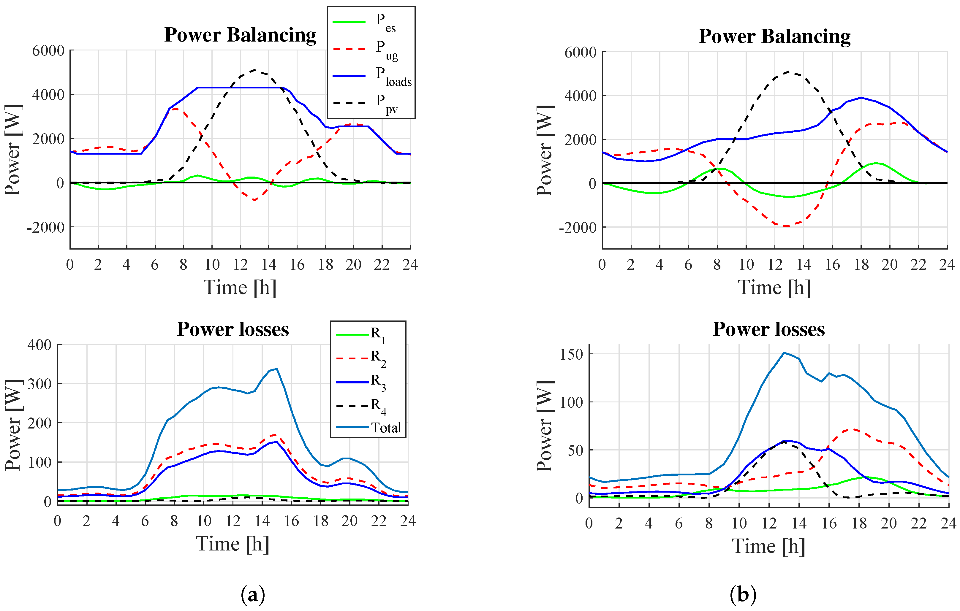
6.1. Simulation Results of the High Level

In this section, the simulation results of the high level are introduced according to (37a)–(37l). The profiles generated at the high level for the commercial use (CU) (Figure 6a), where the load is high during the day, and the domestic use (DU) (Figure 6b), where the load is high during the afternoon, are illustrated. Moreover, the constraints of the system are considered according to the RPI set found in [12].

Concerning the simulations, in the CU case for the $Power$$Balancing$ profiles (Figure 6a) the consuming hours are during the day. The UG cannot completely charge the ES at night, when the cost of the electricity cost is low, because of the power loss existing in the transmission lines (only $0.8\%$ for battery charging). Afterwards, during the day, UG and PV sources collaborate (in total $99\%$ power production) to satisfy the consumers’ demand ($97\%$ consumed from the total power). This is possible considering that we keep same resistor values in the transmission lines, $R=1$$\Omega$. In the case where the batteries are closer to the renewable sources, the losses among them are lower and the batteries could be more effectively charged. Moreover, when the distance among the external grid and the microgrid is higher (meaning higher power loss), then the controller gives priority to the parts which are less affected by the power losses. On the other hand, in DU case the PV and the $UG$ charge the ES from 12 p.m. to 12 a.m. when the demand is low. In the afternoon an increase in the demand is observed, while the rest of the day the demand remains broadly stable. As aforementioned, there is, also, enough energy to sell to the UG, close to $13\%$ of the total consumed power. Hence, to make profit in a commercial environment, the use of larger installations for the renewable resources is important.

Likewise, the batteries’ reference profiles for the voltage, current and state of charge are introduced where the constraints are verified. The electricity cost is also calculated which is $4.318$ euros for the CU and $2.713$ euros for the DU. The cost without using the ES system is $4.737$ euros for the CU profile and $4.732$ euros for the DU profile, where we observe that in the first case (CU profile) remains the same since the ES system usage is almost negligible. Although, in the case of the DU profile, the cost without the battery existence is a lot higher, since its usage is exploited in the best possible way.

Then, Figure 7 depicts the power losses and the constraint validation for the voltage on the connecting nodes. In the CU profile (Figure 7a), the power losses are higher mostly because of the UG power purchase towards the loads during the day (transmission line $R_2$: $0.24\%$ of the total power loss), while in the DU is less (Figure 7b). Furthermore, we observe that the power losses in lines $R_3$ and $R_4$ are similar for both cases because of the PV purchase towards the UG or the ES system. For transmission line $R_1$, with the CU profile, the loss is around $0.12\%$ of the total loss and higher than the DU case since a large amount of power is transmitted from the UG to the loads during the day. While, for the DU, the total loss of $R_1$ and $R_2$, about $0.33\%$, mostly exists due to the fact that the load demand increases during the afternoon. It is visible from

Table 3. Generated and consumed power in relation to the corresponding total power.

Load	Power	Generated Power [%]	Consumed Power [%]	Electricity Cost [Euros]
CU	$P_{ug}$	49.91%	1.78% sold to the UG	4.318
	$P_{es}$	0.79%	0.76% for battery charging	-
	$P_{pv}$	49.30%	-	-
	$P_{loads}$	-	96.9% for the consumers	-
	$P_{loss}$	-	Total: 0.56% $R_{1,2,3,4}$: 0.12%, 0.24%, 0.11%, 0.09%	-
DU	$P_{ug}$	42.14%	13% sold to the UG	2.713
	$P_{es}$	6.58%	6.7% for battery charging	-
	$P_{pv}$	51.28%	-	-
	$P_{loads}$	-	79.66% for the consumers	-
	$P_{loss}$	-	Total: 0.64% $R_{1,2,3,4}$: 0.12%, 0.21%, 0.13%, 0.18%	-

that, finally, the power loss is higher in the CU scenario since also the total power produced is higher than in the case of the DU load profile. The calculation time of the simulation is 12 min for the DU load and 6 min for the CU load.

The previous simulations correspond to the expected results. Since the CU is high during the day, considering also the power losses existing in the transmission line network, the UG is unable to charge the batteries, since it must generate power for the consumers in cooperation with the PV source. In the DU case, since the consumers’ demand is low during the day, similar results are expected as before without including the power losses in the central transmission network. The PV power is able to charge the batteries and sell power to the UG. However, because of the power losses, the power weakens while passing through the transmission lines.

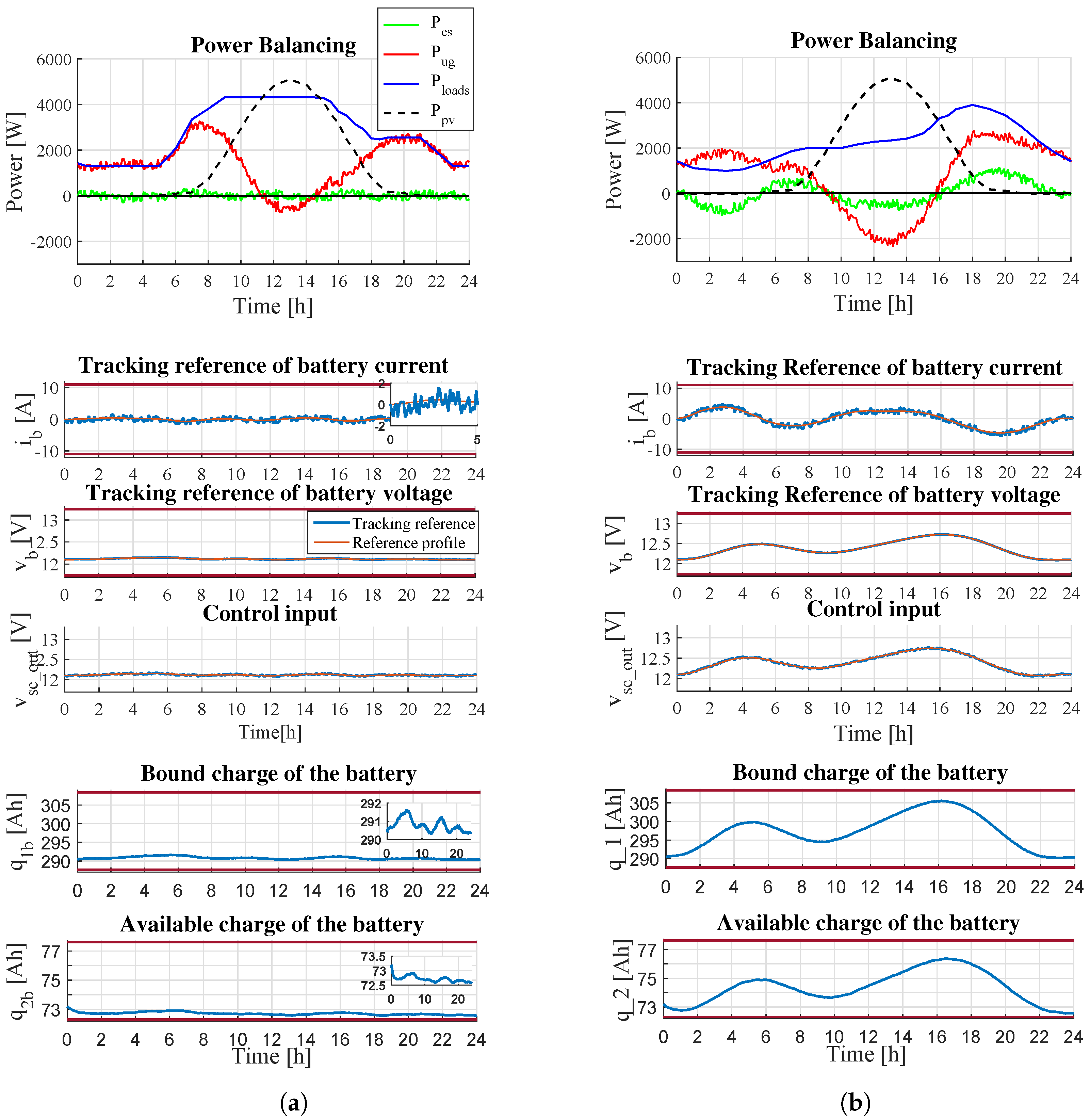
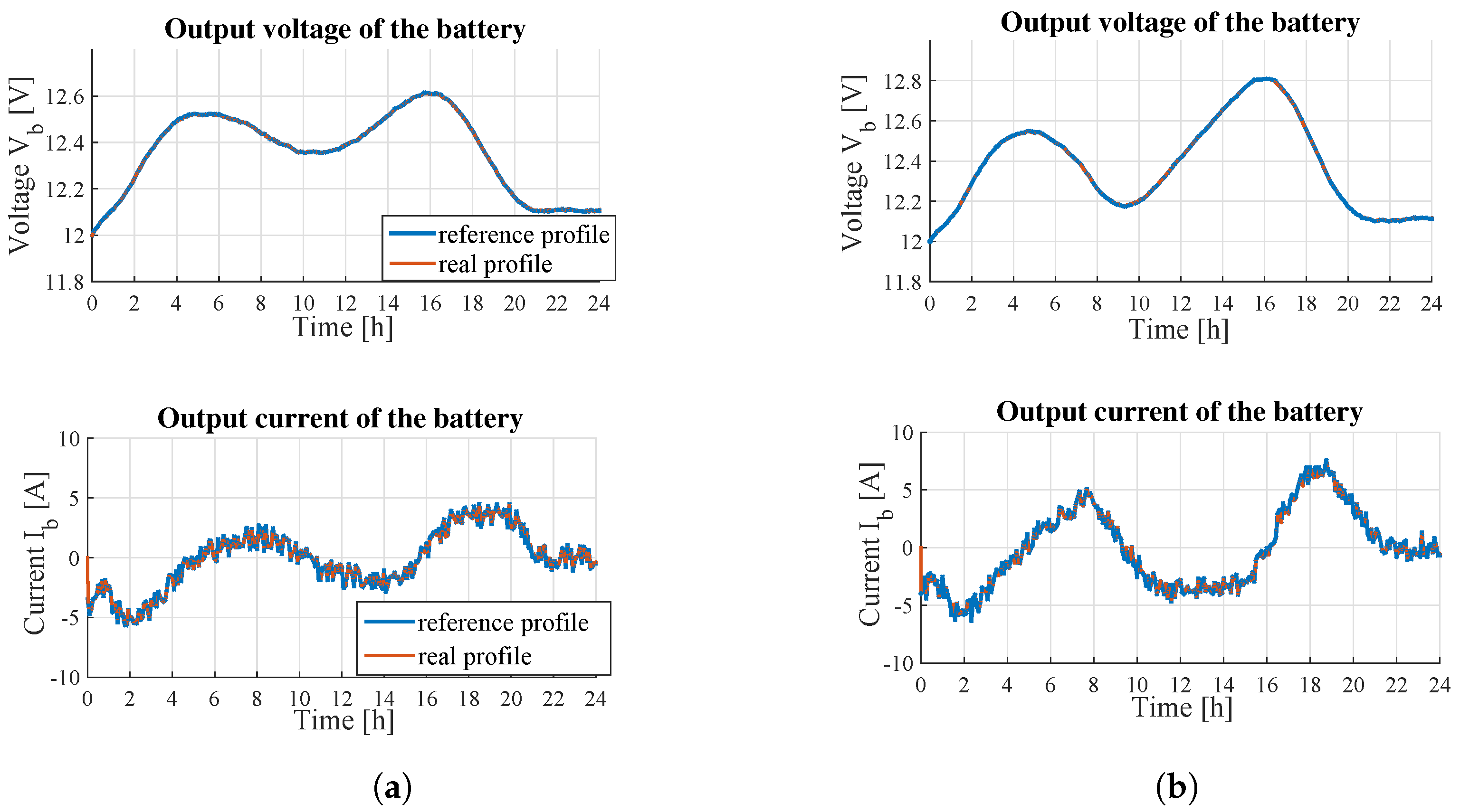
6.2. Simulation Results of the Middle and Low Level

At this section, the middle level results are introduced considering the optimal profiles generated at the high level for the battery current, $i_b$, and the voltage, $v_b$ as references (Figure 6). Table 2 depicts the parameters for the simulations of the middle level. Here, MPC is used for reference tracking considering a prediction horizon $N_p$ equal to 5 and a sampling time $T_s$ equal to 5 min. The system, at this point, is discretized and it follows the optimization problem under constraints as in (39a)–(39g) with losses in the transmission network. Additionally, a perturbation is added to the system that is always lower than the difference between the maximum and minimum state value defined by the RPI set in [12].

Figure 8 shows the middle level profiles of the energy management problem, and the control input, $v_{sc\_out}$ of the Split-Pi converter, in terms of $i_b$ and $v_b$ as in (38). From the figures and the

Table 4. Generated and consumed power in relation to the corresponding total power.

Load Profile	Power	Generated Power [%]	Consumed Power [%]	Generated Power Difference from High Level [%]	Consumed Power Difference from High Level [%]
CU	$P_{ug}$	49.24%	1.85% sold to the UG	−0.62%	0.07%
	$P_{es}$	2.08%	1.84% for battery charging	1.29%	1.05%
	$P_{pv}$	48.68%	-	−0.62%	-
	$P_{loads}$	-	94.74% for the consumers	-	0.75%
	$P_{loss}$	-	1.57%	-	1.01%
DU	$P_{ug}$	41.27%	13.15% sold to the UG	−0.87%	0.08%
	$P_{es}$	7.95%	7.73% for battery charging	1.37%	0.97%
	$P_{pv}$	50.78%	-	−0.5%	-
	$P_{loads}$	-	77.71% for the consumers	-	−1.05%
	$P_{loss}$	-	1.41%	-	0.77%

, where the power produced and the power consumed are illustrated in respect to the total power, we observe that the optimal profiles obtained at the high level are very closely followed.

Furthermore, there are small dissimilarities (less than $1\%$) between the UG power production/consumption reference and the real profiles as well as the battery’s charging/discharging. The cost shortly changes, from $2.713$ to $2.708$ euros for the DU demand and from $4.318$ to $4.308$ euros. The electricity cost decreases slightly, approximately $0.2\%$, since the UG power production decreases and, in parallel, the power sold to the UG increases. Furthermore, the power loss is higher by $1\%$ for the real profiles because of the slight raise of power generated and transmitted from and to the ES system. Although, in general the errors are low and the reference profiles are well followed. The simulations time endure around 14 min for the CU demand and 9 min or the DU demand.

Next, the low level results are presented (Figure 9) tracking the profiles obtained at the middle level for the $i_b$ and the $v_b$ under perturbation (Figure 8). The current, $i_b$, and the voltage, $v_b$, of the battery are considered as the reference profiles to follow, taking into account the control law developed in [12]. Apart from the voltage and current reference profiles of the battery, the reference profile of the voltage, $v_{es}$, entering from the central transmission network is also considered (see Figure 7a,b).

6.3. Optimal Profile Generation of Different Scenarios

Scenario 1: (Different values on the central lines resistors); here, we consider two different scenarios as in

Table 5. Resistor values for Scenario 1.

Load	Resistors	Value	Unit
Commercial	$R_1$	0.5	[$\Omega$]
	$R_2$	5	[$\Omega$]
	$R_3$	5	[$\Omega$]
	$R_4$	0.2	[$\Omega$]
Domestic	$R_1$, $R_4$	1	[$\Omega$]
	$R_2$, $R_3$	3	[$\Omega$]

:

• For the CU profile, the transmission lines $R_1$ and $R_4$ are with different values lower than the $R_2$ and $R_3$ considering a greater distance between the UG and the consumers, the PV and the ES than in the previous case;
• For the DU profile, the transmission lines $R_1$ and $R_4$ are equal to 1 $\Omega$ (as in Section 6.1) and $R_2$ and $R_3$ are equal to 3 $\Omega$ keeping this way the renewable resource closer to the UG and the ES closer to the loads.

In the first case and according to Figure 10 and

Table 6. Simulation results obtained of Scenario 1.

Load	Power	Generated Power [%]	Consumed Power [%]	Electricity Cost (Euros)
CU	$P_{ug}$	51.2%	1.9% sold to the UG	4.623
	$P_{es}$	1.9%	2% for battery charging	-
	$P_{loads}$	-	92% for the consumers	-
	$P_{pv}$	46.9%	-	-
	$P_{loss}$	-	Total: 4.1% $R_{1,2,3,4}$: 0.19%, 2.1%, 1.76%, 0.05%	-
DU	$P_{ug}$	44%	13.1% sold to the UG	2.857
	$P_{es}$	6%	6.7% for battery charging	-
	$P_{loads}$	-	78.1% for the consumers	-
	$P_{pv}$	50%	-	-
	$P_{loss}$	-	Total: 2.1% $R_{1,2,3,4}$: 0.2%, 0.9%, 0.6%, 0.4%	-

, the electricity cost increases for about 30 cents compared to the results obtained in Section 6.1 for the CU profile, since the power loss among the loads and the $UG$ is higher and, as a result, the external grid produces more power to meet the demand. Furthermore, the PV gives priority to the battery. Since the power loss is less from the battery to the loads, the battery discharges and transmit power towards the consumers. Equal behavior is observed also for the second scenario, where similarly the external grid needs to generate more power because of the loss that exists in $R_2$, while the profile of the ES power remains almost the same as in Figure 6b. Therefore, from the aforementioned results, the number of PVs and batteries close to the load play an important role for the consumers’ profit. The power generated from the renewable resources and the batteries must be able to overcome the power losses caused by the UG, reducing this way the UG power generation towards the microgrid.

Scenario 2: (Faulted lines in the transmission network); here, considering the DU profile, optimal profiles are generated in case of faulted line events. We consider two scenarios with one faulted line each:

• $R_2=0$, the transmission line among the loads and the UG;
• $R_4=0$, the transmission line between the PV and the UG system.

In the first case, where the transmission line among the loads and the external grid does not work (Figure 11,

Table 7. Simulation results obtained of Scenario 2.

Load	Power	Generated Power [%]	Consumed Power [%]	Electricity Cost (Euros)
$R_2$ = 0	$P_{ug}$	43%	13.1% sold to the UG	2.881
	$P_{es}$	6.8%	6.8% for battery charging	-
	$P_{loads}$	-	77.5% for the consumers	-
	$P_{pv}$	50.2%	-	-
	$P_{loss}$	-	Total: 2.6% $R_{1,2,3,4}$: 1.09%, 0%, 0.98%, 0.53%	-
$R_4$ = 0	$P_{ug}$	43.7%	13.6% sold to the UG	2.765
	$P_{es}$	3.7%	3.7% for battery charging	-
	$P_{loads}$	-	80% for the consumers	-
	$P_{pv}$	52.6%	-	-
	$P_{loss}$	-	Total: 2.7% $R_{1,2,3,4}$: 0.98%, 0.61%, 1.11%, 0%	-

), the loss caused by the rest functional lines is higher than in the case of Figure 6b. The UG generated power is distributed through three lines, hence the loss increases as does the electricity cost. A similar situation is observed in the case of a line under fault between the PV and the UG system (Figure 11, Table 7). The power loss is higher towards the UG system from the PV for selling power than in the case of Figure 6b. This is because of the interruption of the direct connection among the UG and the PV and, as a result, the power passes through the remaining lines. In general, we observe in both cases, that, finally, the demand is fully satisfied. Therefore, the results validate the meshed topology of the network. In case of a line under fault, the optimization-based controller can meet the consumers’ demand through the remaining transmission lines.

7. Conclusions

The goal of this paper was to extend the hierarchical control problem for a meshed DC microgrid already presented in [12] by adding the power losses in the central transmission network. The main objectives were to develop an optimization problem capable of ensuring power balancing in the central transmission network while simultaneously minimizing the power dissipation and the electricity cost. Therefore, high importance was given to the ES system and the central transmission-line network. A constrained optimization-based control strategy applying differential flatness, B-spline parametrization and Model Predictive Control methods was introduced.

The mathematical model of the proposed meshed DC microgrid (Figure 1) composed by a renewable source (PV), an ES system, a collection of DC loads (e.g., EVs, LED lighting, printers, computers and the like) and DC/DC converters was obtained in [17]. The DC microgrid was analyzed interpreting all its components, firstly, as electrical circuits. Each component was studied separately, deriving its mathematical model from the associated Bond graph [19,21]. From the Bond graphs, the PH state-space representation [25] of every element was presented in [17]. Next, in this work, the PH dynamical model of the overall central transmission network was provided replacing the transmission lines by resistors.

Then, the hierarchical control approach was analyzed and divided into three levels, the high, the middle and the low level. An optimization-based approach under constraints was proposed at the high level under the combination of differential flatness and B-spline parametrizations for the PH model. Afterwards, at the middle level, a tracking MPC was developed to follow the optimal profiles obtained at the high level. Finally, the tracking profiles were used at the low level for the local supervision of the ES system.

Since a modeling and an optimization approach were developed for the central transmission network, the operation of the system in case of unexpected events or power outages could be further studied. With the mathematical model developed for the central transmission network, fault mitigation is possible, improving the performance and the reliability of the system [26].

The reconfiguration of the system may be accomplished at the high level. The optimization problem developed including the power dissipation within the DC-bus could be used to predict the behavior of the system in the case of unexpected events. Generating profiles in case of a line under fault, the corresponding line can be isolated by forecasting the new behavior of the remaining transmission lines. In such a way, the operation of the system continues taking into account the updated optimal profiles. Furthermore, these tools will help in storage sizing for functioning in islanded mode.

Finally, as mentioned in the paper, the proposed method is applied on a DC microgrid whose parts could be further extended by adding components for energy storage or charges and loads, such as the electrical vehicles, as has been primarily indicated in [17]. The present work gives an analytical study on how to handle the energy management problem and can be further broadened by investigating phenomena like the fast charging, the capacity of electrical transformers to deliver the necessary power and the voltage drops. The proposed method could be also tested on AC networks and components by adding to the existing system different types of AC sources and AC loads.

References

1. Roque, L.A.; Fontes, D.B.; Fontes, F.A. A Metaheuristic Approach to the Multi-Objective Unit Commitment Problem Combining Economic and Environmental Criteria. Energies 2017, 10, 2029. [Google Scholar] [CrossRef] [Green Version]
2. Meng, L.; Sanseverino, E.R.; Luna, A.; Dragicevic, T.; Vasquez, J.C.; Guerrero, J.M. Microgrid supervisory controllers and energy management systems: A literature review. Renew. Sustain. Energy Rev. 2016, 60, 1263–1273. [Google Scholar] [CrossRef]
3. Ma, J.; Yuan, L.; Zhao, Z.; He, F. Transmission loss optimization-based optimal power flow strategy by hierarchical control for DC microgrids. IEEE Trans. Power Electron. 2016, 32, 1952–1963. [Google Scholar] [CrossRef]
4. Gamarra, C.; Guerrero, J.M. Computational optimization techniques applied to microgrids planning: A review. Renew. Sustain. Energy Rev. 2015, 48, 413–424. [Google Scholar] [CrossRef] [Green Version]
5. Iovine, A.; Siad, S.B.; Damm, G.; De Santis, E.; Di Benedetto, M.D. Nonlinear control of a DC microgrid for the integration of photovoltaic panels. IEEE Trans. Autom. Sci. Eng. 2017, 14, 524–535. [Google Scholar] [CrossRef] [Green Version]
6. Wei, C.; Fadlullah, Z.M.; Kato, N.; Stojmenovic, I. On optimally reducing power loss in micro-grids with power storage devices. IEEE J. Sel. Areas Commun. 2014, 32, 1361–1370. [Google Scholar] [CrossRef]
7. Feng, K.; Liu, C.; Song, Z. Hour-ahead energy trading management with demand forecasting in microgrid considering power flow constraints. Energies 2019, 12, 3494. [Google Scholar] [CrossRef] [Green Version]
8. Nahata, P.; La Bella, A.; Scattolini, R.; Ferrari-Trecate, G. Hierarchical Control in Islanded DC Microgrids with Flexible Structures. arXiv 2019, arXiv:1910.05107. [Google Scholar]
9. Vazquez, N.; Yu, S.S.; Chau, T.K.; Fernando, T.; Iu, H.H.C. A Fully Decentralized Adaptive Droop Optimization Strategy for Power Loss Minimization in Microgrids With PV-BESS. IEEE Trans. Energy Convers. 2018, 34, 385–395. [Google Scholar] [CrossRef]
10. Sanseverino, E.; Di Silvestre, M.; Badalamenti, R.; Nguyen, N.; Guerrero, J.; Meng, L. Optimal power flow in islanded microgrids using a simple distributed algorithm. Energies 2015, 8, 11493–11514. [Google Scholar] [CrossRef] [Green Version]
11. Mutarraf, M.; Terriche, Y.; Niazi, K.; Vasquez, J.; Guerrero, J. Energy Storage Systems for Shipboard Microgrids—A Review. Energies 2018, 11, 3492. [Google Scholar] [CrossRef] [Green Version]
12. Zafeiratou, I.; Prodan, I.; Lefèvre, L.; Piétrac, L. Meshed DC microgrid hierarchical control: A differential flatness approach. Electr. Power Syst. Res. 2020, 180, 106–133. [Google Scholar] [CrossRef]
13. Zafeiratou, I.; Prodan, I.; Boem, F.; Lefèvre, L. Handling power losses in a DC microgrid through constrained optimization. In Proceedings of the 21st World Congress, Berlin, Germany, 12–17 July 2020. [Google Scholar]
14. Fliess, M.; Lévine, J.; Martin, P.; Rouchon, P. Differential flatness and defect: An overview. In Workshop on Geometry in Nonlinear Control; Banach Center Publications: Warsaw, Poland, 1993. [Google Scholar]
15. Lyche, T.; Manni, C.; Speleers, H. Foundations of spline theory: B-splines, spline approximation, and hierarchical refinement. In Splines and PDEs: From Approximation Theory to Numerical Linear Algebra; Springer: Berlin/Heidelberg, Germany, 2018; pp. 1–76. [Google Scholar]
16. Prodan, I.; Stoican, F.; Louembet, C. Necessary and sufficient LMI conditions for constraints satisfaction within a B-spline framework. In Proceedings of the 2019 IEEE 58th Conference on Decision and Control (CDC), Nice, France, 11–13 December 2019; pp. 8061–8066. [Google Scholar]
17. Zafeiratou, I.; Prodan, I.; Lefèvre, L.; Piétrac, L. Dynamical modelling of a DC microgrid using a port-Hamiltonian formalism. IFAC-PapersOnLine 2018, 51, 469–474. [Google Scholar] [CrossRef]
18. Cook, M.D.; Trinklein, E.H.; Parker, G.G.; Robinett, R.D.; Weaver, W.W. Optimal and Decentralized Control Strategies for Inverter-Based AC Microgrids. Energies 2019, 12, 3529. [Google Scholar] [CrossRef] [Green Version]
19. Duindam, V.; Macchelli, A.; Stramigioli, S.; Bruyninckx, H. Modeling and Control of Complex Physical Systems: The Port-Hamiltonian Approach; Springer Science & Business Media: Berlin/Heidelberg, Germany, 2009. [Google Scholar]
20. Paynter, H.M. Analysis and Design of Engineering Systems; MIT Press: Cambridge, MA, USA, 1961. [Google Scholar]
21. Karnopp, D.C.; Margolis, D.L.; Rosenberg, R.C. System Dynamics: Modeling, Simulation, and Control of Mechatronic Systems; John Wiley & Sons: Hoboken, NJ, USA, 2012. [Google Scholar]
22. Suryawan, F. Constrained Trajectory Generation and Fault Tolerant Control Based on Differential Flatness and B-Splines. Ph.D. Thesis, School of Electrical Engineering and Computer Science, The University of Newcastle, Callaghan, Australia, 2012. [Google Scholar]
23. Löfberg, J. YALMIP: A toolbox for modeling and optimization in MATLAB. In Proceedings of the CACSD Conference, Taipei, Taiwan, 2–4 September 2004; Volume 3. [Google Scholar]
24. Biegler, L.T.; Zavala, V.M. Large-scale nonlinear programming using IPOPT: An integrating framework for enterprise-wide dynamic optimization. Comput. Chem. Eng. 2009, 33, 575–582. [Google Scholar] [CrossRef]
25. van der Schaft, A.; Jeltsema, D. Port-Hamiltonian systems theory: An introductory overview. Found. Trends Syst. Control 2014, 1, 173–378. [Google Scholar] [CrossRef]
26. Boem, F.; Ferrari, R.M.; Keliris, C.; Parisini, T.; Polycarpou, M.M. A distributed networked approach for fault detection of large-scale systems. IEEE Trans. Autom. Control 2016, 62, 18–33. [Google Scholar] [CrossRef] [Green Version]
27. Stoican, F.; Prodan, I.; Popescu, D.; Ichim, L. Constrained trajectory generation for UAV systems using a B-spline parametrization. In Proceedings of the 2017 25th Mediterranean Conference on Control and Automation (MED), IEEE, Valletta, Malta, 3–6 July 2017; pp. 613–618. [Google Scholar]
Figure 1. DC-bus of the DC microgrid with power dissipation included.
Energies 14 04846 g001
Figure 2. Electrical circuit of ES, where the input voltage v e s is equivalent to the voltage entering from the central transmission network v D C .
Energies 14 04846 g002
Figure 3. Bond graph of the DC micogrid’s central transmission network with resistors replacing the transmission lines.
Energies 14 04846 g003
Figure 4. Schematic view of the proposed hierarchical control method applied on a meshed DC microgrid.
Energies 14 04846 g004
Figure 5. The proposed hierarchical supervision strategy of the DC microgrid considering the power losses in the central transmission network.
Energies 14 04846 g005
Figure 6. (a) High level simulation results considering the CU profile. (b) High level simulation results considering the DU profile. Regarding lines in red, they represent the upper and lower part of the corresponding constraints.
Energies 14 04846 g006
Figure 7. (a) Middle level simulation results considering the CU profile. (b) Middle level simulation results considering the DU profile. Regarding lines in red, they represent the upper and lower part of the corresponding constraints.
Energies 14 04846 g007
Figure 8. (a) Power balancing, tracking references, available charge and UG power of the commercial load profile. (b) Power balancing, tracking references, available charge and UG power of the domestic load profile. The red lines represent the corresponding constraints.
Energies 14 04846 g008
Figure 9. (a) Voltage and current tracking profiles for CU. (b) Voltage and current tracking profiles for DU.
Energies 14 04846 g009
Figure 10. (a) Power balancing and power losses profiles for DU load demand. (b) Power balancing and power losses profiles for CU load demand.
Energies 14 04846 g010
Figure 11. (a) Power balancing and power losses profile generation with R2 equal to 0. (b) Power balancing and power losses profile generation with R4 equal to 0
Energies 14 04846 g011