An Algorithm for Calculation and Extraction of the Grid Voltage Component

Abstract

Calculating the values of the parameters of distorted periodic signals in real-time is important for the control of many processes. In particular, this information is necessary for the proper operation of power electronics devices that cooperate with the power grid. In such cases, it is necessary to determine the phase, frequency, and amplitude of the fundamental component of the voltage in the power grid node. Also, in many cases, the control process needs a signal which is synchronised with the power grid voltage. Both processes should be realised in real-time. A number of solutions to the problem of calculating the values of the voltage parameters have been described in the literature. However, these methods generally introduce significant time delays and have several restrictions regarding the variability in the values of these parameters. They also often require the significant computational power of a unit that performs the task of identification. The algorithm presented in this work is based on the properties of a pair of orthogonal signals, generated by a two-dimensional finite impulse response filter, which has a certain transfer function resulting from the needs of the algorithm, what is the innovation of the algorithm. These signals are then used in the program module, which both, calculates, in the time domain, the instantaneous values of the frequency and the amplitude of the fundamental component of the power grid voltage, and generates a signal, being in-phase with this component. The presented algorithm is fast, accurate, and relatively simple; therefore, it does not require a high computational power processor. This algorithm was experimentally verified by implementation in microcomputer-based units, which were then applied in the control systems of the power electronic devices, as well as in analysers of the energy quality.

1. Introduction

Calculating the values of the parameters of distorted periodic signals, in real-time, is important for the control of many processes. In particular, this information is necessary for the proper operation of power electronics systems, including unified power flow controllers (UPFC), in the power grid, or devices for the improvement of energy quality [1]. Also, in many cases, the control process needs a signal (typically, a sine wave) that is, in time, synchronised with the power grid voltage. Improvement of the energy quality is carried out by reducing the degree of distortion of currents and voltages, using active power filters—shunt, series, and hybrid [2,3,4]. Obtaining an appropriate quality of current or voltage in the grid is also supported by various types of power supplies, electric drives, and generators, cooperating with wind (or water) turbines. These devices are often equipped with a power factor correction (PFC) function [3,4,5]. In these cases, it is necessary to determine the phase, frequency, and amplitude of the fundamental component of the voltage in the power grid node. The listed devices use a specific control strategy, which uses, among others, the selected power theory [6,7,8]. From the point of view of this theory, the converter control algorithm may be associated with the 3- or 1-phase power grid. Knowledge of the parameters of the voltage in the grid node is also necessary for many algorithms which are the basis for the operation of devices designed to analyse the quality of electricity [9,10]. Advanced signal processing techniques are often used in measurement methods, and greatly improve the quality of this analysis [11].

Numerous solutions to the problem of calculating the voltage (current) parameters and achieving the synchronisation of signals with an external source are described in the literature. The most commonly used methods are:

• Phase-locked loop (PLL): This is a control system that generates an output signal that depends on the phase of an input signal. The following three main types of algorithms can be distinguished: dual second-order generalised integrator PLL (DSOGI-PLL), dual virtual flux PLL (DVF-PLL), and dual synchronous reference frame PLL (DSRF-PLL) [12,13,14].
• Adaptive observer: This method is easy to tune and is appropriate for real-time implementation. It can be a better alternative to a PLL [15].
• Adaptive notch filter: This ensures fast and accurate assessment of symmetrical components in the presence of frequency and amplitude changes [16].
• State observer: This method is based on the developed dynamical model of the grid voltage with disturbances. A state observer is proposed for the developed model [17].
• Synchronisation of generators and converters with the power grid: In this case, synchronisation algorithms must be considered individually, due to the specific principles of the operation of these devices. These methods are presented in the following work [18].
• Discrete Fourier Transform (DFT) or Fast Fourier Transform (FFT) algorithm and maximum decay side-lobes windows: This method eliminates the impact associated with the conjugate’s component on the results, and it is straightforward to implement [19,20].
• Continuous wavelet transform or neural network: These allow for an increase in the accuracy and speed of identification of the parameters of the measured signal [21].

However, these methods generally introduce significant time delays and have numerous restrictions regarding the range in the variability of the values of the signal parameters. They also often require the significant computational power of a microprocessor system to perform the task of identification and/or synchronisation.

The identification algorithm presented in this work is an extension of the method described in the previous work [22]. Currently, it allows for more accuracy and less computational power. The algorithm uses the properties of a pair of orthogonal signals, generated by a two-dimensional finite impulse response filter (2D-FIR), which has a certain frequency transfer function, resulting from the needs of the algorithm, what is the innovation in relation to the other methods. These signals are then used in the program module, calculating the instantaneous values of the phase, frequency, and amplitude of the fundamental component of the analysed voltage or current, as well as generating the standardised sine wave signal, being in phase with this component.

The presented method, named in the following text as an “Identification Algorithm” (IA), was verified experimentally by implementation in power quality analysers and the control systems of power electronic converters. These systems were then applied in the prototypes of the power electronics devices, cooperating with 1- or 3-phase, 3- or 4-wire power grid, such as the following:

• parallel active power filters, e.g., [23].
• power supplies with the PFC function [24,25].
• converters, cooperating with the power grid, which were applied in a photovoltaic power plant with a distributed solar panel system [26].

The rest of the text consists of five sections in which the following issues are presented: the principle of the IA operation, implementation of the algorithm, selected results of the laboratory tests of the algorithm, discussion—devoted to the test results, and conclusions.

2. Principles of the Algorithm Operation

The presented method requires the assumption of a quasi-periodicity of the measured signal ($s$) and knowledge of the default value of the fundamental frequency. The term “quasi-periodicity” denotes here that the measured signal consists of two components, a regular one (i.e., periodic signal) and a transient component, which means that its spectral characteristic is given by the following formula [27,28,29]:

$$F\left[s\left(t\right)\right]={\displaystyle \sum _{i=-i_{\max }}^{i_{\max }}{S}_i\delta \left[\mathrm{j}\left(\omega -i{\omega }_{\mathrm{s}}\right)\right]}+F\left[s_{\mathrm{t}}\left(t\right)\right],$$

(1)

where $S_i\delta \left(\mathrm{j}\omega \right)$ is the delta function with the weight $S_i$, ${\omega }_{\mathrm{s}}$ is the predefined fundamental frequency of the periodic component of the signal, $s_{\mathrm{t}}$ is the transient component of the signal, and $i_{\max }$ is the number of signal harmonics analysed.

In the algorithm, an FIR-type digital filter is used to pre-process the analysed signal. Filters of this type are characterised by the fact that their attenuation values in the chosen input signal bands increase towards infinity and the phase characteristic is linear (the filter’s group delay value is constant), which is not available in the case of infinite impulse response (IIR) filters [27,28,29].

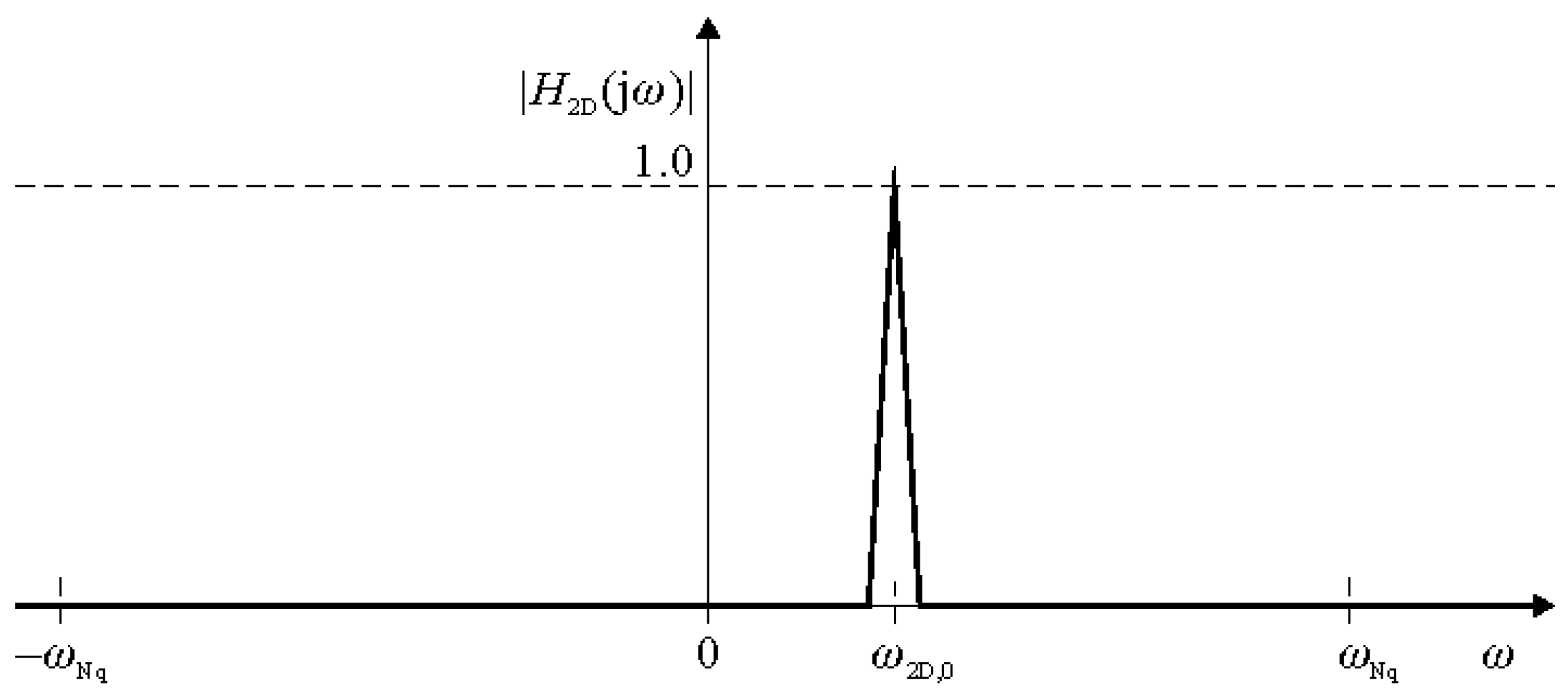
The theoretical magnitude part of a transmittance of the FIR filter used in the method is shown in Figure 1. It provides very effective filtration of the input signal, depending on the removal of higher harmonics, high-frequency components, and DC from this signal. The frequency is denoted as ${\omega }_{2\mathrm{D},0}$ is the filter’s centre frequency, which should be equal to an assumed fundamental frequency of the input (measured) signal, whereas the frequency denoted as ${\omega }_{\mathrm{Nq}}$ is the Nyquist frequency of the measurement path of the signal processing system.

The function shown in Figure 1 is not mathematically an even function. Thus, in light of the signal theory, its implementation requires a two-dimensional filter, whose pulse response is a complex function of time [27,28]. So, the filter response consists of a pair of signals, which is crucial for the operation of the presented algorithm.

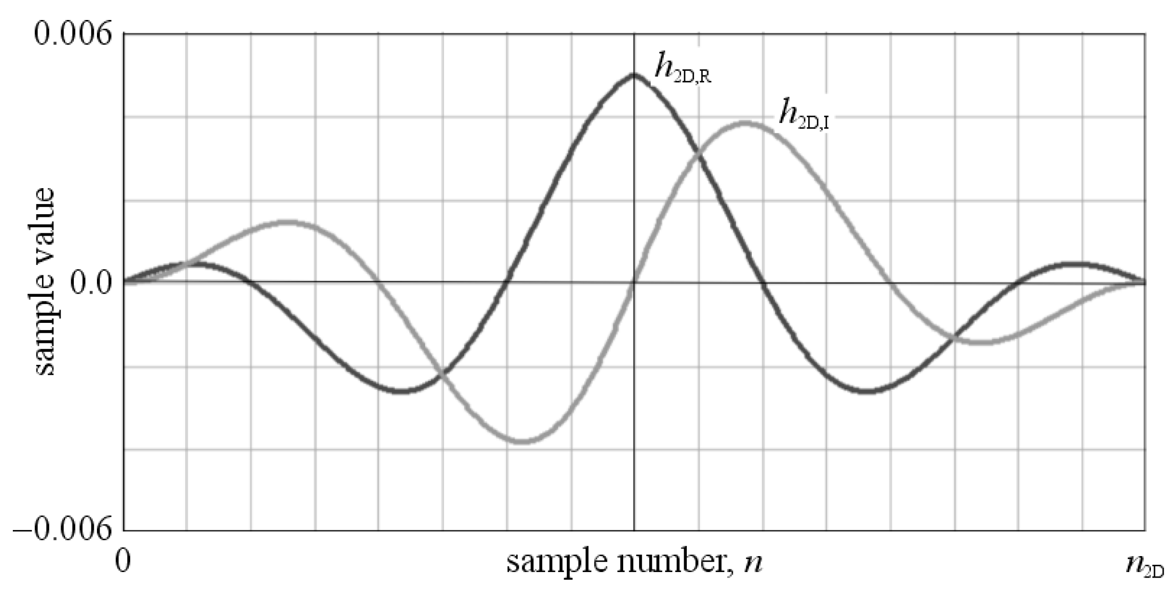
The generalised formula of the filter pulse response is given by the following equation, the inverse Fourier transformation, where $h_{2\mathrm{D},\mathrm{R}}\left(t\right)$ and $h_{2\mathrm{D},\mathrm{I}}\left(t\right)$ are the real and imaginary parts of the response, respectively [27,28,29]:

$$h_{2\mathrm{D}}\left(t\right)=\frac{1}{2\pi }{\displaystyle \underset{-{\omega }_{\mathrm{Nq}}}{\overset{{\omega }_{\mathrm{Nq}}}{\int }}{H}_{2\mathrm{D}}\left(\mathrm{j}\omega \right)e^{\mathrm{j}\omega t}\mathrm{d}\omega }=\frac{1}{2\pi }{\displaystyle \underset{-{\omega }_{\mathrm{Nq}}}{\overset{{\omega }_{\mathrm{Nq}}}{\int }}{H}_{2\mathrm{D}}\left(\mathrm{j}\omega \right)\cos \left(\omega t\right)\mathrm{d}\omega }+\mathrm{j}\frac{1}{2\pi }{\displaystyle \underset{-{\omega }_{\mathrm{Nq}}}{\overset{{\omega }_{\mathrm{Nq}}}{\int }}{H}_{2\mathrm{D}}\left(\mathrm{j}\omega \right)\sin \left(\omega t\right)\mathrm{d}\omega }=h_{2\mathrm{D},\mathrm{R}}\left(t\right)+\mathrm{j}{h}_{2\mathrm{D},\mathrm{I}}\left(t\right).$$

(2)

Assuming temporarily that the following assumption is true:

$${\omega }_{\mathrm{s}}={\omega }_{2\mathrm{D},0}\wedge s_{\mathrm{t}}\left(t\right)\equiv 0,$$

(3)

the signal at the filter’s output will consist of two orthogonal components, in the form of $\sin \left({\omega }_{\mathrm{s}}t\right)$ and $\cos \left({\omega }_{\mathrm{s}}t\right)$ functions. These signals are directly used by the identification algorithm, forming the basis of its operation in the time domain.

Considering the aforementioned assumptions regarding the filter topology, the instantaneous frequency of signals at its output ($f_{\mathrm{s},\mathrm{ID}}$) can be determined based on the following relationship [27,29]:

$$f_{\mathrm{s},\mathrm{ID}}\left(t\right)=\frac{1}{2\pi }{\omega }_{\mathrm{s},\mathrm{ID}}\left(t\right)=\frac{1}{2\pi }\frac{\mathrm{d}}{\mathrm{d}t}{\Phi }_{\mathrm{s},\mathrm{ID}}\left(t\right),$$

(4)

where [27,29]

$${\Phi }_{\mathrm{s},\mathrm{ID}}\left(t\right)=\mathrm{atan}\left[\frac{s_{2\mathrm{D},\mathrm{I}}\left(t\right)}{s_{2\mathrm{D},\mathrm{R}}\left(t\right)}\right]=\mathrm{atan}\left[\frac{S_{2\mathrm{D},\mathrm{I},1}\left(t\right)\sin \left({\omega }_{\mathrm{s}}t\right)}{S_{2\mathrm{D},\mathrm{R},1}\left(t\right)\cos \left({\omega }_{\mathrm{s}}t\right)}\right],$$

(5)

whereby $s_{2\mathrm{D},\mathrm{R}}\left(t\right)$ and $s_{2\mathrm{D},\mathrm{I}}\left(t\right)$ are the filter output signals, and $S_{2\mathrm{D},\mathrm{R},1}\left(t\right)$ and $S_{2\mathrm{D},\mathrm{I},1}\left(t\right)$ are the amplitudes of these signals; in general, both amplitudes are also the functions of time.

In the steady-state of the filter input signal, the amplitudes of both output signals are equal to each other at any time. Therefore, the amplitude of the fundamental harmonics of the input signal is defined formally by the following formula [27,29]:

$$S_{1,\mathrm{ID}}\left(t\right)=\sqrt{{\left[S_{2\mathrm{D},\mathrm{R},1}\left(t\right)\cos \left({\omega }_{\mathrm{s}}t\right)\right]}^2+{\left[S_{2\mathrm{D},\mathrm{I},1}\left(t\right)\sin \left({\omega }_{\mathrm{s}}t\right)\right]}^2},$$

(6)

and $S_{1,\mathrm{ID}}\left(t\right)$ = const.

If the assumptions in Equation (3) are not satisfied, the values calculated based on Equations (4) and (6) are subject to constant and transient measurement error. The value of this error depends on the degree of deformation of the input signal from the sine wave since the output signals are no longer mono-harmonics functions of time. However, since the value of the gain of the filter transfer function decreases with the square of the function of frequency, only low-frequency harmonics are important for the accuracy of the measurement. Also, if Equation (3) is not satisfied, the 2D-FIR output signals are burdened with phase errors—concerning the input signal. The values of the measurement errors are estimated in the next section of this work, devoted to laboratory tests of the presented algorithm.

3. Implementation of the Algorithm

3.1. Selection of the Transfer Function of 2D-FIR

The theoretically existing transfer function of the 2D-FIR, which is shown in Figure 1, is band-limited. As a result, the length of its pulse response tends to infinity [27,28,29]. Thus, in the presented algorithm, the 2D-FIR filter with modified transfer function was applied, to pre-process the analysed signal, whose magnitude part is given by Equation (7), where $N_{\mathrm{IDF}}$ is the function’s parameter and $N_{\mathrm{IDF}}$ = 2.

$$\left|H_{2\mathrm{D}}(\mathrm{j}\omega )\right|={\left|\left[\frac{\sin \left(\pi \frac{(\omega -{\omega }_{2\mathrm{D},0})}{{\omega }_{2\mathrm{D},0}}\right)}{\pi \frac{(\omega -{\omega }_{2\mathrm{D},0})}{{\omega }_{2\mathrm{D},0}}}\right]\right|}^{N_{\mathrm{IDF}}}={\left|\mathrm{Sa}\left[\pi \frac{(\omega -{\omega }_{2\mathrm{D},0})}{{\omega }_{2\mathrm{D},0}}\right]\right|}^{N_{\mathrm{IDF}}}.$$

(7)

The function has been selected as a result of extensive studies of the algorithm as a good compromise between the effectiveness of attenuating the selected input signal’s components, i.e., the assumed precision of the IA operating, and the length of the filter response. The length of the 2D-FIR response should be as short as possible because it directly affects the value of the delay of the input signal processing. It is very critical for the quality of the identification process, which should be done with the shortest possible delay.

The filter with such transfer function also provides effective filtration of the input signal when the value of the input delay is minor. The plot of the function given by Equation (7), when $N_{\mathrm{IDF}}$ = 2, is shown in Figure 2.

A discrete-time implementation of Equation (7), when $N_{\mathrm{IDF}}$ = 2, is described by Equations (8) and (9), defining the real and imaginary parts of the pulse response of the 2D-FIR, respectively [27,28,29]:

$$h_{2\mathrm{D},\mathrm{R}}\left(n\right)=\frac{1}{k_{\max }}{\displaystyle \sum _{k=-k_{\max }}^{k_{\max }}{\mathrm{Sa}}^2\left[\pi \frac{(\frac{k}{k_{\max }}{\omega }_{\mathrm{Nq}}-{\omega }_{2\mathrm{D},0})}{{\omega }_{2\mathrm{D},0}}\right]}\cos \left(\pi \frac{k}{k_{\max }}n\right):n=0,1,\dots ,n_{2\mathrm{D}},$$

(8)

$$h_{2\mathrm{D},\mathrm{I}}\left(n\right)=\frac{1}{k_{\max }}{\displaystyle \sum _{k=-k_{\max }}^{k_{\max }}{\mathrm{Sa}}^2\left[\pi \frac{(\frac{k}{k_{\max }}{\omega }_{\mathrm{Nq}}-{\omega }_{2\mathrm{D},0})}{{\omega }_{2\mathrm{D},0}}\right]}\sin \left(\pi \frac{k}{k_{\max }}n\right):n=0,1,\dots ,n_{2\mathrm{D}},$$

(9)

where $n_{2\mathrm{D}}$ is the filter order, $n$ is the sample number, and $k_{\max }$ is the number of points analysed on the frequency characteristic of the filter, in the range of $\langle -{\omega }_{\mathrm{Nq}},{\omega }_{\mathrm{Nq}}\rangle$.

To accurately map the assumed transfer function of the 2D-FIR, the required filter order is as follows [27,28,29]:

$$n_{2\mathrm{D}}=2\frac{{\omega }_{\mathrm{smp}}}{{\omega }_{2\mathrm{D},0}}+1\wedge n_{2\mathrm{D}}\in {\rm N},$$

(10)

where ${\omega }_{\mathrm{smp}}$ is the signal sampling frequency.

Figure 3 shows plots of the components of the 2D-FIR filter pulse response, defined by Equations (8) and (9).

Taking Equation (10) into account, the filtering algorithm introduces the average delay (${\tau }_{2\mathrm{D}}$) of both output signals, in relation to the input signal, which is as follows [27,28,29]:

$${\tau }_{2\mathrm{D}}=n_{2\mathrm{D}}\frac{2\pi }{{\omega }_{\mathrm{smp}}}.$$

(11)

3.2. Structure of the Identification Algorithm

The block diagram of the identification algorithm is shown in Figure 4.

The algorithm consists of the following functional blocks:

• DF: This is an FIR decimation filter [30] (an optional block) whose role is explained in the last section of the work.
• 2D-FIR: An FIR-type filter, with the aforementioned transfer function. This task is realised in the “Real” and “Imag” sub-blocks of 2D-FIR.
• AFB: This block consists of two sub-blocks (A and F) and computes the frequency and amplitude of the basic harmonics of the input signal; also, the AFB generates the grid voltage-synchronous signal, which can be used in the control block of the power electronics (or other) devices.

The basis of the AFB operation is the formulas given by Equations (4) and (6), whereas the synchronisation signal ($s_{\mathrm{SYNC}}$) is generated based on both $s_{2\mathrm{D},\mathrm{I}}$ and $S_{1,\mathrm{ID}}$. Assuming that Equation (3) is true, the 2D-FIR output signal ($s_{2\mathrm{D},\mathrm{I}}$), coming from its “Imag” sub-block, is in-phase with the input signal ($s$). The amplitude of the $s_{2\mathrm{D},\mathrm{I}}$ is then normalised by multiplying it by the output signal of the “$x^{-1}$” block, which computes the reciprocal value of the $S_{1,\mathrm{ID}}$. As a result, the grid voltage-synchronous signal has, at any time, a unity value of amplitude and is in phase with the basic harmonics of the input signal: $s_{\mathrm{SYNC}}\left(t\right)=\sin \left({\omega }_{\mathrm{s}}t\right)$.

3.3. Arrangement of the Laboratory Stand

The presented algorithm was implemented in the digital signal processor (DSP) based evaluation board (EvalBoard), type ALS-G3-1369 [31], with a floating-point DSP, type ADSP-21369, the SHARC^® family of Analog Devices Inc. [32,33]. This board is hereinafter referred to as the “Identification System” (IS). The general view of the laboratory stand, during tests, is shown in Figure 5.

This board, among others, is equipped with a multi-channel precision AD converter with simultaneous sampling capability and TRUE-BIPOLAR type inputs, as well as a multi-channel DA converter with outputs that are also of a TRUE-BIPOLAR type. This system is intended for use in advanced measurement applications as well as for the implementation of complex control algorithms of power electronics devices, e.g., [23,24,25,26]. Potentially, it offers significant computational power, up to 2400 MFLOPS (million-floating-point operations-per-second), if the math units operate in a single-instruction-multiple-data (SIMD) mode [31]. The ADSP-213xx family of DSP supports SIMD operations, which, under certain conditions, double the computational rate over ADSP-2106x (single-instruction-single-data, SISD) processors. The DSP run-time library, for ADSP-213xx processors, makes extensive use of their SIMD capabilities, and it has been implemented in the IA. So, the 2D-FIR filtration algorithm is realised in the SIMD mode of operation of the mathematical units of the processor, using 2-dimensional (vector) processing of the input signal. The filtration algorithm is based on the following functions: “Fir_mccoeff.asm”, which is a multi-channel FIR implementation [33], “fir()”, and “*fir()”. The last two functions are available in the C-compiler run-time library for SHARC^® processors [30].

To verify the values of the delays and measurement errors introduced by the identification algorithm, tests were carried out for the measured signal with different degrees of its non-linear distortion ($THD$), deviations from the default frequency, and magnitude changes. The tests referred to the measured signal with the assumed value of its basic frequency as in the European power grid (50 Hz). The changes in this frequency were close to the normative value [34] as well as significantly exceeding it. The tests were also carried out under the following conditions: strong deformations of the measured signal (value of its $THD$ up to 30%, including up to 13 first harmonics), the presence of DC in the signal, and the presence of high-frequency components in the signal. The tests were conducted for the values of the parameters of IA:

$$f_{\mathrm{smp}}=\frac{1}{2\pi }{\omega }_{\mathrm{smp}}=20\mathrm{kHz},n_{2\mathrm{D}}=801.$$

(12)

4. Results

The waveforms shown in the following figures were obtained using two methods, the PLOT function of the VisualDSP++, a development environment for Analog Devices Inc. signal processors [35], which allows for visualisation of numerical data, stored in arrays, or with the use of the DA converter and digital oscilloscope. The measured signal was generated using the digital synthesis method, allowing for a free setting of almost all of its parameters. Also, the source of the signal was the power line or, in some cases, the signal came from the external generator.

In Figure 6 sample waveforms of the signals in the IS as shown, as follows: signal at the input of the 2D-FIR ($s$), signals at the output of the 2D-FIR ($s_{2\mathrm{D},\mathrm{R}}$, $s_{2\mathrm{D},\mathrm{I}}$), and the calculated instantaneous amplitude’s value of the fundamental harmonics of the input signal ($S_{1,\mathrm{ID}}$). The frequency of the input signal was approx. equal to 50 Hz, i.e., the centre frequency of the 2D-FIR.

Figure 7 and Figure 8 show the selected waveforms in the IS, concerning the most characteristic cases of the measured signal shape and changes in the values of its parameters over time. These waveforms are the following: the input signal ($S$), the actual frequency of the input signal ($f_{\mathrm{s}}$), the input signal’s frequency, calculated by the algorithm ($f_{\mathrm{s},\mathrm{ID}}$), the actual amplitude of the basic harmonics of the input signal ($S_1$), and the amplitude of the basic harmonics of the input signal, calculated by the algorithm ($s_{1,\mathrm{ID}}$).

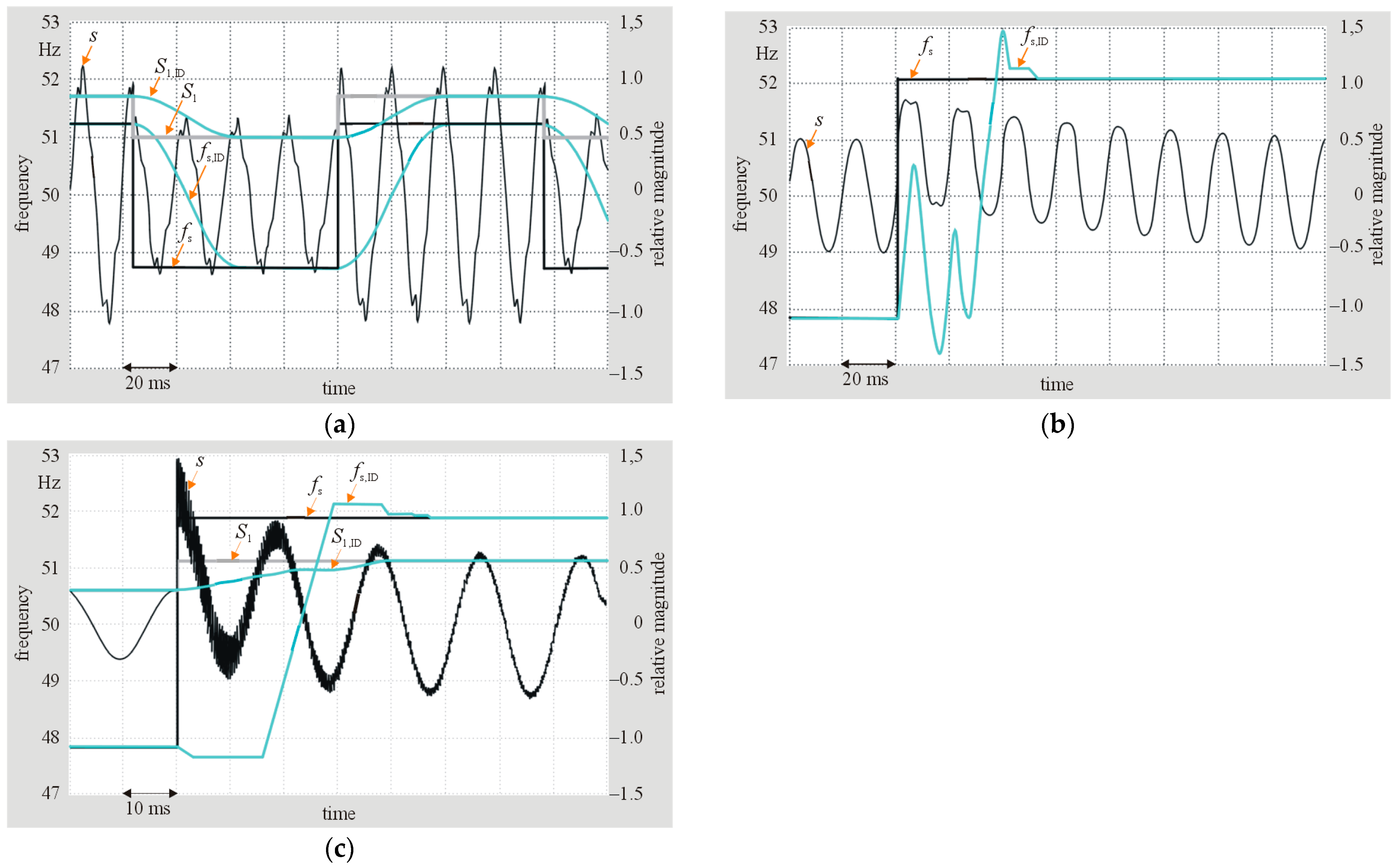
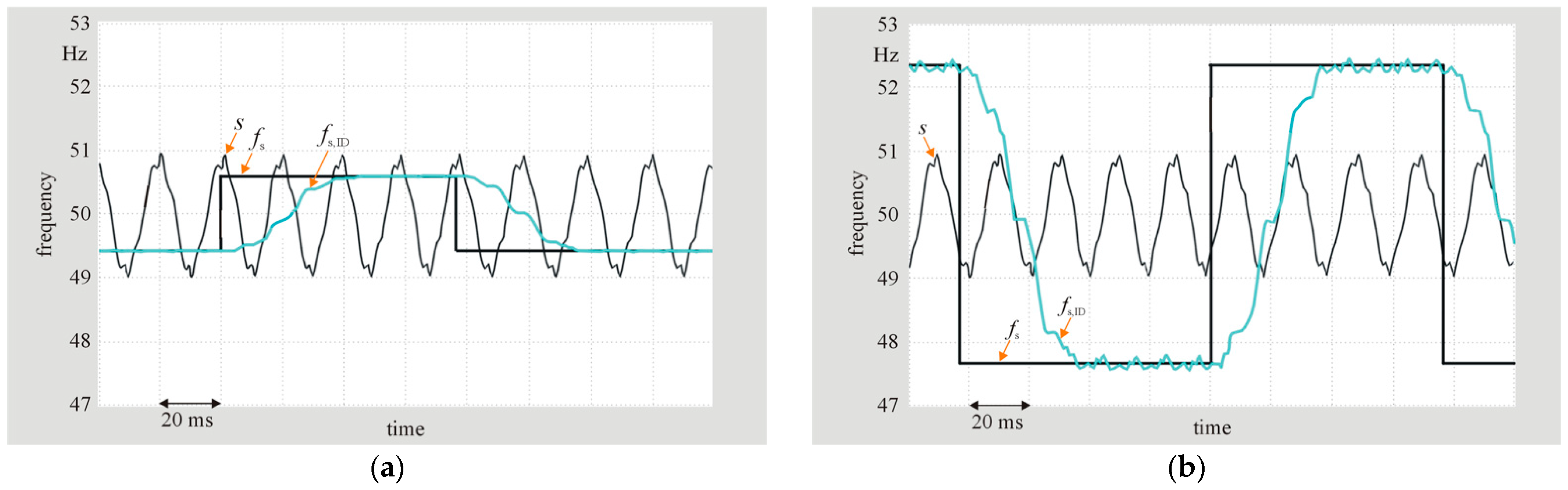
In particular, Figure 7 shows the results of the algorithm tests for the strongly deformed measured signal ($THD$ = 30%), with a constant magnitude of this signal and a step-change, with two different values, in its frequency.

In turn, Figure 8 presents the results of the algorithm tests under the following conditions: a step-change of a magnitude of the measured signal, the presence of the transient component in this measured signal, and the presence of a high-frequency component in the measured signal. Therefore, the waveforms shown in Figure 8 refer to the following exemplary parameters of the measured signal, which significantly exceed the normative values:

• $THD$ = 30% and a step-change in both the amplitude of the input signal and its frequency,
• the measured signal contains an exponential-type transition component with an initial amplitude equal to 80% of the basic harmonics of the signal, a time constant of 100 ms, and an attenuated 3-harmonics,
• the measured signal with an attenuated amplitude of its basic harmonics and presence of the transient component with an initial amplitude of about 100% of the basic harmonics, as well as with the presence of the attenuated high-frequency (1.5 kHz) component in the form of a rectangular waveform with a time constant of 60 ms.

In the following part of the section the laboratory experiments, related to the DC power supply with parallel reactive and distortion power compensation function (PFC—Power Factor Correction) [25], are presented. In the case of this device, due to the inverter control needs, it is also necessary to obtain the sine wave, grid voltage-synchronous signal.

These tests were conducted for a number of loads, both linear and nonlinear, connected to the same grid node as the power supply. However, only waveforms associated with one of the most critical, for the effective operation of this device with kinds of loads, are presented in the figure; these are thyristor voltage regulator, loaded by R, and the same regulator, loaded by R-L. The firing angle of the thyristor in both cases was set at 90 electrical degrees.

In Figure 9, the following waveforms are presented: grid voltage ($s$), sine wave, grid voltage-synchronous signal ($s_{\mathrm{SYNC}}$)—at the output of the IA, and load current.

5. Discussion

In the first part of the tests, only the deviation of the frequency in the signal was taken into account; it was equal to ±0.7 Hz and ±2.3 Hz. In the first case, the maximum instantaneous value of the signal frequency identification error was equal to ±0.02%, while in the second case, this value was equal to ±0.2%. Thus, as expected, the research on the presented identification algorithm proves, first of all, the dependence of the measurement error value on the deviation of the measured signal frequency from the centre frequency of the 2D-FIR filter. This error increases in the case of strong deformation of the measured signal. For signals with small values of $THD$, i.e., less than approx. 10%, or for signals being strongly deformed but with a frequency close to the centre frequency of the 2D-FIR, the IS generates aperiodic and fixed over time output signals ($f_{\mathrm{s},\mathrm{ID}}$, $S_{1,\mathrm{ID}}$).

The proposed algorithm is highly resistant to the presence of transient components in the measured signal, including those with high amplitudes concerning the basic component of the measured (input) signal. For the measured signal with a $THD$ not exceeding 10%, the values of the relative measurement errors were within the range of 0.05–0.1%, in relation to the actual frequency of the measured signal as well as to the amplitude of its basic harmonics. When the frequency of this signal coincides with the 2D-FIR filter centre frequency, the values of the identification errors do not exceed the errors associated with the AD conversion process, even for a strongly distorted measured signal.

The generated by the IA synchronous signal ($s_{\mathrm{SYNC}}$) is in-phase with the input signal. The value of error, related to the amplitude of $s_{\mathrm{SYNC}}$, is below 0.05%, while the value of the phase error is in the range of ±2 electrical degrees—for typical conditions of the grid operation [34].

The response time of the IS is consistent with the aforementioned indicated value of the length of the 2D-FIR filter pulse response, i.e., it does not exceed 2 periods of the input signal.

6. Conclusions

Research on the identification algorithm shows that, for real waveforms, e.g., a voltage in the power grid, for normative deviations in the measured signal frequency from its rated value, and for the normative value of the $THD$, the relative measurement errors, concerning both the frequency and the amplitude of the measured signal, did not exceed 0.1%. This means that frequency measurement has an effective resolution better than 0.05 Hz. When the frequency of the measured signal coincides with the 2D-FIR filter centre frequency, the values of the identification errors do not exceed the errors associated with the AD conversion process. It is a result of the applied FIR filter transfer function that gives the algorithm exceptional resistance to the presence of higher harmonics or DC component in the measured signal.

The delay value of the identification process is short and corresponds to about two periods of the measured signal. An additional advantage of the algorithm is the relatively small demand for computational power and the possibility of directly using a processor math unit in the SIMD mode—for the realisation of a two-dimensional FIR filter algorithm. In this context, for the values of the operational parameters of the identification algorithm given in this work, its execution time was about 2.8 μs (assuming a processor core clock frequency of 360 MHz), i.e., approximately 5.6% of the time available to the interrupt service routine. However, if the required sampling rate is significantly higher than specified in Section 3, the required computational power of the system will also increase significantly. The reason for this, among others, is the need to increase the 2D-FIR filter order. In this case, a decimation filter (DF) can be applied at the identification algorithm input, which allows for lowering the effective signal sampling rate to the desired value. Thus, the developed algorithm is instant, precise, and easy to implement in processors or micro-controllers. Moreover, the needed computational power can be easily scalable by changing the decimation factor of the DF.

Although the IA is related to cooperation with the power grid, it can be used with other signal sources, assuming that the default values of the frequency of these signals are known.

The disadvantage of the identification method is the need to know the default frequency of the measured signal. However, in the presented application of the IA, this is of marginal importance.