Abstract
The negative impact of the displacement currents on the operation of electromagnetic converters results in additional losses and faster insulation degradation, as well as the self-resonance phenomenon. Effective measurement of the dielectric displacement currents in converters is quite complex; thus, advanced simulation programs should be used. However, currently, they do not enable the analysis of the systems in terms of the displacement currents distribution. In order to elaborate an effective tool for analyzing the distribution of the displacement currents by means of the Finite Element Method, we have decided to supplement the well-known reluctance-conductance network model with an additional capacitance model. In the paper, equations for the linked reluctance-conductance-capacitance network model have been presented and discussed in detail. Moreover, we introduce in the algorithm the Harmonic Balance Finite Element Method (HBFEM) and the Fixed-Point Method. This approach enables us to create a field model of electromagnetic converters, which includes the electromagnetic core’s saturation effect. The application of these methods for the reluctance-conductance-capacitance model of the finite element has allowed us to develop a practical tool ensuring complex analysis of the magnetic flux, eddy, and the displacement currents’ distribution in electromagnetic converters with an axial symmetrical structure.
1. Introduction
The process of miniaturization of electronics systems, which has been observed for over 20 years in electrical engineering and electronics, has resulted in many designers creating new prototypes, striving for their continuous miniaturization while maintaining both sufficiently high power and efficiency. The miniaturization of modern electrical devices, particularly electromagnetic converters, would not be possible without the development of new types of magnetic materials [1,2], but primarily without the development of power electronics and the increase in the frequency of the power sources of the converters [3,4]. By increasing the frequency of the source, the designers have been able to develop new types of electromagnetic converters that operate with frequencies reaching tens or hundreds of kilohertz (kHz), such as medium- and high-frequency transformers operating in Dual Active Bridge (DAB) systems, as well as systems that are already capable of operating at frequencies up to tens of megahertz (MHz), i.e., Wireless Power Transmission (WTP) systems [5,6,7]. Currently, a few attempts can be observed to develop electromagnetic converters, of which the operation is based on the use of not only the conductivity currents but also the dielectric displacement currents, for example the high-frequency capacitive-inductive transformer developed by the team of Prof. J. Starzyński from the Military University of Technology in Warsaw [8].
The impact of the dielectric displacement currents on the electromagnetic field distribution can already be observed in converters supplied by voltages of frequencies of several dozen kilohertz. The effect is particularly significant in the area of the core made of a composite material or the ferrite itself, between the winding conductors, as well as in the conductor insulation itself.
While conducting our research on the design of electromagnetic converters, we have studied multiple open literature positions and noticed that there are a few works discussing methods that enable the analysis of distribution of the displacement and eddy currents in electromagnetic converters [9,10,11,12,13]. However, none of these enable the detailed time-domain analysis using a multistage approach of the Finite Element Method (FEM). Moreover, it can be noticed that in the available commercial software for the field analysis of electromagnetic phenomena, there are no tools that would allow for a time-domain analysis of a dielectric displacement current effect.
This article is the first in a series, in which we would like to present the results of their research related to the development and implementation of two- (2D) and three-dimensional (3D) numerical field models enabling the analysis of the operating states of electromagnetic devices and converters. Apart from the eddy currents, the impact of the dielectric displacement currents on the electromagnetic field distribution has been included. In this article, we will present the results of the research related to the development of a 2D field model of the inductor with an axisymmetric structure (see Figure 1), which includes the impact of the dielectric displacement currents and eddy currents in the area of the ferrite core. In this study, the displacement current effect in the winding area has not been considered. As is well known, ferrite is a magnetic material produced by sintering powdered-metal oxides. According to the hypothesis of E. Blechschmidt, the simplified ferrite microstructure can be considered as shown in Figure 2. The dark gray circles represent conductive magnetic particles (commonly called grains), while the light gray region (the region between grains) is considered as an area representing capacitance and leakage related to ferrite insulation. Thus, apart from remaining an ability to concentrate the magnetic flux (high value of magnetic permeance) and a high value of resistivity limiting the influence of eddy current losses, a magnetic material will also have dielectric properties. Due to the latter property, placing ferrite in the area of the electromagnetic field of a sufficiently high-frequency value will result in ferrite losses generated by the induction of the eddy currents as well as the dielectric displacement currents. In order to analyze the electromagnetic field distribution with the contribution of the dielectric displacement currents in the considered inductor system (see, Figure 1), we have applied a 2D approach to the edge element method (EEM) [14,15,16] using the A-V-T0 formulation. The inductor model discussed in the paper consisted of two TI-M fittings made of ferrite and a winding. To solve the obtained EE equations, we implemented the Harmonic Balance Method combined with the Fixed-Point Method [17,18,19,20,21]. Moreover, the work presents both the magnetic flux and the eddy current densities distributions as well as the dielectric displacement current density for the selected time samples in the core of the considered inductor. As a supplement to the obtained distribution diagrams, the waveforms of the discussed magnitudes for three selected discretization mesh elements have also been presented.
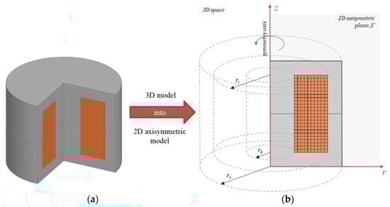
Figure 1.
3D view of a considered inductor (a) and its representation in a 2D axial symmetry system (b).

Figure 2.
Microstructures of ferrite and the equivalent circuit diagram of the magnetic and electric properties: (a) simplified microstructures and schematic of ferrite, (b) inductance-resistance model, (c) capacitance-resistance model [14,15].
2. Edge Element Model of Inductor/Choke Using HBM
In this paper, to analysis of the electromagnetic field, the 2D approach to an Edge Element Method has been applied. In the used approach, the magnetic field distribution is described by the edge values of the vector potential A, i.e., by a magnitude that has been calculated based on the integral of the values of an A potential along the edge of the finite element [22]. In determining the distributions of both the eddy and displacement currents induced in the massive ferrite core, we have used the relationship between the current density vector J, vector magnetic potential A, and the gradient of the scalar electric potential V (∇V) [23]:
where σ and ε represent the electrical conductivity and dielectric permittivity of medium, respectively. In the discussed axisymmetric system, both the displacement and eddy currents states closed current loops (Figure 3); thus, a voltage drop (potential difference V) on branches representing these loops must be equal to zero ∇V = 0 [24]. Moreover, in this paper, the source currents distribution has been determined by means of the vector electric potential T0 (i.e., J = rotT0) [25,26].
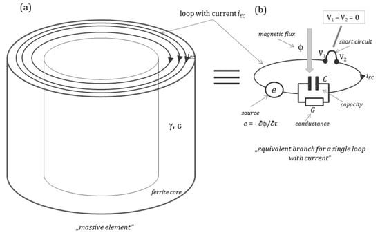
Figure 3.
Massive element with loop currents (a) and the equivalent branch for a single loop with a current (b).
In the applied approach, EE equations describing the distribution of A potential edge values are equivalent to loop equations of the reluctance network model (RN), which already has been proved [27]. Figure 4 shows the fragment of a 2D reluctance network model for a single loop. The location of branch reluctances and branch magnetomotive forces (mmfs) has been marked in the loop. For the 2D EE system, the equations describing the magnetic field distribution in the considered inductor can be written as follows:
where the product of loop matrices and as well as matrix of the branch reluctances Rµg represents the loop reluctance matrix, i.e., matrix Rµo [28], is the vector of the edge values of potential A (i.e., loop fluxes of 2D RN) [22]; and Θg is the vector of branch magnetomotive forces (mmfs). The product of the transposed loop matrix and the branch magnetomotive forces Θg represents the vector of loop magnetomotive forces Θ(mmfs). In the elaborated algorithm, the loop mmfs vector consists of three components, i.e., (a) the Θ0 component representing loops mmfs in the region of conductive currents flowing through the coil; (b) the ΘEC component describing the loops mmfs related to the induced eddy currents in the region of ferrite core; (c) the ΘDC component representing the loop mmfs related to induced displacements currents in the region of the ferrite core. In the research, the magnetic field sources related to the winding region, i.e., the loop mmf Θ0, have been calculated with an application of the T0 approach, i.e., Equation (3), which uses the electric vector potential T0 with the determined direction of the current density vector for the electromagnetic field description:

Figure 4.
2D representation of the reluctance network (RN) for an axial symmetry system.
The component describing magnetic field sources in regions with the eddy currents has been determined based on relationship γ∂A/∂t, which is the product of the ferrite core conductivity γ and the derivative of magnetic vector potential A, which in the 2D approach has the following form:
whereas the component representing sources in regions with displacement current has been calculated using formula ∂∂t (ε∂A/∂t), which is the derivative of the product of the dielectric permittivity of the core ε and a derivative of the magnetic vector potential A. The equation for the discussed approach has the following form:
where N is matrix that transpose the values in loops around edges to the values in loops that are ordered to centers of the element faces [14], the matrix zk represents the coil turns agreement in the edge element space-matrix zk and is also used to determine of fluxes linked with coil and electromotive forces (emfs) [29]; and ic describes the value of the current in the system coil. The symbol represents the vector of the eddy currents assigned to the appropriate edges of CCN (see, Figure 4 and Figure 5), whereas constitutes the vector of the dielectric displacement currents of the CCN (see, Figure 4 and Figure 5). The matrix G and matrix C, which occur in Formulas (4a) and (4b), respectively, represent the matrix of the branch conductances and matrix of the branch capacitance of one-dimensional (1D) Conductive-Capacitive Network (CCN) coupled with 2D Reluctance Network. In the proposed approach, the coupling between both network models has been conducted by the sources. In case of magnetic field, i.e., for the reluctance network model, field sources are identified by the eddy currents as well as the dielectric displacement currents , whereas for the conductance-capacitance network model, field sources are identified on the basis of loop magnetic fluxes . The form of the implementation of coupling between the Reluctance Network and Conductive-Capacitive Network has been illustrated in Figure 5.
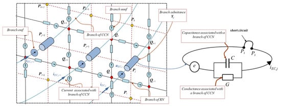
Figure 5.
Fragment of the 2D Reluctance Network (RN) coupled with the 1D Conductive-Capacitive Network (CCN).
In the applied 2D approach of EEM, the values of the branch reluctances of the RN are found using the following integral:
whereas the branch conductances and capacitors of CCN are determined on the basis of the branch conductances and branch capacitors of edge element on the basis of the following relations:
In which branch conductances Gg and capacitors Cg of the edge element are calculated applying the following integrals:
where wfi and wfj are the facet function of ith and jth facet of the ring element with a rectangular cross-section (see, Figure 5); wei and wej are the edge function of ith and jth of the edge of the ring element; Ve is the volume element; kn is the nodal incident matrix of edge element [14]; and ν, γ and ε are the reluctivity, conductivity and electrical permittivity of the medium, respectively. In the in-house algorithm, the integrals (5) and (7a,b) have been calculated by applying the following formula:
where nw is the node number of the applied elements and fe (Pi) is the value of the integer function in node Pi [14]. It should be noted that Equation (8) [27,30] can be applied to calculate the branch reluctance (6a,b), conductance (6a) and branch capacitance (6b) values of ring elements with rectangular cross-section and enables to obtain the non-coupled models, of which the parameters could be described by the means of the classical equivalent circuits method equations.
Taking into consideration Equations (3), (4a) and (4b), as well as in Equation (2), the EEM Equation will have the following form:
Because the considered system is supplied by the voltage source, the obtained Equation (9) must be completed using the formula describing the electric circuit of an inductor:
where uz represents the supply voltage of the winding, Rc constitutes the resistance of the coil and is the magnetic flux linked with the winding of the considered inductor and determined by the following equation [29]:
Inserting Equation (11) into Equation (10) and combining Equation (10) with Equation (9) enables to create the system of equations describing the distribution of electromagnetic field in the considered inductor:
To solve the formed equation system shown in Equation (12), we have implemented the Harmonic Balance Method (HMB) combined with the Fixed-Point Method. The applied approach has been proposed and discussed in detail by Biro in [17]. In the discussed approach, the v parameter value can be expressed by the sum of two components (13), i.e., vFP and (v-vFP). The first one is directly related to the convergence time of the calculation, whereas the second one represents the considered magnetic circuit’s nonlinear character. According to Equation (13), the loop reluctance matrix Rµo has been converted into the sum of two components (see Equation (14)) as well. The point of the discussed HBM method is an iterative analysis of the system nonlinearity using a Fourier transform, the results of which are applied in further iterations of the calculation process. Particular attention should be paid to the process of determination of the vFP value [19,31]. Based on the open literature research and conducted studies, we applied the solution of the vFP value determination based on Equation (15), which reduces the time consumption by approximately two times:
where v is the magnetic reluctivity and v FP is the fixed-point parameter.
Then, by applying Equation (14) in the system of the electromagnetic field equations formula (12) and introducing the HBM and Fixed-Point method, the following equations system has been elaborated:
where ω is the electrical pulsation of the fundamental harmonic of the supply voltage waveform and m is the order of the considered harmonic, whereas k symbolizes the actual iteration step of the calculation process.
In this paper, the equations system (16) has been solved iteratively. The obtained current values and magnetic flux values in the (k + 1)th iteration has been converted into time-domain waveforms. In order to determine the waveforms of current ic and magnetic flux vector in the (k + 1)th iteration, the following formulas have been used:
where: M is the total number of considered harmonics.
To execute another iteration, the obtained waveforms of currents and fluxes are introduced as parameters to the right-hand side of Equation (16). However, before that, the value of reluctivities vFP and (v-vFP) must be recalculated based on the newly obtained values of magnetic flux , thus correcting the values of loop reluctance matrix Rµo (see Equation (14)). The iteration process is considered as completed when Equation (19) is met:
where δ is the parameter that defines the termination condition.
3. Results
The output of the discussed research is the axisymmetric field model of the electromagnetic converter, i.e., the inductor. Calculations have been conducted for different values of frequency in order to determine the change in amplitude of displacement and eddy current in the frequency domain. Using the elaborated software, we have run a simulation of an electromagnetic field distribution in considered system. The assumed parameters are shown in Table 1.

Table 1.
The field model parameters.
To present the obtained research results, we have determined and compared, using the elaborated field model, the distribution of the magnetic flux, eddy currents and displacement currents in the analyzed inductor for different supply frequencies and voltage shapes. The system has been supplied by the sinusoidal voltage with a frequency of 1 kHz, 10 kHz and 100 kHz and rectangular voltage with a frequency equal to 100 kHz. In the calculation, 30 harmonics have been used for the Harmonic Balance Method in the case of a sinusoidal voltage source and 100 harmonics for a rectangular voltage source. In Figure 6 and Figure 7, the waveforms of the inductor current ic and the flux linkage Ψ for the system supplied from a voltage with a frequency of 1 kHz are shown. In contrast, Figure 8 and Figure 9 present the distributions of the displacement current density and eddy-current density for the selected time samples, on which the waveforms of the displacement currents iDC and eddy currents iEC for the three selected regions of ferrite core have been shown, respectively. For the other frequencies (10 kHz and 100 kHz), we have presented only a distribution diagram of eddy and displacements currents densities and corresponding waveforms in the time domain for three selected points.

Figure 6.
Inductor current ic waveform.

Figure 7.
Coil concentrated flux Ψ waveform.

Figure 8.
Distribution of the displacement current density in the ferrite core for time t = 0.92 ms (a) and the waveforms of the displacement currents iDC for three selected points of ferrite core (b) for a frequency of 1 kHz.
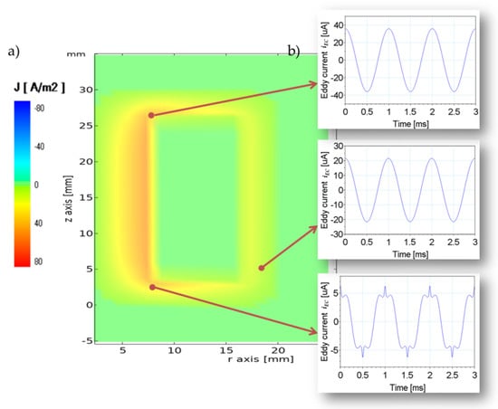
Figure 9.
Distribution of the eddy current density in the ferrite core for time t =1 ms (a) and the waveforms of the eddy currents iEC for three selected points of ferrite core (b) for a frequency of 1 kHz.
In Figure 6, the impact of the core saturation can be observed. The current waveform for this case is distorted and mainly includes the harmonics of the 3rd, 5th and 7th order. The waveform of the flux linkage is sinusoidal. Similar to the flux, the waveforms of the eddy current and displacement current, shown in Figure 8 and Figure 9, respectively, also keep their sinusoidal shapes. However, a certain deviation in the waveforms of both currents can be observed in regions at the bottom, due to the symmetry of the system at the top of the middle column. Figure 10 presents the distribution of the magnetic flux density. What is characteristic is that the saturation impact on the magnetic flux can be observed mainly in the inner corners of the core.

Figure 10.
Magnetic flux density B distribution in the considered inductor for t = 0.25 ms for a frequency of 1 kHz.
Figure 11, Figure 12, Figure 13 and Figure 14 present the distribution diagrams of the eddy and displacement currents in the ferrite core. Diagrams have been supplemented by the time-domain waveforms of corresponding magnitudes for three selected points of the mesh. In Figure 12 and Figure 14, the proportional increase in the amplitude of the displacement current to frequency can be observed. Similar to Figure 8, the current observed at the bottom region of the core is distorted. However, the distortion decreases with the increase of the source frequency. In contrast to a displacement current, amplitudes of the eddy currents in the selected points have very similar values for each source frequency. According to Equation (12), an eddy current is proportional to the derivative and, thus, to both emf and voltage uz.

Figure 11.
Distribution of the eddy current density in the ferrite core for time t = 100 us (a) and the waveforms of the eddy currents iEC for three selected points of ferrite core (b) for a frequency of 1 kHz.

Figure 12.
Distribution of the displacement current density in the ferrite core for time t = 70 us (a) and the waveforms of the displacement currents iDC for three selected points of ferrite core (b) for a frequency of 1 kHz.

Figure 13.
Distribution of the eddy current density in the ferrite core for time t = 10 us (a) and the waveforms of the eddy currents iEC for three selected points of ferrite core (b) for a frequency of 100 kHz.

Figure 14.
Distribution of the displacement current density in the ferrite core for time t = 7 us (a) and the waveforms of the displacement currents iDC for three selected points of ferrite core (b) for a frequency of 100 kHz.
Although the studied frequencies are high, the displacement current’s amplitudes values are relatively small and could be neglected in practical applications. However, converters that operate with frequencies from the range of kHz are hardly ever supplied by sinusoidal voltage. Instead, they are often fed by a trapezoidal or rectangular wave. In Figure 15, Figure 16, Figure 17 and Figure 18, the waveforms of the inductor current, flux linkage as well as the eddy and displacement currents in a selected element for the case with a rectangular voltage source of 100 kHz have been presented, respectively. Figure 17 and Figure 18 are also supplemented with distribution diagrams of the eddy current density and displacement current density, respectively. In Figure 18, peaks of significant amplitude can be observed, and in comparison to Figure 14, the amplitude of the displacement current is much higher than in the case of a sinusoidal voltage source. Moreover, the waveforms for the considered voltage sources differ significantly from one another. In the case of a sinusoidal voltage source, the displacement and eddy current waveform, as well as emf, flux linkage and inductor current waveforms, are also sinusoidal, whereas for the rectangular voltage source, the waveform of the displacement current is composed of periodic peaks. Both the flux linkage and inductor current waveforms are triangular, while emf and eddy current waveforms are rectangular. The specified shape of displacement current waveform results from a steep slope of emf. A value of displacement current associated with a branch of a finite element is proportional to the first-degree derivative of the branch emf ϑue/ϑt and the second-degree derivative of the loop magnetic flux associated with an edge value of the element ϑ2φ/ϑt2. On the basis of obtained results, it could be concluded that the displacement currents of the highest values will be induced in systems fed by a rectangular voltage.

Figure 15.
Inductor current ic waveform for the case with a rectangular voltage source.

Figure 16.
Coil concentrated flux Ψ waveform for the case with a rectangular voltage source.

Figure 17.
Distribution of the eddy current density in the ferrite core for time t = 9 us (a) and the waveforms of the eddy currents for three selected points of ferrite core (b) for a frequency of 100 kHz.
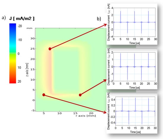
Figure 18.
Distribution of the displacement current density in the ferrite core for time t = 5 us (a) and the waveforms of the displacement currents for three selected points of ferrite core (b) for a frequency of 100 kHz.
4. Results Validation
The validity of the obtained results has been verified by means of Comsol Multiphysics software. The simulation was done on a field model of the electromagnetic inductor and concerned the distribution and waveforms of the magnetic flux density and coil concentrated flux, as well as the induced currents i.e., the eddy and dielectric displacement currents. Both the conditions and the numerical model regarding the dimensions and applied materials for conducted studies and verification simulation are the same. In the COMSOL simulation, the axisymmetric model with a triangular mesh has been used. For the calculation, the magnetic field and electric circuit formulation have been used. The results obtained for the sine wave with a frequency equal to 1 kHz are shown in Figure 19, Figure 20 and Figure 21.

Figure 19.
(a) Inductor current ic waveforms for the case of a sinusoidal voltage source and frequency of 1 kHz. (b) Flux linkage Ψ waveform for the case with a sinusoidal voltage source and frequency of 1 kHz.

Figure 20.
(a) Distribution of the eddy current density in the ferrite core at time t = 1 ms obtained by Comsol Mutliphysics. (b) Distribution of the eddy current density in the ferrite core at time t = 1 ms obtained by the proposed approach.

Figure 21.
(a) Distribution of the displacement current density in the ferrite core at time t = 0.92 ms obtained by Comsol Mutliphysics. (b) Distribution of the displacement current density in the ferrite core at time t = 0.92 ms obtained by the proposed approach.
According to Figure 19, Figure 20 and Figure 21, the results of both simulations are very similar. The convergence of the compared waveforms in Figure 19 and Figure 22 has been calculated by means of the Singular Value Decomposition SVD ratio on the basis of Equation (20):
where is the vector of coil current reference values obtained by Comsol and is the vector of the current reference values obtained using the proposed approach.
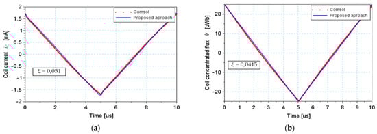
Figure 22.
(a) Inductor current ic waveforms for the case of a rectangular voltage source and a frequency of 100 kHz. (b) Flux linkage Ψ waveform for the case of a rectangular voltage source and a frequency of 1 kHz.
Unfortunately, in Comsol, it is not possible to generate the eddy nor the displacement currents waveforms for a given element; however, the distribution of the currents’ densities are very similar. This allows to state with certainty that the obtained waveforms are reliable.
In Figure 22, Figure 23 and Figure 24, the results for a square wave with a frequency equal to 100 kHz have been shown. Similarly to the previous comparison, the results of both simulation are very similar, which proves the validity of the results presented in the article.

Figure 23.
(a) Distribution of the eddy current density in the ferrite core at time t = 9 us obtained by Comsol Mutliphysics. (b) Distribution of the eddy current density in the ferrite core at time t = 9 us obtained by the proposed approach.

Figure 24.
(a) Distribution of the displacement current density in the ferrite core at time t = 5 us obtained by Comsol Mutliphysics. (b) Distribution of the displacement current density in the ferrite core at time t = 5 us obtained by the proposed approach.
In Table 2, a short comparison between the Comsol simulation and the conducted studies for the square-shaped voltage source has been shown.
Table 2.
The simulations resources’ usage comparison.
According to the Table 2, it can be seen that in the proposed simulation for a similar number of mesh elements and 24-times higher number of time samples, the convergence time was almost 1.5 times higher than in case of Comsol Software. However, the consumption of resources is much lower in the case of the proposed approach. Indeed, the total calculation time is about 30% times lower in case of Comsol software; however, it must be noted that Comsol used all available processor cores, but the proposed approach, due to limited programming resources, used only one core. The simulated rectangular mesh also needs many more resources and is more time consuming, due to the much higher number of nodes. It also needs to be noted that the difference between the number of total time samples of both simulation is overwhelming. It is easy to imagine that when using all available cores for parallel computing and triangular mesh, the total convergence time will be much lower with the proposed approach. The RAM usage is comparable for both simulations. In the proposed approach, the sparse matrixes have been used to reduce the RAM consumption. At a further stage of the work, we plan to start studies on parallelizing the computational process for the elaborated algorithm.
5. Conclusions
To enable the analysis of dielectric current distribution in the considered inductor, we have elaborated an effective tool for analyzing electromagnetic phenomena based on the multi-stage approach to the Finite Element Method. Due to the introduced modification to the formulation A-V-T0, which uses magnetic vector potential A, electric vector potential T0 and electric scalar potential V, we have presented the description of phenomena related to the dielectric displacement current effect. For this purpose, we supplemented the standard reluctance-conductance network model with an additional capacitance network model. Moreover, the application of the Harmonic Balance method and Fixed-Point Method enable the analysis of the ferrite core’s saturation effect.
In this article, we have discussed and explained the fundamental relations and equations that have been used in our calculations. Furthermore, the introduced modifications enabling the time-domain dielectric current distribution analysis have been discussed in detail. Simulations have been run for the system fed by the sinusoidal voltage as well as the rectangular voltage. The output of simulations that are the waveforms of the coil current and coil concentrated flux, as well as the eddy and displacement currents waveforms, have been presented and discussed. To prove the correctness of the obtained results, a simulation has been run, using Comsol Mutliphysics software, for the same object and for the same conditions. The verification showed the convergence of both simulation results. The obtained and verified results have been compared to each other, and the analysis proved that the amplitude of the displacement current is much higher for the rectangular voltage than for the sinusoidal one. The studies show that despite the negligible value of the displacement current amplitude for a low sine source frequency, the discussed current can reach much higher values, especially for square-shaped sources of very-high frequencies.
Author Contributions
Conceptualization, W.L. and R.M.W.; methodology, W.L. and R.M.W.; software, W.L.; formal analysis, R.M.W.; writing—original draft preparation, W.L.; writing—review and editing, R.M.W.; supervision, R.M.W. Both authors have read and agreed to the published version of the manuscript.
Funding
This research received no external funding.
Conflicts of Interest
The authors declare no conflict of interest.
References
- Darwish, M.A.; Trukhanov, A.V.; Senatov, O.S.; Morchenko, A.T.; Saafan, S.A.; Astapovich, K.A.; Trukhanov, S.V.; Trukhanova, E.L.; Pilyushkin, A.A.; Sombra, A.S.B.; et al. Investigation of AC-Measurements of Epoxy/Ferrite Composites. Nanomaterials 2020, 10, 492. [Google Scholar] [CrossRef] [PubMed]
- Jalaiah, K.; Mouli, K.C.; Krishnaiah, R.V.; Babu, K.V.; Rao, P.S.V.S. The Structural, DC Resistivity and Magnetic Properties of Zr and Co Co-Substituted Ni0.5Zn0.5Fe2O4. Heliyon 2019, 5, e01800. [Google Scholar] [CrossRef] [PubMed]
- Hui, S.Y.R.; Zhong, W.; Lee, C.K. A Critical Review of Recent Progress in Mid-Range Wireless Power Transfer. IEEE Trans. Power Electron. 2014, 29, 4500–4511. [Google Scholar] [CrossRef]
- Sanjari Nia, M.S.; Altimania, M.; Shamsi, P.; Ferdowsi, M. Magnetic Field Analysis for HF Transformers with Coaxial Winding Arrangements. In Proceedings of the 2020 IEEE Kansas Power and Energy Conference (KPEC), Manhattan, KS, USA, 13–14 April 2020; pp. 1–5. [Google Scholar]
- Ludowicz, W.; Pietrowski, W.; Wojciechowski, R.M. Analysis of an Operating State of the Innovative Capacitive Power Transmission System with Sliding Receiver Supplied by the Class-E Inverter. Electronics 2020, 9, 841. [Google Scholar] [CrossRef]
- Rivas, J.M.; Han, Y.; Leitermann, O.; Sagneri, A.D.; Perreault, D.J. A High-Frequency Resonant Inverter Topology with Low-Voltage Stress. IEEE Trans. Power Electron. 2008, 23, 1759–1771. [Google Scholar] [CrossRef]
- Regensburger, B.; Kumar, A.; Sinha, S.; Afridi, K. High-Performance 13.56-MHz Large Air-Gap Capacitive Wireless Power Transfer System for Electric Vehicle Charging. In Proceedings of the 2018 IEEE 19th Workshop on Control and Modeling for Power Electronics (COMPEL), Padova, Italy, 25–28 June 2018; pp. 1–4. [Google Scholar]
- Achour, Y.; Starzyński, J. High-Frequency Displacement Current Transformer with Just One Winding. COMPEL 2019, 38, 1141–1153. [Google Scholar] [CrossRef]
- Zhang, X.; Zhao, Y.; Ho, S.L.; Fu, W.N. Analysis of Wireless Power Transfer System Based on 3-D Finite-Element Method Including Displacement Current. IEEE Trans. Magn. 2012, 48, 3692–3695. [Google Scholar] [CrossRef]
- Lu, H.Y.; Zhu, J.G.; Hui, S.R. Experimental Determination of Stray Capacitances in High Frequency Transformers. IEEE Trans. Power Electron. 2003, 18, 1105–1112. [Google Scholar] [CrossRef]
- Grève, Z.D.; Deblecker, O.; Lobry, J. Numerical Modeling of Capacitive Effects in HF Multiwinding Transformers—Part II: Identification Using the Finite-Element Method. IEEE Trans. Magn. 2013, 49, 2021–2024. [Google Scholar] [CrossRef]
- Kanayama, H.; Tagami, D.; Imoto, K.; Sugimoto, S. Finite Element Computation of Magnetic Field Problems with the Displacement Current. J. Comput. Appl. Math. 2003, 159, 77–84. [Google Scholar] [CrossRef][Green Version]
- Koch, S.; Schneider, H.; Weiland, T. A Low-Frequency Approximation to the Maxwell Equations Simultaneously Considering Inductive and Capacitive Phenomena. IEEE Trans. Magn. 2012, 48, 511–514. [Google Scholar] [CrossRef]
- Demenko, A.; Sykulski, J.K. Network Equivalents of Nodal and Edge Elements in Electromagnetics. IEEE Trans. Magn. 2002, 38, 1305–1308. [Google Scholar] [CrossRef]
- Demenko, A. Eddy Current Computation in 3-Dimensional Models for Electrical Machine Applications. In Proceedings of the 2006 12th International Power Electronics and Motion Control Conference, Portoroz, Slovenia, 30 August–1 September 2006; pp. 1931–1936. [Google Scholar]
- Wojciechowski, R.M.; Jedryczka, C.; Szelag, W.; Demenko, A. Description of Multiply Connected Regions with Induced Currents Using T-T0 Method. PIER B 2012, 43, 279–294. [Google Scholar] [CrossRef][Green Version]
- Bíró, O.; Koczka, G.; Preis, K. Finite Element Solution of Nonlinear Eddy Current Problems with Periodic Excitation and Its Industrial Applications. Appl. Numer. Math. 2014, 79, 3–17. [Google Scholar] [CrossRef]
- Lu, J. Harmonic Balance Finite Element Method: Applications in Nonlinear Electromagnetics and Power Systems; John Wiley & Sons: Hoboken, NJ, USA, 2016. [Google Scholar]
- Koczka, G.; Auberhofer, S.; Biro, O.; Preis, K. Optimal Convergence of the Fixed-Point Method for Nonlinear Eddy Current Problems. IEEE Trans. Magn. 2009, 45, 948–951. [Google Scholar] [CrossRef]
- Koczka, G.; Bíró, O. Fixed-point Method for Solving Non Linear Periodic Eddy Current Problems with T, Φ-Φ Formulation. COMPEL 2010, 29, 1444–1452. [Google Scholar] [CrossRef]
- Ausserhofer, S.; Biro, O.; Preis, K. An Efficient Harmonic Balance Method for Nonlinear Eddy-Current Problems. IEEE Trans. Magn. 2007, 43, 1229–1232. [Google Scholar] [CrossRef]
- Kurzawa, M.; Jedryczka, C.; Wojciechowski, R.M. Analysis of Eddy Current System Using Equivalent Multi-Branch Foster Circuit and Edge Element Method. In Proceedings of the 19th International Conference Computational Problems of Electrical Engineering, Banska Stiavnica, Slovakia, 9–12 September 2018; pp. 1–4. [Google Scholar]
- Wojciechowski, R.M.; Jedryczka, C. The Analysis of Stray Losses in Tape Wound Concentrated Windings of the Permanent Magnet Synchronous Motor. COMPEL 2015, 34, 766–777. [Google Scholar] [CrossRef]
- Nowak, L. Field Models of Electromechanical Transducers in Transient States; Publishing House of the Poznań University of Technology: Poznan, Poland, 1999. [Google Scholar]
- Wojciechowski, R.M.; Jędryczka, C. A Description of the Sources of Magnetic Field Using Edge Values of the Current Vector Potential. Arch. Electr. Eng. 2018, 67, 3074–3077. [Google Scholar] [CrossRef]
- Wojciechowski, R.M.; Jędryczka, C. A Comparative Analysis between Classical and Modified Approach of Description of the Electrical Machine Windings by Means of T0 Method. Open Phys. 2017, 15, 918–923. [Google Scholar] [CrossRef][Green Version]
- Demenko, A.; Sykulski, J.K.; Wojciechowski, R. On the Equivalence of Finite Element and Finite Integration Formulations. IEEE Trans. Magn. 2010, 46, 3169–3172. [Google Scholar] [CrossRef]
- Wojciechowski, R.M.; Jedryczka, C.; Demenko, A.; Sykulski, J.K. Strategies for Two-dimensional and Three-dimensional Field Computation in the Design of Permanent Magnet Motors. IET Sci. Meas. Technol. 2015, 9, 224–233. [Google Scholar] [CrossRef]
- Wojciechowski, R.; Demenko, A.; Sykulski, J.K. Calculation of Inducted Currents Using Edge Elements and T–T0 Formulation. IET Sci. Meas. Technol. 2008, 2, 434–439. [Google Scholar] [CrossRef]
- Demenko, A.; Jedryczka, C.; Wojciechowski, R.M.; Sykulski, J.K. Strategies for 2D and 3D Field Computation in the Design of Permanent Magnet Motors. In Proceedings of the 9th IET International Conference on Computation in Electromagnetics (CEM 2014), London, UK, 31 March–1 April 2014; p. 3.09. [Google Scholar]
- Ausserhofer, S.; Biro, O.; Preis, K. A Strategy to Improve the Convergence of the Fixed-Point Method for Nonlinear Eddy Current Problems. IEEE Trans. Magn. 2008, 44, 1282–1285. [Google Scholar] [CrossRef]
Publisher’s Note: MDPI stays neutral with regard to jurisdictional claims in published maps and institutional affiliations. |
© 2021 by the authors. Licensee MDPI, Basel, Switzerland. This article is an open access article distributed under the terms and conditions of the Creative Commons Attribution (CC BY) license (https://creativecommons.org/licenses/by/4.0/).